Essays in theory of the firm and indivisual decision making experiments

Texto completo

(1)Essays in Theory of the Firm and Individual Decision Making Experiments. Giovanni Ursino. TESI DOCTORAL UPF / 2009. DIRECTOR DE LA TESI. Prof. Rosemarie Nagel. (Universitat Pompeu Fabra, Barcelona).

(2) To Giulia. iii.

(3) iv.

(4) Acknowledgments I am grateful to my advisor Rosemarie Nagel for her continued support along the years of my PhD and, more importantly, for having initiated me to the beauty of experiments. I am thankful to Andreru Mas-Colell as well as to Rosemarie Nagel for helping me to spend some time at Harvard. The years in Boston have been an important stage of my professional and personal life. For the great time spent at Harvard I am indebted to Greg Barron, a wonderful coauthor and friend, and to Markus Möbius, who taught me a theorist’s way of thinking. Many discussions with fellow PhD students and Professors alike helped me growing. Just to mention a few, I thank Itay Fainmesser, Paul Niehaus, Bob Gibbons and Oliver Hart at Harvard and MIT, Karl Schlag, Antonio Ciccone, Gino Gancia, Robin Hogarth at UPF. I also want to thank all seminar participants at Harvard, MIT and UPF and in particular Milo Bianchi and Filippo Balestrieri. Marta Aragay and Gemma Burballa have been great helping me with administrative procedures, Marta Araque has been even greater handling my many problems with the bureaucracy while I was abroad and actually tolerating my awful way of being when it comes to administrative issues. As my PhD has been so brutally split in two halves by my visiting period at Harvard, I have been saddened by not having spent enough time with my friends at UPF. Yet they were always present and I felt their enduring friendship while I was away. I would be different had I not met them: Filippo, Davide and Antonio, my first flat mates in the unforgettable Provença apartment, and then Pepe, our permanent guest and Christina, my confrontational friend. The list of UPF friends is long, I stop here but I bear many more in my heart. Boston left me with some good friends as well, Milo and Novita, Filippo, Laura and Davide are the ones I am most attached to. I must also mention my Vespa and Barcelona for the special feeling one gets riding it in this beautiful city. And Boston, for its open skies. My family has been in the background of all this, we have been far apart for many years yet the presence of my parents, my brother and sisters has been constant and fundamental, not only at dismal times. I owe them much, in particular the patience and comprehension for professional choices they shared with me even when they seemed incomprehensible to them. And the joy which welcomed me at each and every trip to Italy: this has been for me pure energy for looking into the future. A special thanks is for Giulia, my everything in the last five years. Nothing would have been the same without her. She has both accompanied me at every time, good and bad, and challenged me on many grounds helping me to become a better person.. v.

(5) vi.

(6) Abstract This thesis is composed of two separate, unrelated chapters. Chapter I, coauthored with Greg Barron, is an experiment in individual decision making. It builds on a small and growing literature which makes the following point: whenever we learn the odds and outcomes of a binary choice problem through experience rather than from a visual description -a prospect- then we take decisions as if we were underweighting rare events. This is in contrast to the well known phenomenon of overweighting rare events in prospect based decisions. Our work contributes to the literature by strengthening this finding in the face of earlier criticism. In particular we find that the underweighting is robust to the elimination of sampling bias which affected previous studies and is absent from ours. We also find that underweighting in choice happens at the same time as overweighting in probability judgment. This remains unexplained. Chapter II introduces a new theory of vertical integration building on the fact that improving a company’s bargaining position is often cited as a chief motivation to vertically integrate with suppliers. In my model firms integrate to gain bargaining power against other suppliers in the production process. The cost of integration is a loss of flexibility in choosing the most suitable suppliers for a particular final product. I show that the firms who make the most specific investments in the production process have the greatest incentive to integrate. The theory provides novel insights to the understanding of numerous stylized facts such as the effect of financial development on the vertical structure of firms, the observed pattern from FDI to outsourcing in international trade, the connection between product cycle and vertical structure, etc.. Resumen Esta tesis se compone de dos partes separadas y sin relación entre ellas. El primer capı́tulo, coautorado con el Profesor Greg Barron, es un experimento en toma de decisiones individuales. Este capı́tulo se construye a partir de una literatura creciente, que enfatiza el siguiente punto: cuando aprendemos las probabilidades y los resultados de una loterı́a a través de la experiencia en vez de la descripción visual del problema -un prospecto- entonces tomamos decisiones como si estuviéramos devaluando eventos poco probables. Esto contrasta con el fenómeno bien conocido de que las probabilidades pequeñas suelen sobrevaluarse cuando se toman decisiones a partir de prospectos. Nuestro trabajo contribuye a la literatura dando fuerza al punto mencionado frente a algunas crı́ticas. En particular, nosotros encontramos que la devaluación sobrevive la eliminación de un problema de muestreo que afectaba trabajos anteriores y está correcto en el nuestro. Encontramos también que hay devaluación de probabilidades pequeñas vii.

(7) en toma de decisiones al mismo tiempo que sobrevaluación en juicio sobre las mismas probabilidades. Este último resultado no puede ser explicado. El segundo capı́tulo introduce una nueva teorı́a de integración vertical a partir del hecho de que aumentar el poder contractual de una empresa es citado muy a menudo como una razón para integrarse verticalmente con los proveedores. En mi modelo las empresas se integran para ganar poder contractual hacia proveedores no integrados en la cadena productiva. El coste de la integración es una pérdida de flexibilidad a la hora de escoger los proveedores más apropiados para un particular producto final. Muestro como las empresas que tienen inversiones más especı́ficas en el proceso productivo tienen un mayor incentivo a integrarse. La teorı́a presentada permite explicar numerosos hechos estilizados como el efecto del desarrollo financiero sobre la estructura vertical de las empresas, la evolución que se observa de inversión extranjera directa a outsourcing en el comercio internacional, la conexión entre ciclo de vida del producto y la estructura vertical, etc.. viii.

(8) Foreword This thesis is composed of two separated and unrelated chapters. The reason why there is not a common ground behind these two works is that, along the course of my PhD, I have developed an interest for different topics. I have then cultivated such different interests up to the point of producing an original piece of work in both fields. The ordering is chronological. The bibliography is by chapter to avoid confusion. The introductions to each chapter dig deeper into each field, yet I shall briefly introduce each peace of work here. Chapter 1 is a work in the field of individual decision making. It belongs to a small and growing literature which originates by Ido Erev and his collaborators (Erev and Barron (2005)) and has an ambitious program: it challenges the validity of Prospect Theory whenever decisions are taken from experience. This is because, when learning happens through experience as opposed to description, then it is observed that small probabilities are underweighted rather than overweighted. The proposed alternative model are learning models such as reinforcement learning, etc. Given the wide use of Prospect Theory as a normative theory of individual decision making and, most importantly, the pervasiveness in daily life of experience based decisions, the research program of which Chapter 1 is a piece is a very relevant one. Chapter 2 belongs to the organizational economics literature and in particular it adds to the theory of the firm as first developed by Coase (1937) and later by Williamson (1985), Williamson (2002), Grossman and Hart (1986) and Hart and Moore (1990). The field is vast and many theories have been proposed. Yet, while a dominant paradigm has emerged, the Property Rights approach, there is not a comprehensive theory of the boundaries of the firm, i.e. of vertical integration. Chapter 2 contributes to the building of such a theory by incorporating an aspect of vertical integration which has not been formally modeled yet: the fact that oftentimes firms vertically integrate in order to gain bargaining power with respect to non integrated suppliers. Motivated by this observation Chapter 2 uses elements of both the Property Rights and the Transaction Cost Economics approaches to construct a new theory of vertical integration.. ix.

(9) x.

(10) Contents Abstract . . . . . . . . . . . . . . . . . . . . . . . . . . . . . . . . . . . . . .. vii. Foreword. ix. . . . . . . . . . . . . . . . . . . . . . . . . . . . . . . . . . . . . .. 1 Underweighting Rare Events in Experience Based Decisions: Beyond Sample Error. 3. 1.1. Introduction . . . . . . . . . . . . . . . . . . . . . . . . . . . . . . . . .. 3. 1.2. Experiment 1: decisions under risk using a sampling paradigm . . . . .. 4. a.. Method . . . . . . . . . . . . . . . . . . . . . . . . . . . . . . .. 4. b.. Results . . . . . . . . . . . . . . . . . . . . . . . . . . . . . . . .. 6. Repeated choice vs. free sampling . . . . . . . . . . . . . . . . . . . . .. 7. a.. Revisiting the Barron and Erev (2003) data . . . . . . . . . . .. 8. b.. Experiment 2: repeated choice and judgment . . . . . . . . . . .. 9. Discussion . . . . . . . . . . . . . . . . . . . . . . . . . . . . . . . . . .. 11. 1.3. 1.4. 2 Supply Chain Control:A Theory of Vertical Integration. 13. 2.1. Introduction . . . . . . . . . . . . . . . . . . . . . . . . . . . . . . . . .. 13. 2.2. Theory . . . . . . . . . . . . . . . . . . . . . . . . . . . . . . . . . . . .. 15. a.. Model Setup . . . . . . . . . . . . . . . . . . . . . . . . . . . . .. 15. b.. Discussion . . . . . . . . . . . . . . . . . . . . . . . . . . . . . .. 18. c.. Analysis . . . . . . . . . . . . . . . . . . . . . . . . . . . . . . .. 18. 2.3. Endogenous Investment . . . . . . . . . . . . . . . . . . . . . . . . . . .. 24. 2.4. Applications and predictions of the model . . . . . . . . . . . . . . . .. 25. 2.5. Conclusion . . . . . . . . . . . . . . . . . . . . . . . . . . . . . . . . . .. 29. References to Chapter 1. 31. References to Chapter 2. 33. A Appendix to Chapter 2. 37. 1.

(11) 2.

(12) 1. 1.1. Underweighting Rare Events in Experience Based Decisions: Beyond Sample Error Introduction. Several recent papers have focused on the description-experience gap, the observation that while people tend to overweight small probabilities in decisions from description, they appear to underweight small probabilities in decisions from experience. Fox and Hadar (2006) (hereafter FH) note that, in Hertwig et al. (2004) (hereafter HBWE), behavior that appears to reflect underweighting can be explained by statistical sampling error; it follows from the binomial distribution that people are more likely to undersample rare events then to over-sample them. FH demonstrate that the two-stage choice model (Fox and Tversky (1998)) that assumes that choice can be predicted from estimated probabilities can account for HBWE’s finding when observed frequencies are substituted for the underlying probabilities. This paper’s main goal is to examine the usefulness of FH’s account in explaining underweighting of rare events beyond the HBWE paradigm. As FH point out, while decisions from description are decisions under risk (as the lotteries are known) decisions from experience are often decisions under uncertainty when the lotteries are represented as unlabeled buttons. Underweighting of rare events has been observed in two different paradigms under uncertainty. In the first, Repeated Decision Making (as in Barron and Erev (2003); Erev and Barron (2005)), people repeatedly choose between two unmarked buttons, each representing a static lottery. After each choice one outcome is drawn from the chosen distribution and is added or subtracted from the subject earnings. In the second paradigm, Free Sampling (as in HBWE), two unmarked buttons again represent static lotteries. However, subjects only make a single choice between the two options. Before they choose, subjects are allowed to sample outcomes from the two buttons as often as they wish without incurring actual gains or losses. Once satisfied with their search, subjects make a single choice and one outcome is drawn from that button’s associated distribution. These two paradigms, while different from each other, have in common the incremental acquisition of information over time about the underlying lotteries. Additionally, both paradigms demonstrate decision making under knightian uncertainty. They do not constitute decisions under risk since, no matter how many outcomes are sampled, there will be heterogeneous beliefs about the underlying distributions that remain unknown (Fox and Hadar (2006)). This paper contributes to the existing literature on the description-experience gap in two main ways: as the underweighting of rare events has been observed in both the repeated choice paradigm and the free sampling paradigm we examine the role of statistical sampling error in both contexts. First, in Experiment 1 we introduce a version of the sampling paradigm that specifically examines decisions under risk, where the underlying 3.

(13) choice distributions become known through the sampling process. This paradigm allows us to examine not only the predictions of the two-stage model, but also those of Prospect Theory since the decisions are made under risk. Secondly, we turn to the repeated choice paradigm through a re-examination of the repeated choice data from Barron and Erev (2003) while controlling for sample error. Finally, in Experiment 2 we examine a repeated choice task designed to be free of sampling error. The results of the two experiments and the new analysis of past data all demonstrate the underweighting of rare events in decisions from experience, i.e., the description-experience gap, even in the absence of statistical sample error. These results suggest that sample error, while being sufficient for the observed underweighting in HBWE, is not necessary for underweighting to occur in decisions form experience. The results remain consistent with Hertwig et al. (2004) ’s explanation; that underweighting is due to over reliance on small samples drawn from memory (Kareev (2000); Barron and Erev (2003); Erev and Barron (2005); Hertwig et al. (2004)).. 1.2. Experiment 1: decisions under risk using a sampling paradigm. Sampling error plays a role in the “sampling paradigm” due to the paradigm’s uncertain nature. No matter how many outcomes are sampled, beliefs will remain heterogeneous as to the underlying distribution. One way to control for this, that we explore here, is to employ sampling without return from a finite population. In other words, the decision maker gets to see all the outcomes one at a time. Once the entire population of outcomes has been sampled the decision maker has full information about the prospects’ outcomes and their likelihoods. Any choice based on this information (about drawing a single outcome form two such populations) will be a decision under risk. If the descriptionexperience gap is indeed driven by sample error, it should not be observed when the entire population has been exhaustively sampled. Alternatively, if the over reliance on small samples drawn from memory plays a significant role in decisions from experience, a gap should still be observed.. a.. Method. One hundred twenty one students of the Boston area served as paid volunteers in the experiment. Students were at the undergraduate or graduate school level and came from local universities (Harvard, Boston University and Boston College). During each session participants went through two conditions “10%” and “20%”, that were identical with the exception of the risky lottery. The order of the two conditions was randomized. Each condition consisted of two phases. In the first phase, described 4.

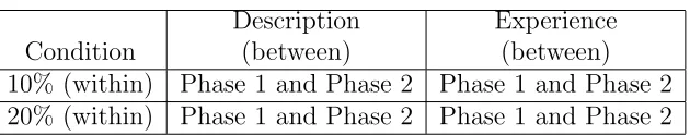
(14) below, we identified a pair of lotteries for which the participant was indifferent and in the second phase the participant made a single choice between the lotteries. The choice was made either from Description or from Experience (our two between-subjects conditions). Table 1.1 shows the overall design of the experiment. Participants were paid according to one of the four phases they went through, randomly chosen at the end of the experiment. Participants also received a $10 show up fee and the average total payment was $27.20. Table 1.1: Design of Experiment 1 Condition 10% (within) 20% (within). Description (between) Phase 1 and Phase 2 Phase 1 and Phase 2. Experience (between) Phase 1 and Phase 2 Phase 1 and Phase 2. Phase 1 was a BDM-like procedure (Becker et al. (1964)) meant to elicit the value, X, for which participants were indifferent between the relatively safe (S) and risky (R) lotteries below: ∙ S:($X, 0.9; 0) or R:($40, 0.1; 0) in Condition 10% ∙ S:($X, 0.8; 0) or R:($20, 0.2; 0) in Condition 20% The probabilities of 0.1 and 0.2 were chosen keeping with the values for which over and underweighting are typically observed in decisions from description and from experience. To arrive at the point of indifference, X indiff, each participant sequentially chose between pairs of lotteries, as above, with alternative values for X. X randomly started out at either 0 or 40 (0 and 20 for Experiment B) and then increased by half the range if R was preferred and decreased by half the range otherwise. After the thirteenth choice we were able to identify the implied indifference point for each subject. Participants were told that their Phase 1 payoff would be an outcome drawn from their preferred lottery in a randomly selected pair, chosen from the 13 pairs they were presented with. The outcome was not shown until the end of entire session. We employed this procedure in an effort to control for heterogeneity in preferences for risk. Thus, any difference in choices in the next phase can only be traced to the difference in the two conditions in Phase 2 and will not be influenced by pre-existing preferences over particular lotteries. In Phase 2 of each experiment participants were randomly allocated between a Description and an Experience condition, between subjects, and made an actual decision between ($X indiff -$0.02, 0.9) and R:($40, 0.1) (or ($X indiff -$0.02, 0.8) and R:($20, 0.2) for condition 20%). We subtracted 2 cents from X indiff to avoid participants feeling committed to their previously indicated indifference point. We did not expect such a small amount to have a large effect on the choices in Phase 2 although it arguably induces a preference for the risky lottery. 5.

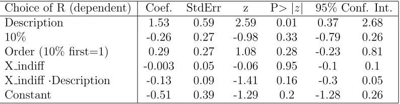
(15) Participants in the Description condition made a single choice between the two prospects that were described as in the previous paragraph. In the Experience condition participants were not shown the lotteries. Instead, they were presented with two unmarked buttons and were told that they corresponded to two boxes containing 100 balls each. Each ball was marked with one of only two possible outcomes for each box. They were then instructed to sample from each box (by clicking on the two buttons in any order they desired) all the balls and to observe their values, one by one until both boxes were empty. The boxes would then be refilled with the same balls and they would choose a box from which to draw a single ball for real money. They were provided with paper and pencil and could keep a tally throughout the experiment if they wished. After sampling all the outcomes subjects made a single choice based on their experience of the two distributions. Subjects did not receive feedback on the outcome until the end of the entire session. After both Phase 1 and 2 were completed, the procedure was repeated for the experiment not yet completed (10% or 20%). When all data collection had been completed subjects were shown their outcomes for Phases 1 and 2 of experiments A and B. Each outcome was a draw from the participants selected lottery for that phase (randomly selected among the thirteen pairs of the BDM procedure for Phase 1). One of these four outcomes was randomly chosen for the participants’ payoff. This rule allowed us to make the BDM procedure incentive compatible while keeping the experiment financially affordable.. b.. Results. Table 1.2 shows the mean choice of the risky lottery R in all 4 conditions. Aggregating over both 10% and 20%, the proportion of Risky choices in the Experience condition (38%) was significantly lower than in the Description condition (56%) (𝛽 = 1.53, z=2.59, p<0.01, first row in logistic regression of Table 1.3). There was no significant difference between conditions 10% and 20% nor was there an effect of the order the conditions were presented or of the indifference point selected by the participant (rows 2-4 of Table 1.3, all non significant). This result is consistent with the description-experience gap and implies underweighting of the rare event in a decision under risk and in the absence of sampling error. Table 1.2: Mean Choice of R Condition 10% 20%. Description 0.52 0.59. Experience 0.35 0.4. Table 1.4 reports the proportion of choices correctly predicted by Prospect Theory in all the conditions. The prediction was calculated per each subject using the parameters 6.

(16) Table 1.3: Logistic Regression Choice of R (dependent) Coef. Description 1.53 10% -0.26 Order (10% first=1) 0.29 X indiff -0.003 X indiff ⋅Description -0.13 Constant -0.51. StdErr 0.59 0.27 0.27 0.05 0.09 0.39. z 2.59 -0.98 1.08 -0.06 -1.41 -1.29. P> ∣𝑧∣ 0.01 0.33 0.28 0.95 0.16 0.2. 95% Conf. Int. 0.37 2.68 -0.79 0.26 -0.23 0.81 -0.1 0.1 -0.3 0.05 -1.28 0.26. estimated in Tversky and Kahneman (1992) and the (modified) X indiff taken from the BDM procedure of Phase 1. The prediction was then compared to that subject’s behavior. As can be seen in the table, Prospect Theory is significantly more useful in predicting the decisions from description than those from experience even though both decisions were decisions made under risk. Table 1.4: Proportion predicted by PT Condition 10% 20%. 1.3. Description 0.62 0.61. Experience 0.38 0.42. Repeated choice vs. free sampling. Less clear is the role of sampling error in the repeated choice paradigm. The paradigm is arguably quite prevalent in real life settings where we learn from the outcomes of our previous choices and most learning models have been developed with the explicit goal of understanding this process. While sampling per se is not an issue in this paradigm, since outcomes are incurred and not merely sampled, the statistical phenomenon of sampling error and its effect on decision making remain an issue. Simple learning models of repeated choice predict that underweighting of rare events will occur due to an over reliance on small samples (Barron and Erev (2003); Erev and Barron (2005)) and/or due to the “hot stove” effect (Denrell and March (2001)) where a bad outcome decreases choice from the same distribution again in the future. In both cases, while the models predict that sample error can increase the apparent underweighting of rare events, they also predict that underweighting will persist even in the absence of sampling error. These predictions stand in contrast to the account of underweighting given by FH in which underweighting should disappear when sample error is controlled for. The remainder of this paper examines this hypothesis in both 7.

(17) a reanalysis of the Barron and Erev (2003) repeated choice data and a laboratory experiment.. a.. Revisiting the Barron and Erev (2003) data. If sample error is the prime mechanism driving the gap between experience and description based decisions, the gap should disappear when we examine subjects who observed the rare event approximately the expected number of times. To evaluate this assertion we identified the 6 problems studied by Barron and Erev (2003) for which the analysis is relatively straight forward. The 6 lottery pairs, and their problem number from the Barron and Erev (2003) paper, appear in Table 1.5. Each pair includes one risky two-outcomes lottery and one safe certain-outcome lottery. The lottery with the higher expected value (H) appears in second column and the lottery with the lower expected value (L) appears in the third column. The fourth column shows the proportion of H choices aggregated over subjects and over 400 trials. As noted in Barron and Erev (2003), behavior in each of the problems is consistent with underweighting of the rare event and is inconsistent with Prospect Theory (assuming the parameters estimated in Tversky and Kahneman (1992)). To examine the behavior of those subjects whose observed sample of outcomes was relatively unbiased we first computed, for each individual, the observed frequency of the rare event in the risky lottery. We then removed all subjects whose observed frequency of the rare event was greater or less then one standard deviation from the expected frequency. The remaining number of subjects appears in the right most column of Table 1.5. Table 1.5: Barron and Erev (2003) decision problems. Problem H 4 4, .8 6 -3 7 10, .9 8 -10, .9 9 32, .1 11 -3 * p<0.05. Proportion of H choices B&E +/- 1std. N P(H) P(H) (from 24) L 3 0.63 0.64 10 -4, .8 0.6 0.56 15 9 0.56 0.63 20 -9 0.37 0.47* 17 3 0.27 0.43* 11 -32, .1 0.4 0.33 11. As shown in column 5 of the table, in 4 of the 6 problems the proportion of H choices in the restricted data set did not change significantly. In two of the 6 problems, 8 and 9, the less biased subjects chose H significantly more often. However, even in these two 8.

(18) problems the choice of the modal subject was the same as that in the unrestricted data set (i.e., they continued to choose L most of the time). In summary, the reanalysis of the repeated choice paradigm in Barron and Erev (2003) does not support FH’s argument that what appears to be underweighting of rare events is in fact primarily the result of sample error. Even when observed outcomes approximate expected distributions, behavior remains consistent with the underweighting of small probabilities. Three shortcomings of the above analysis need to be addressed. First, the analysis performed was not particularly sensitive. Observed frequencies of the rare event still fluctuated in the +1/-1STD range for individual subjects, each of whom was incurring a different stream of payoffs from choosing safe and risky options. Secondly, the stream of observed payoffs was path dependent since subjects only observed the outcome from the chosen option (i.e., forgone payoffs were not observed). Underweighting in this case can be the result of the ”hot stove effect” which effectually leads to a biased sample as people cease to choose an option after an unlucky streak of bad outcomes. Thirdly, subjects were not asked to estimate the probability of the rare event. Thus, we still don’t know if any judgment error has occurred and can not directly test the predictions of the two-stage choice model that uses estimations to predict choice. We address all these limitations in an experiment using the repeated choice paradigm where all subjects observe the same stream of incurred and forgone payoffs. Additionally, the complete stream of payoffs is representative of the underlying payoff distributions and we elicit probability judgments of the rare event.. b.. Experiment 2: repeated choice and judgment. Method Twenty-four Technion students served as paid participants in the study and performed both a binary choice task and a probability assessment task. The binary choice task was performed under uncertainty one hundred times (with immediate feedback on both obtained and forgone payoffs) with the probability assessment task following each choice in rounds 51-100. Upon completion, participants performed a one-time retrospective probability assessment task. In the binary choice task, participants chose between two unmarked buttons presented on the screen. Each button was associated with one of two distributions referred to here as S (for safe) and R (for risky). The S distribution provided a certain loss of 3 points while the R distribution provided a loss of 20 points with probability 0.15 and zero otherwise. Thus, the two distributions had equal expected value and the exchange rate was 100pts = 1 Shekels (about 29 US cents). 9.

(19) To assure that all subjects experienced the same representative sequence of outcomes we first produced random sequences of 100 outcomes and the first sequence with an observed probability of 0.15 for the -20 outcome was used for all participants. The sequence provided the -20 outcome on rounds 12, 15, 19, 20, 21, 23, 25, 35, 40, 41, 60, 73, 80, 87, and 96. In the probability assessment task, performed after each binary choice in trials 51-100, participants were prompted to estimate the chances (in terms of a percentage between 0 and 100) of -20 appearing (on the R button) on the next round. After completing 100 rounds participants were asked to estimate (“end-of-game estimates”), to the best of their recollection, two conditional subjective probabilities (SP): (1) the chances of -20 appearing after a previous round with a -20 outcome [SP(-20∣20)] and (2) the chances of -20 appearing after a previous round with a 0 outcome [SP(-20∣0)]. Results The mean probability assessment from trials 51-100, aggregated over trials and over subjects, was 0.27. This value is significantly larger than 0.163, the mean running average of the observed probability of the -20 outcome (t[23] = 3.11, p <.01). Thus, the results reflect overestimation of the rare event. As shown in Table 1.6, participants’ aggregate proportion of R choices was 0.74 (significantly larger than 0.5, t[23] = 7.47, p <.001). This result is consistent with the assertion of underweighting of rare events in choice. The rate of R choice over trials 51-100 was 0.80 (significantly larger than 0.5, t[23] = 6.78, p <.001). Table 1.6: A summary of the aggregate results of Experiment 2 Statistic Trials 1-100 Trials 51-100 P(R) proportion of R choices 0.74 (0.5*)† 0.8 (0.5*)† SP(-20) Mean subjective assessment of the probability − 0.27 (0.16*)† of a -20 outcome *p<0.01 † The numbers in parenthesis denote the null hypotheses for the test reported in the text. All t-tests are one-sample tests unless otherwise noted. Comparison of the judgment and the choice data for trials 51-100 is inconsistent with FH’s account for underweighting. While subjects’ choices are consistent with underweighting the rare event, they consistently overweighted the rare event in their probability estimations. While the objective probability of the rare event was 0.15 and its 10.

(20) mean observed proportion (recalculated after each trial) was 0.16, subjects mean estimation was 0.27 reflecting significant overweighting. This pattern cannot be predicted by the two stage choice model that applies Cumulative Prospect Theories weighting function1 . Applying that function, which assumes overweighting of small probabilities, to the objective, the observed or the estimated probabilities leads to a prediction of overweighting in choice, and not underweighting as was observed. In order to confirm that the different reactions occur at the level of individual subjects a pair-wise within-subjects analysis was performed. For 63% (15/24) of the participants, assessment and choice results were not consistent in terms of the implied weighting of the -20 outcome. Overestimation and underweighting of rare events was found to occur in 100% of these 15 cases.. 1.4. Discussion. We examine FH’s assertion that decisions reflecting the underweighting of rare events may be the result of statistical sample error. As HBWE point out, rare events are more likely to be under sampled than oversampled due to skewness of the binomial distribution. To see if sample error is a necessary condition for underweighting to occur, we present two experiments and one re-analysis of past data that control for, or eliminate the possibility of sample error. In all three data sets behavior continued to be consistent with the underweighting of rare events in decisions form experience. This paper’s first contribution is in showing that while sample error may be sufficient for implied underweighting to occur, it is clearly not a necessary condition. The findings shed some light on the distinction between decisions form experience and from description. It is tempting to classify the former as a decision under uncertainty and the latter as a decision under risk. However, in Experiment 1 we examine a hybrid paradigm where a decision from experience is taken under risk as all the outcomes and their frequencies were known by the decision maker. The significant descriptionexperience gap that was observed is inconsistent with models that assume overweighting of rare events under risk (i.e., Prospect Theory). One remaining possibility is that people are making a judgment error, even if the sample is unbiased, and are underestimating the rare event. Experiment 2 examined this possibility by eliciting probability estimates throughout the experiment. While there was indeed a judgment error, it was in the opposite direction. People were overestimating the rare event while their choices (within subject) reflected underweighting. Again, 1. There are parameters for which Prospect Theory’s weighting function will imply underweighting of rare events. However, such parameterization is a contradiction to the fourfold pattern of risk attitudes observed in decisions form description. It is this pattern that the model was offered to elegantly quantify in the first place.. 11.

(21) this pattern of results cannot be predicted by models that assume Prospect Theory’s weighting function such as the Two-stage choice model (Fox and Tversky (1998)). Overweighting of estimations (e.g., Viscusi (1992); Erev et al. (1994)) and underweighting in choice have both been demonstrated in other research, but never concurrently and within subject. Decisions from experience remain qualitatively different than decisions from description in ways beyond subjects’ tendency to under sample lotteries, as was the case in Hertwig et al. (2004) sampling paradigm. All the data presented in the current paper are consistent with the assumption that decisions from experience rely on small samples drawn from memory and can be described by simple learning and sampling models that quantify this assumption.. 12.

(22) 2. Supply Chain Control:A Theory of Vertical Integration. 2.1. Introduction. I consider how vertical integration affects the bargaining power of the integrating firms against non-integrated firms in the supply chain. Integration has costs because it limits an assembler’s flexibility in choosing the most suitable suppliers for a particular end product. However, by gaining bargaining power the assembler can appropriate a larger share of the total revenue which can make integration a profitable strategy for the assembler. I use two examples from the PC and the cell phone industry to motivate my analysis. In the PC industry, IBM and Apple Inc. followed very different strategies. IBM only controlled the hardware of the original PC and had Microsoft provide the operating system. In contrast, Apple controlled both the operating system and the hardware of the Macintosh PC from the start. Within a few short years, Microsoft became the dominant player in the PC industry and in 2005 IBM exited the PC business by selling its remaining factories. Apple, on the other hand, was able to keep its PC business highly profitable and thriving. Apple’s decision did not come without costs because the company was often slow in updating its operating system.1 Ultimately, however, Apple’s decision to integrate software and hardware and sacrifice flexibility proved profitable. In the cell phone industry, there has been substantial disagreement about the optimal level of vertical integration and the boundary between in-house and outside procurement has shifted a number of times during the past 15 years. In the 1990s, large handset manufacturers such as Motorola, Nokia and Ericsson outsourced a lot of the design and software development to suppliers in Taiwan, Singapore and India. These suppliers gained crucial knowledge and expertise as a result which allowed some of them to become fierce competitors on their own right.2 The business press has acknowledged the importance of vertical integration for bargaining with suppliers. For example, the Financial Times stated in a special report on vertical integration that “Another reason to integrate vertically is to affect bargaining power with suppliers” (November 29, 1999). In my model, each final product requires a continuum of inputs which are each produced by a specialized supplier. Inputs in my model are complements and each supplier has ex1. For example, Windows 95 was considered a more stable system than the Apple OS 7. In fact, the main reason behind IBM’s decision not to develop the operating system in-house was a desire to bring the PC to market as quickly as possible. 2 For example, HTC now produces own brand smart phones as well as those of its clients. The same is true for Compal and the goal of Flextronics’ CEO Michael E. Marks -as reported by Business Week (March 21, 2005)- is to make Flextronics a low-cost, soup-to-nuts developer of consumer-electronics and tech gear.. 13.

(23) ante equal ability to hold up assembly of the final product. I assume that inputs differ in their specificity, defined by the extent to which the revenue produced by each supplier is subject to hold up. The assembler of the final product has the opportunity to purchase suppliers and integrate them into a single company. The integrated company obtains bargaining power that is disproportionately larger than the share of the production process that is being integrated in the single company. In return, the assembler loses the ability to choose the most suitable companies for production of the final product. As long as the inefficiency that is caused by integration is not too severe a well defined integrated equilibrium exists. I show that the vertically integrated company will incorporate those suppliers who are required to make the most specific investments. The intuition behind this result is that those suppliers are most vulnerable to hold-up and therefore benefit the most from an increase in bargaining power. In my basic model, integration always has negative welfare consequences because integration affects the distribution of revenue between integrated and non-integrated firms but actually decreases total available revenue (due to the decrease in flexibility). In an extension of the model I allow firms to vary the level of investment. I show that, under certain conditions, integration can improve welfare because firms with specific investments will invest more after integration since their investments are better shielded from expropriation. My model predicts that a greater incidence of incremental innovation, the increased human to physical capital ratio and the rise of modern financial markets (Rajan and Zingales (2001); Acemoglu et al. (2005)) lead to less vertical integration which is consistent with recent trends in developed economies. On the other hand, I also show that industries with a high level of basic research give rise to vertically integrated firms (see Acemoglu et al. (2004)). The prediction that the vertically integrated company incorporates those suppliers who are required to make the most specific investments explains why Japanese auto makers have historically been unwilling to import US auto parts with high technological content (Spencer and Qiu (2001); Qiu and Spencer (2002)). My model also helps to explain why vertically integrated firms are mostly found in developed countries while developing countries host predominantly small-sized firms. Using a similar approach as in Antràs (2005) my model can also explain the recent shift from FDI to outsourcing in international trade (see also Vernon (1966)). My work shares several characteristics with the Property Rights theory of the firm as developed in Grossman and Hart (1986) and Hart and Moore (1990). Just as in the property-rights view firms’ investments can be appropriated by a partner. However, my model analyzes the bargaining power of integrated (inside) firms versus non-integrated (outside) firms. My model also contributes to our understanding of the optimal boundary of the firm. This question was famously posed by Coase (1937) and became the cornerstone of Transaction Cost Economics (Williamson (1985), Williamson (2002)). Although my model resembles models found in the literature on vertical foreclosure (Salinger (1988), Hart and Tirole (1990), Kranton and Minehart (2002)) the mecha14.

(24) nism is quite different. In the foreclosure literature different assemblers produce an homogeneous final good and compete with each other - integration serves as a means to exclude the competing assembler from access to crucial supplier. In contrast, each assembler in my model is a monopolist in the final product market. Finally, my model shares some features of Acemoglu et al. (2007), most notably the way contractual incompleteness is modeled -more on this later. In the next section I introduce and analyze the basic model. Section 2.3 endogenizes the investment decision of firms. In section 2.4 I apply the model to explain a series of stylized facts. Section 2.5 concludes.. 2.2. Theory. This section introduces a simple model that exhibits the tradeoff between the bargaining advantage that vertical integration provides and the loss in flexibility.. a.. Model Setup. I model an industry that produces 𝐿 variants of a final product (such as the automobile industry or the cell phone industry). Each final product variant is assembled from a set of individual essential components3 which I index by 𝑖 ∈ [0, 1]. Each type 𝑖 component is produced by a type 𝑖 firm. Since there are different variants there are also multiple firms of each type, one per variant. Components are put together by an assembler there is one assembler for each final product variant. Each component can be either “perfect” or imperfect for the final product. The share of perfect components in a product, 𝑥, determines the value of the final product variant in the market. For the sake of simplicity I assume a simple linear specification and define the final revenue, 𝑆, as: 𝑆 = 𝜋𝑥 (2.1) In order to produce each firm has to make an investment of 1. Therefore, total profits for a final product variant with a share 𝑥 of perfect components are 𝜋𝑥 − 1. Firms differ in their ability to appropriate the available revenue 𝑆. I assume that each firm type 𝑖 can appropriate a revenue of 𝑟(𝑖)𝑆 by investing where 𝑟(𝑖) is an increasing ∫1 function that lies between 0 and 1. The remaining revenue 𝑆˜ = 0 [1 − 𝑟(𝑖)] 𝑆 is subject to negotiation between firms which I describe in greater detail below. The function 𝑟(𝑖) is the specificity function and captures the extent to which a firm’s claim to the revenue is subject to negotiation between firms. For example, the revenue of a firm 3. A final product cannot be produced and/or sold without each and every component, hence components are essential. In other words, the production function is Leontief.. 15.

(25) with specificity 𝑟(𝑖) = 0 fully depends on its ability to negotiate with other component suppliers. On the other hand, a firm with specificity 𝑟(𝑖) = 1 does not have to rely on negotiation at all. I consider the specificity function as determined by production technology4 . In section 2.4 I analyze how vertical integration decisions differ across industries with different specificity functions. Figure 2.1: Timing for vertical integration game and negotiation over revenue Assemblers buy subset of suppliers Stage 1. Firms align with assemblers Stage 2. -. Firms make investments Stage 3. -. Revenue is divided Stage 4. The remainder of the model describes precisely how firms divide the appropriable revenue 𝑆˜ among themselves and how they can affect the distribution of revenue through vertical integration. Figure 2.1 lists the four main stages of the model. Stage 1: Vertical Integration Game In the first period each assembler can buy a subset 𝐼 ⊂ [0, 1] of component firms and form a vertically integrated firm. To simplify notation I will focus on the cases where assemblers use symmetric strategies such that each assembler buys the same portfolio of firms. I will later show that the assemblers will prefer to buy a contiguous set of ∫ firms 𝐼 = [0, 𝑁 ] where 0 ≤ 𝑁 ≤ 1 and 𝑁 = 𝐼 𝑑𝑖. However, the model does not restrict assemblers to such strategies In equilibrium the assembler has to offer each firm the profit the firm would derive from remaining non-integrated. Stage 2: Alignment Stage In the second period non-integrated firms choose assemblers. I assume that each nonintegrated firm of type 𝑖 produces a “perfect” component for exactly one final product variant. For all other variants the firm’s component is non-perfect. This gives rise to a simple assignment of non-integrated firms to assemblers: each type 𝑖 firm will choose its optimal variant. 4. Modeling investment specificity without reference to the existence of a second best -outside optionmarket is not novel. For instance Acemoglu et al. (2007) model contractual incompleteness by allowing suppliers’ activities to be only partially verifiable: the degree of verifiability of a supplier’s activities is a primitive in their model and determines her bargaining outcome. Moreover, a large literature dating back at least to Macaulay (1963) attests that, when writing breach of contract provisions, businessmen don’t actually believe they have a way out the contract other than the payment of damage fees. In other words, when dealing with complex transactions, managers normally don’t take it seriously the existence of an outside market to sell their specific components in case the original contract is breached; rather, in such cases they relay on the payment of damage fees at best.. 16.

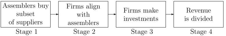
(26) I assume that each component produced by an integrated firm is perfect with probability 𝛾 ≤ 1. The parameter 𝛾 is determined by technology and captures the loss of flexibility that vertical integration entails. The lower 𝛾 the more costly is vertical integration. Integration by itself therefore induces a welfare loss because it bounds a portfolio of component suppliers together before uncertainty about a supplier’s suitability for a particular final product variant is resolved. For example, a vertically integrated car manufacturer might discover that it needs to increase the share of fuel efficient cars in its lineup. However, because the company is integrated it might be forced to make use of gas-guzzling internally produced engines rather than source engines from suppliers of fuel-efficient engines5 . Stage 3: Investment Stage In this stage all firms decide whether to invest one unit of capital. Production of a final product variant is Leontief - therefore it cannot take place unless all suppliers make the required investment. Stage 4: Bargaining Stage In the bargaining stage both integrated and non-integrated firms divide the appropriable ˜ revenue 𝑆: ∫ 1 ˜ [1 − 𝑟(𝑖)] 𝑑𝑖 (2.2) 𝑆 = 𝜋(1 − 𝑁 + 𝑁 𝛾) 0. I assume that firms engage in Nash bargaining6 . One problem with Nash bargaining in the presence of a vertically integrated firm is that integration tends to reduce bargaining power. To see the problem, consider simple bargaining over a pie of size 1 with three firms with equal bargaining power and outside option 0. Each firm will receive 31 of the pie. Now assume that two firms integrate and bargain as a single entity with the third firm. Now the integrated firm will receive 21 of the pie - therefore integration hurts a firm’s bargaining power. I follow Kalai (1977) and assume that the integrated firm has Nash weight 𝑁 7 . This implies that integration per se does neither decrease nor increase a firm’s bargaining power. Instead, in my model the division of the pie will be affected by the outside option of integrated and non-integrated firms. 5. Of course an assembler might well procure both internally and from outside at the same time, possibly at a higher cost. Here I focus on a more drastic in or out decision. 6 Another widely used concept is the Shapley Value. I use Nash Bargaining because a) being a non cooperative solution concept it fits better the zero-sum opportunistic nature of the game studied here; and b) given the Leontief production function, the marginal contribution of each supplier in Shapley Value would be equal to the whole value of production and the resulting share would be trivially equal across suppliers. 7 Kalai (1977) deals with group aggregation of players in multi-players Nash bargaining problems and, loosely speaking, suggests that a group be weighted by the number of its components. This implies that a group-player enjoys a share of the pie proportional to its size.. 17.

(27) I assume that a non-integrated firm has outside option 08 . The integrated firm, however, can replace any non-integrated firm with a fringe supplier. Fringe suppliers always produce imperfect components9 . Therefore, if bargaining in the last period breaks down the integrated firm will bargain with fringe suppliers in an auxiliary bargaining round where the appropriable revenue is now10 : 𝑆ãux = 𝜋𝑁 𝛾. ∫. 1. [1 − 𝑟(𝑖)] 𝑑𝑖. (2.3). 0. In this auxiliary round the outside option of both integrated firm and fringe suppliers is zero.. b.. Discussion. Intuitively, in my model vertical integration improves the bargaining power of integrating firms in the bargaining stage but prevents them from optimally mixing and matching component suppliers to maximize the share of perfect components when producing the final product variant. One immediate implication of the model is that integration always decreases welfare even though integration can be privately optimal for the assembler. This is no longer necessarily true when investment is endogenous: if firms can vary the amount of their investment integration can improve investment incentives for the integrating firms because it provides a shield against expropriation at the bargaining stage. Under certain conditions the welfare gain through higher investment can offset the welfare loss from lower flexibility. I discuss this extension in section 2.3.. c.. Analysis. I begin the analysis with the benchmark case of linear specificity, such that 𝑟(𝑖) = 𝑖. This case is analytically particularly tractable. I will later generalize the specificity function. 8. One could find intuitive to set the outside option of a component supplier proportional to 𝑟(𝑖). However this contrasts with the discussion about breach of contract provisions and specificity modeling. See footnote 4 for more on this. 9 One can think of such components as of refurbished components, such that they can be employed as substitutes for some missing parts but it would not be possible to assemble a final good out refurbished components only. 10 The difference between 𝑆˜ and 𝑆˜𝑎𝑢𝑥 is that (1 − 𝑁 + 𝑁 𝛾) is replaced by 𝑁 𝛾 because now, given the inferior quality of fringe suppliers’ components, the only perfect components are the 𝑁 𝛾 components produced by the integrated .. 18.

(28) Linear specificity Under linear specificity the appropriable revenue becomes: ∫ 1 ˜ 𝑆 = 𝜋(1 − 𝑁 + 𝑁 𝛾) (1 − 𝑖) 𝑑𝑖. (2.4). 0. where 𝑁 is the number of component firms bought by the assembler at stage 1. The appropriable revenue is maximized when there is no integration (𝑁 = 0) because integration always reduces productivity since integrated firms always produce a share of non-perfect components (𝛾 < 1). Without integration a firm of type 𝑖 which invests one unit of capital obtains 𝜋𝑖 units of “private” revenue plus an equal11 share of the appropriable revenue through Nash bargaining. Its profit can be written as [ ] ∫ 1 𝜋 𝑖+ (1 − 𝑗)𝑑𝑗 − 1 (2.5) 0. which is positive for any firm as long as 𝜋 is large enough. I assume that 𝜋 is large enough to make production individually rational. It follows from (2.5) that firms with the least specific investments (high 𝑖) will be more profitable than firms with more specific investments because they are less exposed to hold-up. I solve the model backwards by analyzing the bargaining stage where the assembler has integrated 𝑁 firms. Assembler and non-integrated suppliers bargain over the ap˜ Each non integrated supplier has an outside option of zero. The propriable revenue 𝑆. outside option of the assembler, on the other hand, is whatever can be obtained in the auxiliary bargaining round which occurs if assembler and suppliers cannot reach agreement in the first round. In this case the appropriable revenue is (2.3) and the integrated assembler is entitled to a share 𝑁 of it, as prescribed by Nash bargaining á la Kalai. Thus, the outside option of the integrated assembler in the first round is ∫1 𝜋𝑁 2 𝛾 0 (1 − 𝑖) 𝑑𝑖.. Since the integrated assembler has a better outside option than the non integrated component firms, the assembler can secure a share of revenue in the first round, 𝐹 (𝑁 ), which exceeds its share of production 𝑁 . Formally, the assembler’s share of appropriable revenue, 𝐹 (𝑁 ), solves the following Nash maximization problem: { ( )𝑁 ∫ ∫ 1. 1. 2. 𝐹 (𝑁 ) = arg max ln 𝑠𝜋(1 − 𝑁 + 𝑁 𝛾) 𝑠. +(1 − 𝑁 ) ln. (. 1−𝑠 𝜋(1 − 𝑁 + 𝑁 𝛾) 1−𝑁. 11. (1 − 𝑖) 𝑑𝑖. (1 − 𝑖) 𝑑𝑖 − 𝜋𝑁 𝛾. 0. 0. ∫. 0. 1. (1 − 𝑖) 𝑑𝑖. )}. (2.6). All the firms have zero outside option in this case. The share is 1 because there is a mass 1 of firms.. 19.

(29) The second term in this expression describes the division of revenue among the 1 − 𝑁 non-integrated firms, each one receiving an equal share of the revenue not assigned to the assembler, 1 − 𝑠. The revenue share of the assembler can be derived as: 𝐹 (𝑁 ) = 𝑁 +. 𝛾𝑁 2 (1 − 𝑁 ) 1 − 𝑁 + 𝛾𝑁. (2.7). Clearly 𝐹 (𝑁 ) > 𝑁 and 𝐹 ′ (𝑁 ) > 0 for any 𝑁 ∈ [0, 1]: there is a bargaining premium which comes with size. Also, 𝐹 (𝑁 ) = 0 for 𝑁 = 0 and 𝐹 (𝑁 ) = 1 for 𝑁 = 1. Finally, the share of revenue of the assembler does not depend at all on which suppliers he buys nor on the appropriable revenue generated by production, but solely on its size and on the inefficiency parameter 𝛾: this is because the amount of investment is the same for all firm types. To illustrate the power balances resulting from vertical integration, notice that the shares of revenue enjoyed by different firms can always be represented by means of a cumulative distribution function. Figure 2.2 plots the cumulative share distribution as a function of 𝑁 , with the corresponding shares of two representative firms: an ideal (or average) component of the integrated firm, 𝑗, and a non integrated firm, 𝑘. The s-shape curve indicates, for each 𝑁 , the share of the corresponding vertical integration while the 45 degrees line is the share cumulative distribution under non integration. Under non integration each firm has a share of one. When there is a vertically integrated assembler, its share is 𝐹 (𝑁 ) > 𝑁 : thus, the average share of an ideal component of the vertical integration, 𝐹 (𝑁 )/𝑁 , is larger than one, while the share of a single supplier is lower than one. I can now turn to the analysis of the assembler’s problem at stage 1 (Vertical Integration Game). If an assembler buys a subset 𝐼 ⊂ [0, 1] of firms with Lebesgue measure 𝑁 and merges them into an integrated company, the assembler’s profits are: [∫ ] ∫ 1 𝜋 (1 − 𝑁 + 𝛾𝑁 ) (1 − 𝑗)𝑑𝑗 − 𝑁 (2.8) 𝑖𝑑𝑖 + 𝐹 (𝑁 ) 𝑖∈𝐼. 0. The assembler’s problem is twofold: he must choose how many firms to buy and which ones. The answer to the first question is simple: the assembler buys component firms until the marginal profit from buying an extra firm is equal to its cost. The cost of a firm is the profit the firm would derive from remaining non integrated, which is what it would obtain bargaining ex-post if it refused to be bought ex-ante. The condition is then: ] [ ∫ 1 − 𝐹 (𝑁 ) 1 ∂(2.8) (1 − 𝑗)𝑑𝑗 − 1 (2.9) = 𝜋 (1 − 𝑁 + 𝛾𝑁 ) 𝑖 + ∂𝑁 1−𝑁 0 where the left hand side is self explaining while the right hand side is the cost of the marginal firm 𝑖 bought by the assembler, which is (2.5) taking into account that the share of a single supplier decreases from 1 to (1 − 𝐹 (𝑁 )) /(1 − 𝑁 ) < 1 when there is an 𝑁 -size integrated assembler. 20.

(30) j. Share of total revenue. 1. k. F(N) k. j 0. N’ Firms. 1. Figure 2.2: 𝐹 (𝑁 ), Bargaining Power and Revenue Shares. The answer to the second question is intuitive: an assembler should start buying firms from the one with the highest specificity, that is the one with the least “private” revenue. In fact, buying a firm has two consequences. First, it improves the outside option of the vertical integration. This effect is independent of the type of firm bought. Second, it reduces productivity (which is 𝜋(1 − 𝑁 + 𝑁 𝛾) with 𝛾 < 1): this effect has a different impact on the assembler’s revenue depending on the firms he has already bought. By first buying firms with the least “private” investment the assembler minimizes the expected efficiency loss from buying further firms. In terms of condition (2.9), buying first high specificity firms maximizes the difference between right and left hand sides, i.e. it maximizes the marginal profit of the assembler net of the marginal cost. Hence, if there is an optimal degree of vertical integration 𝑁 ∗ , then the assembler optimally buys a portfolio 𝐼 = [0, 𝑁 ∗ ] of firms and produces internally the 𝑁 ∗ most specific components. The problem of the assembler is then: 21.

(31) ∂ ∂𝑁. (. ( ) 𝜋 1 − 𝑁 + 𝛾𝑁. [∫. 𝑁. ∫. 1. ]. ). 𝑖𝑑𝑖 + 𝐹 (𝑁 ) (1 − 𝑗)𝑑𝑗 − 𝑁 = 0 [ ] ∫ ( ) 1 − 𝐹 (𝑁 ) 1 = 𝜋 1 − 𝑁 + 𝛾𝑁 𝑖 + (1 − 𝑗)𝑑𝑗 − 1 1−𝑁 0 0. (2.10). where the left hand side is the derivative of (2.8) with respect to 𝑁 with the first integral taken over the set 𝐼 = [0, 𝑁 ] and 𝐹 (𝑁 ) is as in (2.7). The right hand side is (2.5) for the marginal firm 𝑖=𝑁 taking into account the decrease in the share of appropriable revenue. The following proposition holds: Proposition 1. For 𝛾 sufficiently large, there exists an optimal number of firms, 𝑁 ∗ , which solves the problem of the assembler. 𝑁 ∗ is a well defined positive number in the interval (0,1]. I have established that there exists an optimal degree of integration as long as integration does not cause too much inefficiency. In particular, it is optimal for firms with a highly specific investment to become part of an integrated company. In fact, such firms are the ones which suffer the most from expropriation in the bargaining game. By the same token these firms are less affected by efficiency losses, because, by contributing more to the appropriable revenue, they also split most of the loss with the firms they bargain with. Therefore, the assembler has a stronger incentive to integrate high specificity firms than low specificity ones. In this way he realizes the gains from power at the minimum efficiency cost. In this base version of the model the optimal degree of integration solely depends on the inefficiency of the assembler, 𝛾: this is because I have constrained the specificity function to a very simple specification. In the next section I introduce a two parameters specificity function which allows for different specificity patterns among the firms of a production process. This allows to study how the technological characteristics of an industry affect its integration structure. For now, however, it is useful to notice the following: Proposition 2. An increase in the inefficiency of large organizations (a decrease of 𝛾) implies that the degree of vertical integration decreases. General specificity functions I next consider the following two-parameter family of specificity functions: 𝑟(𝑖) = 𝛼 + (1 − 𝛼)𝑖𝛽 , 22. 0 ≤ 𝛼 < 1, 𝛽 > 0. (2.11).

(32) 1. Specificity function, r(i). β=0.2 β=0.5 β=1 β=2. β=5. α=0.2. 0. Firms, i. 1. Figure 2.3: General specificity functions: 𝛼 = 0.2 and 𝛽 = 0.2; 0.5; 1; 2; 5 Figure 2.3 offers a graphical representation of this more general case. The two parameters 𝛼 and 𝛽 summarize the state of technology in an industry and have intuitive interpretations. The parameter 𝛼 captures the average specificity of an industry while 𝛽 captures differences in the distribution of types. An industry with larger 𝛼 uses a production technology that is, on average, less specific. One would expect that as an industry matures, 𝛼 increases. Intuitively, we would expect that lower average specificity makes integration less profitable because the holdup problem is reduced. The next proposition confirms this intuition: Proposition 3. Industries with lower average specificity (higher 𝛼) are less integrated.. The parameter 𝛽 governs the shape of the distribution of specificity across firm types. When 𝛽 = 1 the specificity function is uniformly distributed between 𝑎𝑙𝑝ℎ𝑎 and 1. An increase in 𝛽 corresponds to relatively more firms having high versus low specificity. Intuitively, this correlates with a more complex production process. Conversely, a decrease in 𝛽 implies that fewer firms make highly specific investments. Intuitively, we expect that sophisticated industries with complex production processes are most prone to holdup. The next proposition confirms this conjecture: Proposition 4. If production becomes more complex (𝛽 increases) vertical integration increases. 23.

(33) Finally, it can be easily shown that Proposition 2 holds in the extended model.12. 2.3. Endogenous Investment. In the model introduced in the previous section integration is privately optimal but socially wasteful. The total industry profit of both integrated and non-integrated firms is greater under non-integration compared to integration, 𝜋 −1 > 𝜋 (1 − 𝑁 ∗ + 𝛾𝑁 ∗ )−1. This is because integrated firms are less flexible and produce more imperfect components. Integration per se only allows the assembler to capture a disproportionate share of the appropriable revenue and hence is equivalent to a welfare-neutral redistribution. However, by fixing the level of investment at 1 for all firms my model shuts down one potentially important channel through which integration might actually increase welfare. Intuitively, integrated firms can shield their investment better from expropriation. Since integrated firms make the most specific investments within an industry this might increase the willingness of the integrated company to invest in production. The social planner might therefore allow integration because it may give rise to a socially preferable second-best equilibrium. I endogenize the level of investment using a highly simplified version of the basic model: 1. There are two types of firms only: half have completely specific investment (𝑟 = 0), half have not at all specific investment (𝑟 = 1) 2. Firms can invest either 1 or 2 units of capital. 3. The productivity of investment is 𝜋1 (or 𝜋1 (1 − 𝑁 + 𝛾𝑁 )) if a firm invests 1, while it is 𝜋2 (or 𝜋2 (1 − 𝑁 + 𝛾𝑁 )) if it invests 2, with 𝜋1 > 𝜋2 > 1 4. The productivities are sufficiently large but not too close one another (in partic1 < 𝜋2 < 𝜋21 + 1) ular 𝛾2 < 𝜋1 < 37 and 𝜋21 + 2𝛾 Under the above assumptions the following holds: Proposition 5. If 𝛾 is close enough to 1, then the following statements are true: 1. Under non integration high specificity firms invest 1 and low specificity firms invest 2 12. It suffices to show that the derivative of (A.5) with respect to 𝛾 is positive. Indeed it is: ( ( )) 𝛽 2 𝑁 𝑁 (1 − 𝛼) + 𝛼 + 𝛽 1 + 2(1 − 𝛼)(1 − 2𝑁 + 𝑁 ) ∂(𝐴.5) = > 0 ∀𝑁 > 0 ( )2 ∂𝛾 (1 − 𝛼)𝛽 1 − (1 − 𝛾)𝑁. 24.

(34) 2. The equilibrium is characterized by full integration (𝑁 ∗ = 1) 3. In equilibrium the assembler invests 2 in all the divisions of the vertically integrated firm 4. The total profit of the industry is greater in the integrated equilibrium than under non integration The proposition above demonstrates that integration is not necessarily detrimental to welfare. In fact, by providing a protection against revenue expropriation, integration can provide greater incentives to invest. In some cases, as shown in the proposition, this is sufficient to overcome the efficiency loss caused by integration and, consequently, integration can enhance welfare.. 2.4. Applications and predictions of the model. Vertical integration has generally diminished over the last few decades (Rajan and Wulf (2006), Brynjolfsson et al. (1994)). Companies have increasingly outsourced activities that were previously carried out inside the firm (Spencer (2005), Hummels et al. (2001)). Firms have gained flexibility by purchasing intermediate components on the market rather than producing them inside the firm. These trends were accompanied by a deepening of financial markets and rapid growth in some developing countries. In the following I use the model developed in section c. to provide a unified interpretation of a variety of inter-related phenomena. Applied research and process innovation. For a given industry, advances in applied research and process innovation improve the efficiency and efficacy of existing technologies. This kind of innovation tend to give physical capital generally more flexible production capabilities: technological advances have made machinery both more responsive to production timing needs and market demand rhythms as well as normally able to produce less standardized goods with a comparable amount of invested capital. As an example, consider the diffusion of robotics and just-in-time plant management techniques: Nemetz and Fry (1988) point out that such flexible manufacturing technologies favor organizational forms with a narrow span of control, a lower number of vertical layers and a more decentralized decision making process as compared to mass production technology organizations. In the context of my model these changes are equivalent to an increase of 𝛼, the general state of technology. In fact, such advancements reduce the costs associated to a certain technology and slowly help it spread throughout the economy, making it increasingly standard. This, in turn, implies that investment in such technology becomes less specific. In addition, it is likely that, if any, 25.

(35) applied research decreases 𝛽: in fact, those production stages which are less complex and tend to be less specific are more likely to become standard first. Both these effects imply a decrease of the optimal degree of vertical integration. This explains some important aspects of the general trend in industries like automobiles: in such industries the introduction of more flexible production techniques has made it convenient the outsourcing of many activities to specialized firms. These in fact are now able to provide different products for different customers with a comparable amount of investment. Human capital. It is well known that today’s economies are characterized by a high and increasing level of human capital13 . As modern economies move toward services and knowledge intensive sectors, human capital has gained importance as arguably the major factor of production. Now, human capital is by nature much more flexible than physical capital and, to a great extent, it is non relation-specific. In fact, if it is true that it is probably difficult for a nuclear physicist to become a financial broker overnight, the personal histories of many businessmen, professionals and scientists demonstrate how easily human capital transfers across and within single firms and sectors of the economy. Therefore investments in human capital intensive technologies tend to be less specific to the relationship and to generate less quasi rents than a investments in physical capital. In terms of the model a generalized increase of the ratio of human to physical capital is equivalent to a rise in 𝛼 as it touches, at least to some extent, most industries and most production stages of a given industry. This leads to a decrease of the optimal degree of vertical integration. However, it is not clear how the rise in relative importance of human vs. physical capital affects 𝛽 making it hard to say what the final effect is. MacDonald (1985) finds that the use of vertical integration is more prevalent in capital intensive industries while Hortaçsu and Syverson (2007) document that, within an industry, vertically integrated firms have a higher capital-to-labor ratio than non integrated firms. These findings, which appear to be robust, suggest that more human capital as compared to physical capital leads to less integration. Financial markets. As pointed out by Rajan and Zingales (2001), another reason for why physical capital is today less crucial than in the past is the huge development of financial markets in the last decades which has made it much less of a constraint the acquisition of machineries, the building of new plants and the investment in equipment in general. In fact, various authors (Rajan and Zingales (2001); Acemoglu et al. (2005)) have studied the relationship between vertical integration and the development of financial markets. The argument behind such studies is that more efficient financial markets tend to reduce the hold up problem and, a fortiori, the degree of vertical integration. The mere existence of efficient credit markets -the argument goes- makes hold 13. As Gary S. Becker puts it, “Human capital is increasingly important in modern economies. Skills and knowledge are highly valuable in more high-tech economies [...]” (from a public conference in Milan, the 22nd of June 1998). More concretely Berman et al. (1998) provide evidence on the rise of skilled labor demand and wages worldwide in the past decades.. 26.

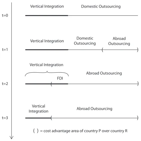
(36) up threads less credible because they provide entrepreneurs with more easily accessible outside options. For instance, if a partner threatens to withdraw from production, an efficient credit market might well mean that the threatened partner is able -or at least have more chances- to buy and/or build the machineries to internally produce the missing component. In other words, “with capital easy to come by, alienable assets such as plant and equipment have become less unique” (Rajan and Zingales (2001)). This means that physical investment is less relation-specific as a consequence of more efficient financial markets. Ideally, with perfect financial markets, no hold up may be based on any asset which could be possibly borrowed. In terms of the model the development of financial markets can be formalized as an increase of 𝛼. Moreover, it is likely that efficient credit markets are worth most to firms producing complex products which have very specific investments. Thus, if any, 𝛽 should decrease as financial markets become more efficient. Which means that the degree of vertical integration tends to diminish as a consequence of financial development. Industries comparison. The model predicts that complex products requiring hightech and sophisticated machinery are produced in industries whose structure tends to be more vertically integrated. In fact, one can interpret the parameter 𝛽 as a proxy for technology intensity or complexity. A sophisticated or complex final product involves a relatively large number of sophisticated intermediate products which require investment in highly specific machinery: this corresponds to a high 𝛽 (see Figure 2.3). A relatively standard product, on the contrary, involves relatively fewer complex stages of production, with less specific investments: this corresponds to a small 𝛽. Thus, technology intensive products will be produced by more integrated industries than standard products. Evidence of the above is very neatly provided by Novak and Eppinger (2001) who explicitly test the hypothesis that product complexity and vertical integration are complements. More evidence has been provided by Wilson (1977) who finds that licensing is more attractive the less complex the good involved is, and by Kogut and Zander (1993) whose results show that the probability of internalization is lower the more codifiable, teachable, and the less complex the technology is. North-South differences. As a consequence of the previous point, poor countries, producing less technology intensive products than rich countries, tend to have a lower number of vertical conglomerates. This is consistent with the observation that the economies of poor countries are generally characterized by household-style, non integrated firms. USA vs. Japanese keiretsu. Various authors (Spencer and Qiu (2001); Qiu and Spencer (2002)) have studied the case of the Japanese keiretsu and the reluctance of such conglomerates to import auto parts from abroad. They stress the fact that the Japanese import only parts of limited technological content, such as seat covers. The 27.