Universitat Polit`ecnica de Catalunya
Departament de Llenguatges i Sistemes Inform`atics
Programa de Doctorat en Computaci´o
PhD Dissertation
Geometric constraint solving
in a dynamic geometry framework
Marta R. Hidalgo Garcia
Advisor Robert Joan Arinyo
Acknowledgements
La reconnaissance est la memoire du coeur.
Jean Baptiste Massieu
En primer lloc vull agra¨ır de tot cor a Robert Joan tota l’ajuda i dedicaci´o que sempre m’ha prestat. Ha sabut guiar-me fins al final d’aquest llarg cam´ı. Vull agra¨ır tamb´e a la resta del grup de recerca per les xerrades junts i els consells que sempre han estat disposats a donar-me.
Gr`acies a Dominique Michelucci per acollir-me a Dijon i donar-me l’oportunitat de treballar al seu laboratori. Gr`acies tamb´e a tots els companys del laboratori Le2i i als companys de despatx Jean-Marc, Arnaud, Tomas, Abdoulaye, i en especial a George, Vishal, Cyril i Laureline per fer la meva estada molt m´es agradable.
M’agradaria donar les gr`acies a Enrique Zuazua i a Francisco Palacios per confiar en mi i deixar-me formar part del seu projecte. Segurament, aquesta tesi va comen¸car gr`acies a ells. Tamb´e a tots els companys de l’IMDEA Matem´aticas, en especial a F´atima, Jos´e Mar´ıa, Markus i Sebastian.
Vull tamb´e donar les gr`acies a tots els professors que he tingut des de petita i que m’han ensenyat a estimar les seves assignatures. En especial a Vicent Teruel per descobrir-me les matem`atiques i a Joan L. Monterde per ensenyar-me la bellesa de la geometria. Vull agra¨ır especialment a Manolo Sanchis tota la seva ajuda i suport a l’hora de fer la meva tesis de M`aster.
Gr`acies a tota la secci´o del Departament de Llenguatges i Sistemes Inform`atics per acollir-me i fer-me sentir una m´es del grup, i als companys de despatx que he tingut durant aquests anys: Eduard, Eloi, Irving, Jon`as, Marc, Pasku, Sergio i en especial a Sergi, per ser un amic a m´es d’un company tot aquest temps.
Gr`acies a tots els meus amics. A Mireia i Helena per voler estar sempre en el mateix metre quadrat que jo. A Eva, per estar cada dilluns a l’altre costat de l’Skype. A Natalia i Pili i la resta de companys del cineclub. A `Angels, Marina, Rafel, les dues Maries, Alfonso, Marta i en especial a Carlos, per l’any inoblidable que vam passar junts a Mainz. A Joan i Gabo i la resta de companys de Matem`atiques. A Anna i Jaume per estar ah´ı des de petits. I a tota la resta de gent que m’ha recolzat i m’ha deixat formar part de la seva vida.
Vull donar les gr`acies a tota la meva fam´ılia, dispersada per tota la geografia espanyola des de Vigo fins a Motril, passant per El Bonillo, Caudete, La Vila Joiosa i els voltants de Val`encia. En especial a Rosario, que em va obrir les portes de sa casa, i a les meves `avies Rosa i Fina, dones treballadores en temps dif´ıcils, per l’exemple que m’han donat.
Vull agra¨ır especialment als meus pares haver-me recolzat en totes les decisions que he pres en la meva vida, per dif´ıcils que els resultaren. Mai els podr´e estar suficientment agra¨ıda.
Per ´ultim vull donar les gr`acies a Toni per confiar sempre en mi, perqu`e s´e que sense ell aquesta tesi no haguera existit. I per donar alegria i pau a la meva vida cada dia.
Abstract
Geometric constraint solving is a central topic in many fields such as parametric solid modeling, computer-aided design or chemical molecular docking. A geometric constraint problem consists of a set geometric objects on which a set of constraints is defined. Solving the geometric constraint problem means finding a placement for the geometric elements with respect to each other such that the set of constraints holds.
Clearly, the primary goal of geometric constraint solving is to define rigid shapes. However an interesting problem arises when we ask whether allowing parameter constraint values to change with time makes sense. The answer is in the positive. Assuming a contin-uous change in the variant parameters, the result of the geometric constraint solving with variant parameters would result in the generation of families of different shapes built on top of the same geometric elements but governed by a fixed set of constraints. Considering the problem where several parameters change simultaneously would be a great accomplish-ment. However the potential combinatorial complexity make us to consider problems with just one variant parameter. Elaborating on work from other authors, we develop a new algorithm based on a new tool we have called h-graphs that properly solves the geometric constraint solving problem with one variant parameter. We offer a complete proof for the soundness of the approach which was missing in the original work.
Dynamic geometry is a computer-based technology developed to teach geometry at secondary schools. This technology provides the users with tools to define geometric con-structions along with interaction tools such as drag-and-drop. The goal of the system is to show in the user’s screen how the geometry changes in real time as the user interacts with the system. It is argued that this kind of interaction fosters students interest in experi-menting and checking their ideas. The most important drawback of dynamic geometry is
that it is the user who must know how the geometric problem is actually solved. Based on the fact that current user-computer interaction technology basically allows the user to drag just one geometric element at a time, we have developed a new dynamic geometry approach based on two ideas: 1) the underlying problem is just a geometric constraint problem with one variant parameter, which can be different for each drag-and-drop operation, and, 2) the burden of solving the geometric problem is left to the geometric constraint solver.
Two classic and interesting problems in many computational models are the reachability and the tracing problems. Reachability consists in deciding whether a certain state of the system can be reached from a given initial state following a set of allowed transformations. This problem is paramount in many fields such as robotics, path finding, path planing, Petri Nets, etc. When translated to dynamic geometry two specific problems arise: 1) when intersecting geometric elements were at least one of them has degree two or higher, the solution is not unique and, 2) for given values assigned to constraint parameters, it may well be the case that the geometric problem is not realizable. For example computing the intersection of two parallel lines. Within our geometric constraint-based dynamic geometry system we have developed an specific approach that solves both the reachability and the tracing problems by properly applying tools from dynamic systems theory.
Finally we consider Henneberg graphs, Laman graphs and tree-decomposable graphs which are fundamental tools in geometric constraint solving and its applications. We study which relationships can be established between them and show the conditions under which Henneberg constructions preserve graph tree-decomposability. Then we develop an algorithm to automatically generate tree-decomposable Laman graphs of a given order using Henneberg construction steps.
Contents
Acknowledgements i
Abstract iii
List of Figures ix
1 Introduction 1
1.1 Goals . . . 3
1.2 Scientific contributions . . . 4
1.3 Organization of the work . . . 4
2 Preliminaries 7
2.1 Graphs . . . 8
2.1.1 Connection of graphs . . . 10
2.1.2 The shortest path problem and the A∗
algorithm . . . 10
2.2 Geometric constraint problems . . . 11
2.2.1 Formal definition and properties . . . 11
2.2.2 Constructive geometric constraint problems solving . . . 15
2.3 Problems with one variant parameter . . . 18
2.3.1 The construction plan as a function . . . 18
2.4 Dynamic geometry . . . 23
2.4.1 Basic concepts on dynamic geometry . . . 23
2.4.2 Constraint-based dynamic geometry . . . 25
3 The hinges graph 31 3.1 Dependency between tree-decomposition steps . . . 31
3.2 Definition of the hinges graph . . . 35
3.3 H-graph from a construction plan . . . 37
3.4 Subgraphs and complete subgraphs . . . 39
3.5 Representative nodes of complete subgraphs . . . 41
3.6 Conclusions . . . 47
4 Parameter ranges 49 4.1 Preliminaries . . . 50
4.1.1 The domain of a geometric constraint problem with a variant parameter 50 4.1.2 Dependence on the variant parameter . . . 51
4.1.3 Dependence and h-graphs . . . 52
4.2 The van der Meiden method . . . 55
4.2.1 Computing the candidate points . . . 56
4.2.2 Computing the domain . . . 57
4.2.3 Limitations of the method . . . 58
4.3 Our implementation . . . 59
4.4 Algorithm correctness . . . 62
4.4.1 The transformation . . . 62
4.4.2 The set of solution instances . . . 63
4.4.3 Correctness . . . 66
4.5 Case study . . . 67
4.6 Conclusions . . . 72
5 The reachability problem 75 5.1 Continuity and continuous transitions . . . 76
5.1.1 Continuity . . . 76
5.1.2 Continuous transitions . . . 77
5.1.3 Case study: the four-bars linkage . . . 80
5.2 An algorithm for the reachability problem . . . 87
5.2.1 The transitions graph . . . 88
5.2.2 Deciding reachability . . . 94
5.3 Implementation and results . . . 101
5.4 Conclusions . . . 105
6 The tracing problem 107 6.1 Definition of the tracing problem . . . 108
6.2 Solution to the tracing problem . . . 110
6.2.1 Previous approaches . . . 110
6.2.2 An approach to the solution of the tracing problem . . . 110
6.2.3 On continuity and determinism . . . 112
6.3 Implementation . . . 115
6.4 Conclusions . . . 117
7 Henneberg graphs and tree-decomposability 121 7.1 Henneberg families and tree-decomposable graphs . . . 122
7.1.1 Henneberg steps and Henneberg families . . . 122
7.1.2 A characterization of tree-decomposable Laman graphs . . . 124
7.1.3 Inclusion relations . . . 127
7.2 Preserving tree-decomposability in Henneberg steps . . . 129
7.2.1 Henneberg I steps and tree-decomposition . . . 130
7.2.2 Henneberg II steps and tree-decomposition . . . 130
7.3 An algorithm to generate tree-decomposable graphs . . . 137
7.3.1 Henneberg constructions and h-graphs . . . 137
7.3.2 Maximal Laman subgraph in h-graphs . . . 142
7.3.3 The algorithm . . . 143
7.4 Conclusions . . . 147
8 Conclusions and future work 151 8.1 Conclusions . . . 151
8.2 Future work . . . 154
List of Figures
2.1 Different kinds of graph. a) Graph. b) Simple graph. c) Partially directed
graph. . . 9
2.2 Subgraphs. a) Graph with vertices {A,B,C,D,E,F,G}. b) Subgraph of the graph depicted in a). c) Subgraph of the graph depicted in a) induced by the set of vertices V′ ={B,C,D,E,F}. . . 9
2.3 Geometric constraint problem example. a) Geometric sketch. b) Geometric constraint problem abstracted as a graph. . . 14
2.4 Construction plan for the example problem in Figure 2.3. . . 16
2.5 Sibling clusters pairwise share one geometric element. . . 16
2.6 Construction plan as a tree decomposition. . . 17
2.7 Geometric constraint problem with one variant parameter λ. . . 19
2.8 Objects belonging to the family defined by the problem in Figure 2.7. From left to right, T(σ,2.5), T(σ,4.5) and T(σ,5.9). . . 20
2.9 Critical values for a triangle defined by two sides and the angle supported by one of them. Construction plan and actual construction. . . 21
2.10 Example of GSP. Left) A GSP. Right) A GSP instance. . . 24
2.11 Geometric problem in Figure 2.10 expressed as a geometric constraint solving problem. . . 27
2.12 An architecture for the constructive solving technique. . . 28
3.1 Dependence. a) Scheme of two directly dependent problems. b) Scheme of two indirectly dependent problems. In this case, problem with hinges (u1, v1, w1) depends indirectly on the problem with hinges (u2, v2, w2). c) Scheme of two independent problems. . . 32
3.2 Strong dependence. a) Strong dependence in the case that T2 contains a hinge of T1. b) Strong dependence in the case that a tree-decomposition step T3 in which T2 depends indirectly contains a hinge of T1. . . 34
3.3 Example of h-graph. a) Tree-decomposable Laman graph G. b) h-graph
H(G) associated toG. . . 36
3.4 Complete subgraph. a) H-graph H(G′
) which is a subgraph of the h-graph depicted in Figure 3.3b. b) Tree-decomposable Laman subgraph G′
associ-ated to H(G′
), which is a subgraph of the graph depicted in Figure 3.3a. . . 42
3.5 Illustration of Theorem 3.5.5. a) The minimum subgraphGu,v includingu, v
is included in the clusterG1which containsuandv. b) Tree-Decomposition Step (u, v, w) depends indirectly on every tree-decomposition step inGu,v. . 44
4.1 Dependency of a construction step. a) Directly dependent. b) Indirectly dependent. c) Independent. . . 51
4.2 Dependence on the variant parameter. a) Graph G representing the geo-metric constraint problem Πλ. b) H-graph H(G) associated to G. . . 54
4.3 Candidate points computation process for indirectly dependent tree-decom-position steps. a) Tree-decomtree-decom-position step that depends indirectly onλ. b) Transformed problem that depends directly on µ. c) Construction where values for the variant parameter λare measured. . . 57
4.4 Relation between the values of the variant parameter λand the values ofµ. 58
4.5 In well-constrained problems which indirectly depend on the variant param-eter λ, the only two possible locations for λ are shown in this Figure. a) The variant parameter is defined upon two elements different to the hinges
u′
, v′
. b) The variant parameter is defined upon one of the hinges, say u′
, and another arbitrary element different to the other hinge v′. . . . 63
4.6 Two problems defined over the same set of geometric objects. a) Problem Π1. b) Problem Π2. . . 65
4.7 Solution instances. a) Instance for problem Π1. b) Instance for problem Π2. 65
4.8 Case study. a) Piston and connecting rod crankshaft. b) Geometric abstrac-tion. c) Construction plan. . . 68
4.9 Piston and connecting rod crankshaft. a) Problem graph G. b) Tree-decomposition of the problem. c) Associated h-graph H(G). . . 69
4.10 Piston and connecting rod crankshaft. Transformed problem. a) Problem graph. b) Decomposition tree of the problem. c) Associated h-graph H(G′
). 70
4.11 Piston and connecting rod crankshaft. Transformed problem. a) Construc-tion plan. b) Geometric realizaConstruc-tion. . . 70
4.12 Construction of the transformed problem. a) Construction at µ = 3. b) Construction at µ= 13. . . 71
4.13 Feasibility for the piston and connecting rod cranckshaft problem. • rep-resent critical points. |represent intermediate λ values. X means that the
construction plan is feasible. ×means that the construction plan is unfeasible. 71
4.14 Piston and connecting rod crankshaft. Feasible domain for the variant pa-rameterλ=d2. . . 72
5.1 Domain intervals of the domain of a geometric constraint problem. . . 78
5.2 Four-bars linkage problem scheme. . . 80
5.3 Instances of the four-bars linkage. a) The four-bars linkage for a value of
α = 0. b) The four-bars linkage for a value of α = π/2. c) The four-bars linkage for a value of α=π. . . 81
5.4 Case 1. a) Solution instance at value α=α0. b) Domain of the problem. . 83
5.5 Case 2. a) Solution instance at value α=α0. b) Domain of the problem. . 83
5.6 Case 3. a) Solution instance at value α=α0. b) Domain of the problem. . 83
5.7 Case 4. a) Solution instance at value α=α0. b) Domain of the problem. . 84
5.8 Case 5. a) Solution instance at value α=α0. b) Domain of the problem. . 84
5.9 Case 6. a) Solution instance at value α=α0. b) Domain of the problem. . 85
5.10 Case 7. a) Solution instance at valueα=α0. b) Domain of the problem. . 85
5.11 Particular case of the four-bars problem. a) Configuration forα =π/2. b) Domain. c) Simplified domain. . . 86
5.12 Particular case. a) Instance of the problem in Figure 5.11a at variant pa-rameter value α= 0. b) Split domain. . . 87
5.13 Domain for the fourbars problem withd0 =d2 = 5 and d1 =d3= 4. . . 88
5.14 Domain represented as a bucket sort table of intervals. . . 90
5.15 Transitions graph for the example in Figure 5.1. . . 92
5.16 Domain and continuous transitions of a geometric problem. Continuous transitions are represented as arrows between endpoints of the domain in-tervals. . . 93
5.17 Transitions graph for the domain in Figure 5.16. . . 93
5.18 Extended transitions graph derived from the transitions graph in Figure 5.17 after adding the starting and ending vertices. . . 95
5.19 Schematic representation of a path solving the reachability problem from vertexVsto vertexVe. No optimal path between verticesVs andVe includes
the dashed line. . . 95
5.20 Angle variant parameters. Three possible configurations giving rise to three different values for the minimum distance covered by a path from the current vertex with parameter value λto the final vertex with parameter valueλe. . 99
5.21 Two minimum paths output by Algorithm 10 that solve the reachability problem in Figure 5.16. Is = T(5, σ1) and Ie = T(5, σ4). Grey vertices represent the path, and white vertices are the not visited vertices. . . 101
5.22 Geometric constraint problem with six points and nine point-point distances. a) GraphG. b) h-graph H(G) associated to G. . . 102
5.23 Construction plan given by the constructive geometric constraint solver for problem in Figure 5.22. . . 103
5.24 Domain of the variant parameter of the problem in Figure 5.22. The set of continuous transitions betweene intervals are displayed as arrows. . . 103
5.25 Transitions graph of the problem in Figure 5.22. . . 104
5.26 Extended transitions graph for the reachability problem with initial instance
Is=T(0.5, σ4) and ending instanceIe=T(0.5, σ2). . . 104
5.27 Minimum path computed by the system for the reachability problem with initial instanceIs=T(0.5, σ4) and ending instanceIe=T(0.5, σ2). . . 105
6.1 Scheme of the given (check marks) and on demand (question marks) infor-mation in the tracing and the reachability problems. From Denner-Broser, [16]. . . 108
6.2 Definition of the tracing problem by means of a scheme . . . 111
6.3 Solution to the tracing problem corresponding to the solution to the reach-ability problem in Chapter 5, Section 5.3 . . . 112
6.4 Another solution to the tracing problem traversing only two intervals. . . . 113
6.5 Other solution to the tracing problem which associates to every point in the variant parameter path the same index assignment. . . 113
6.6 Bisector and double bisector. a) Possible bisectors of the angleα. b) Values of the angle, bisector and double bisector for the four different assignments of the problem with two bisectors. . . 114
6.7 Four possible configurations for the double bisector, allowing determinism and continuity. From left to right and from top to bottom, solution instances corresponding to index assignmentsσ1, σ2, σ3 and σ4 are shown. . . 116
6.8 The domain of the hypothetic problem with two bisectors. . . 116
6.9 The reachability simulator window at the initial instance of the simulation. 118
6.10 From left to right and from top to bottom, different instances in the tracing path for the tracing problem considered. The upper left image corresponds to the initial instance and the lower right image to the final one. . . 119
7.1 Henneberg I step. a) Graph G. b) Graph G∗ derived from graphGby the
application of a HS1. . . 123
7.2 Henneberg II step. a) Graph G. b) GraphG∗
derived from graph Gby the application of a HS2. . . 123
7.3 Merging of graphs A, B, C giving rise to graph D, with hingesa, b, c. . . 125
7.4 Counterexamples. a) Tree-decomposable Laman graph which cannot be constructed using only HS1. b) Non tree-decomposable LamanHII graph. . 128
7.5 Henneberg sequence leading to the Laman graph in Figure 7.4b which is not tree-decomposable, represented from left to right and from top to bottom. . 129
7.6 Necessary tree-decomposition step for the preservation of the tree-decom-posability in Henneberg II steps, Theorem 7.2.9. . . 132
7.7 Illustration of Theorem 7.2.9. a) Graph G∗
2 resulting after the merging of graph G2 with two edge graphs. b) Graph G∗∗2 resulting after the merging of graphG∗
2 with an edge graph andG3. . . 133
7.8 Illustration of Theorem 7.2.9. a) Case in whichv1, v2are in the same cluster. b) Case in whichv1, v2 are in different clusters. . . 134
7.9 Illustration of Theorem 7.2.9. a) A graph G which does not fulfill Laman condition. b) Tree-decomposable Laman graph G. . . 134
7.10 Illustration of Theorem 7.2.10. a) Graph resulting after the merging of
G2 with two edge graphs. b) Tree-decomposition step of a graph after the application of a HS2 involving elements v1, v2, v3. c) Construction of G by applying a HS1 adding vertex v2. . . 136
7.11 Application of a HS1. a) Resulting graphG∗
after adding vertexkand edges (b, k),(k, j) to the graph in Figure 3.3a. b) h-graph H(G∗) associated to G∗. 138
7.12 Application of a HS2. a) h-graphs associated to the remaining maximal tree-decomposable Laman subgraphsM1, M2. b) GraphM2′ after the application of the two indicated HS1. c) h-graph associated toM′
2,H(M
′
2). . . 142
7.13 Application of a HS2. a) Resulting graphG∗
after removing edge (a, h) and adding vertex k and edges (a, k),(g, k),(h, k) to the graph in Figure 3.3a. b) h-graph H(G∗) associated toG∗. . . . 143
7.14 Construction ofG′
by means of the original Hennberg II step (left), and by means of the alternative Henneberg I sequence (right). . . 146
CHAPTER
1
Introduction
The reachability problem is a fundamental issue in the context of many models and ab-stractions which describe different computational processes. Analysis of the computational traces and predictability questions for such models can be formalized as a set of different reachability problems. Reachability can be formulated in general as
Given a computational system with a set of allowed transformations, also called functions, decide whether a certain state of a system is reachable from a given initial state by a set of allowed transformations.
A huge amount of literature on reachability have been published mainly in the field of abstract computational models see for example [10]. Examples of classical fields where the reachability problem is considered are graphs theory, [14, 93, 95, 111], Petri nets, [80, 81, 85, 110], motion planning,[54, 76, 77], geographical navigation,[2, 3, 32, 92] and robotics, [69, 77, 109, 112]. A feature common to most of the referred works deal with systems the behavior of which can be basically captured by identifying a set of well-defined discrete states.
2 Introduction
high resolution color screens for user-computer interaction. The key concept in dynamic geometry is interaction, that is, select a geometric object in the screen, move it and see immediately how the geometric construction changes.
Compared to ruler-and-compass drawings on the paper, dynamic geometry systems offer two clear advantages. First they provide tools to create accurate drawings (intersection points, tangencies, etc). Second the computer can record the way the user constructed the geometric elements that allows it to quickly rebuild the construction every time the user changes the values assigned to some parameters. As a consequence, exploration and experimentation are encouraged by showing to the user which parts of the construction change and which remain unchanged.
In this context, a reachability problem naturally arises and can informally be stated as follows.
LetIsandIebe two instances of a well defined geometric construction whereIs
is called the starting instance andIe the ending instance. Are there continuous
transformations that, preserving the incidence relationships established in the geometric construction, bringsIs toIe?
Now the scenario is different from the one described above. Notice that in dynamic geometry no set of well defined states can be identified. Moreover, the reachability problem in dynamic geometry belongs to a continuous domain.
A problem in dynamic geometry tightly related to the reachability problem is thetracing
problem which can be informally defined as
Let Is and Ie be two specific instances of a well defined geometric
construc-tion where Is is called the starting instance and Ie the ending instance. Let I0, I1, . . . , Ii, . . . , In be a sequence of well defined geometric constructions such
that Ii+1 is a continuous incremental variation of Ii which preserves incidence
relationships. If we setI0=Is, does the sequence of incremental constructions
end at In=Ie?
When using current dynamic geometry systems, the user can find that strange things happen from time to time. An object might suddenly jump into a different position or disappear completely or a group of objects may converge to the same position. It turns out that these effects are caused by a number of non-trivial mathematical issues. Since they have a dramatic effect on both reachability and tracing in dynamic geometry, they must be properly addressed.
1.1 Goals 3
the fact that, in general, geometric operations have more than one solution, for example, intersecting a line and a circle. Another ambiguity appears when a problem with a well-defined solution whenever geometric elements are in general position, say computing the point where two straight lines intersect, reaches a degenerate configuration, for example, the straight lines became parallel.
Examples of unfeasibility of the geometric construction appears whenever solving the equations underlying the geometric problem requires dividing by zero or computing square roots of negative values. The set of parameter values where constructions are unfeasible are called critical points.
In order to work out a satisfactory solution for both the reachability and tracing prob-lems in dynamic geometry a well-defined method for handling both ambiguities and geo-metric unfeasibility must be found.
There is a paucity of works concerning reachability and tracing problems in dynamic geometry. Richter-Gebert and Kortenkamp in [90] formalized the reachability problem in computational geometry and proved that its complexity is NP-hard in R. To deal with
the tracing problem, authors describe a method based on applying a detour to the tracing whenever it gets close to conditions that, according to numerical heuristics, are close to critical points.
In [15, 16], Denner-Broser describes a decision algorithm to solve the reachability prob-lem in dynamic geometry using Voronoi diagrams. In a first step the algorithm computes the Voronoi diagram defined by the sites corresponding to critical points. The reachability problem is solved by checking whether there is a path of Voronoi edges connecting the starting and ending points in the Voronoi partition associated to the starting and end-ing geometric instances such that avoids the Voronoi sites. However, no evidences of any implementation are given.
1.1
Goals
The main goal of this thesis is to establish a theoretical framework to solve the reachability and tracing problems in dynamic geometry.
4 Introduction
1.2
Scientific contributions
The scientific contributions of this work belong to one of two categories: Basic tools and main goals. Among the basic tools we find
h-graphs : We introduce a new representation for tree-decomposable Laman graphs, which we call h-graphs, which includes the information about its tree-decomposition and presents some nice properties. H-graphs are used with different purposes in this work.
van der Meiden soundness : We describe in detail the method to compute the domain of a geometric constraint problem with one degree of freedom reported by van der Meiden in [105]. We formalize the underlying concepts and prove for the first time that the method is correct.
Henneberg graphs : We establish some relationships between Henneberg graphs, tree-decomposable graphs and Laman graphs. We then develop a correct algorithm which computes tree-decomposable Laman graphs of a given size using Henneberg construc-tions. Here h-graphs play a central role.
Contributions to the main goals are
Reachability : We define a theoretical framework to solve the reachability problem in dynamic geometry. We show that the approach is correct and that it finds a solution whenever one exists. We develop a specific implementation in the framework of a dynamic geometry system based on constructive geometric constraint solving.
Tracing : We develop a solution to the tracing problem as a derivation of the solution to the reachability problem. The approach is implemented as a unit in our dynamic geometry system.
1.3
Organization of the work
This thesis includes eight chapters organized in four main parts. First, in Chapter 2 we introduce the basic concepts used in subsequent chapters. We recall elementary definitions on graphs, geometric constraint problems and dynamic geometry.
1.3 Organization of the work 5
problem and the associated tree-decomposition. Later on in this work, h-graphs will play a central role.
The third part includes Chapters 4, 5 and 6. It is devoted to solve the reachability and tracing problems in geometric constraint-based dynamic geometry. In Chapter 4 we prove for the first time that the van der Meiden approach to compute critical points is correct. Then we describe our own implementation based on h-graphs. In Chapter 5 we develop our approach to solve the reachability problem in dynamic geometry. A proof of the optimality of the searching algorithm is presented. We describe the prototype implemented on top of our geometric constraint-based dynamic geometry system. Chapter 6 describes our solution to the tracing problem. Some remarks about continuity in our system are highlighted. The implementation on top of our geometric constraint-based dynamic geometry system is also described.
The last part of this work includes Chapter 7. Here we develop a correct method to automatically build tree-decomposable Laman graphs of a given size using Henneberg constructions. The approach heavily relays on h-graphs.
CHAPTER
2
Preliminaries
Now, in order to answer the question, ”Where do we go from here”
which is our theme, we must first honestly recognize where we are now.
Martin Luther King
In this chapter we review some basic facts about graphs, geometric constraint solving and dynamic geometry which we will use in this work. Readers already familiarized with these fields may skip it, although we shall refer to the concepts presented here all along the manuscript.
8 Preliminaries
2.1
Graphs
Although we assume that most of the readers are already acquainted with the issues ad-dressed in this section, we introduce now the main topics on graphs due to the key role they play all along this work. Both the outlined problems, and the proposed solutions are abstracted as graphs.
The information in this section is commonly known and can be found in many books on this topic, for example books in references from [6] and [33]. You can also see [13]. We will focus on the main features of the particular class of graphs concerned in this work.
A graph can be seen as a diagram consisting of a set of vertices, also called nodes, together with lines joining certain pairs of these vertices. For example, the vertices could represent airports, and the lines the flights connecting them. Graphs are mathematical abstractions of this kind of situations. More precisely,
Definition 2.1.1
A graph G is an ordered pair(V, E) consisting on a nonempty set of vertices V and a set of edges E. Elements in E are pairs of elements of V, not necessarily distinct, called the endpoints of the edge.
Graphs are so named because they can be represented graphically, and it is this graph-ical representation which helps us to understand many of their properties. Each vertex is indicated by a point, and each edge by a line joining the points which represent its end-points. Figure 2.1 shows a collection of graphs. Their vertices are A, B, C, D, E, F, G, and H.
There is not a unique way of drawing a graph, as the relative positions of points representing vertices and lines representing edges have no significance. We shall, however, often draw a diagram of a graph and refer to it as the graph itself.
If vertexv∈V is an endpoint of edge e∈E, thenv is said to be incidenton e, ande
is incident on v. An edge is said to joinits endpoints, and a vertex is adjacentto another vertex if they are joined by an edge. The notation V(G) and E(G), or VG and EG, will
be used for the vertex and edge sets respectively in case that G is not the only graph in consideration.
When the endpoints of an edge are the same vertex, the edge is said to be aloop. When they are different, the edge is said to be a proper edge. A multi-edgeis a collection of two or more edges having identical endpoints. A simple graphis a graph that has no loops or multi-edges. Notice that graph in Figure 2.1b is a simple graph, for it has no loops nor multi-edges. In this work, we shall only consider simple graphs.
2.1 Graphs 9 A B C D E F G H z s y w x v u t p o q r A B C D F G w x u t o r
p y H
E A B C D E F G H z s y w x v u t p o q r
a b c
Figure 2.1: Different kinds of graph. a) Graph. b) Simple graph. c) Partially directed graph.
and whose other endpoint is designated as thesink vertex. They are denotedsource(e) and
sink(e), respectively. Directed edges are usually denoted by an arrow. Edges for which this distinction does not exist are called undirected. A directed graph is a graph whose edges are directed. Analogously, an undirected graph is a graph whose edges are undirected. A
partially directed graph, is a graph that has undirected and directed edges. Graphs in Figures 2.1a and 2.1b are undirected and Figure 2.1c shows a partially directed graph, for some of its vertices are directed and some others not.
The degree of a vertex v ∈ V in a graph G, denoted deg(v), is the number of proper edges incident on v plus twice the number of loops. For simple graphs, which are our subject of study, the degree is simply the number of adjacent vertices.
A graph H is a subgraph of G, written H ⊆ G, if V(H) ⊆ V(G) and E(H) ⊆ E(G). In this case, G is a supra-graph of H. Assuming that V′ is a nonempty subset of V, the
subgraph ofGwhose vertex set isV′
and whose edge set is the set of those edges ofGthat have both ends in V′
is called the subgraph of Ginducedby V′
and is denoted by G[V′
]. A B C D E F G z y x w v u t s r p q A B C D E
F y G v u t p q B C D E F x w v u t s r
[image:27.612.130.518.502.591.2]a b c
Figure 2.2: Subgraphs. a) Graph with vertices {A,B,C,D,E,F,G}. b) Subgraph of the graph depicted in a). c) Subgraph of the graph depicted in a) induced by the set of verticesV′
10 Preliminaries
Figures 2.2b and 2.2c show two graphs which are subgraphs of the graph depicted in Figure 2.2a. Figure 2.2a is then a supra-graph of the graphs in Figures 2.2b and 2.2c. Figure 2.2c is also the subgraph induced by the set of vertices{B, C, D, E, F}.
2.1.1 Connection of graphs
A walk in G is a finite non-null sequence W =v0e1v1e2v2. . . ekvk, whose terms are
alter-nately vertices and edges, such that, for 1≤i≤k, the ends of ei are vi−1 and vi. We say
thatW is a walk fromv0 tovk. The integerkis thelengthofW. In a simple graph, a walk
is determined by the sequence of its vertices. If the edges of a walk W are distinct and also the vertices are distinct, thenW is called apath. We shall also use the word ’path’ to denote a graph or subgraph whose vertices and edges are the terms of a path.
Two verticesu andv ofG are said to be connected if there is a path inGfromu tov. Connection is an equivalence relation on the vertex set V. Thus there is a partition of V
into nonempty subsets V1, V2, . . . , Vω such that two vertices u and v are connected if and
only if bothu and v belong to the same set Vi. The subgraphs G[V1], G[V2]. . . , G[Vω] are
called the connected components of G. If G has exactly one connected component, G is
connected. Otherwise, Gisdisconnected. Notice that a path is connected if between every pair of vertices there is a path. Thedistance between two vertices in a graph is the length of the shortest path between them.
Graphs in Figure 2.1 are all three disconnected, with two connected components each. Graphs in Figures 2.2a and 2.2c are connected, and the one depicted in Figure 2.2b is disconnected.
2.1.2 The shortest path problem and the A∗
algorithm
With each edge eofG let there be associated a real numberw(e), called its weight. Then
G, together with these weights on its edges, is called aweighted graph. In the airport graph example cited above, weights could represent the number of flights between each pair of airports. If H is a subgraph of a weighted graph, the weight w(H) of H is the sum of weights on its edges. The shortest path problem consists on finding, in a weighted graph, a path of minimum weight connecting two specified vertices. The weight of a path is also called itslength, and similarly the minimum weight of a path fromutovwill be also called thedistance betweenu and v inG.
A classic algorithm to solve the shortest path problem is the known as Dijkstra algo-rithm, [19], discovered by Dijkstra in 1959 and, independently, by Whitling and Hillier in 1960. For a complete review of the existing methods to solve the shortest path problem, see [93]. In this work we focus on the A∗
2.2 Geometric constraint problems 11
is complete and optimal under certain conditions. We describe the basics of this method following [91], where more information on this algorithm can be found.
The A∗ algorithm is based on the minimization of an evaluation function f which is
actually the sum of two other functions:
f(n) =g(n) +h(n)
whereg(n) is thepath-costfunction andh(n) an heuristic function. Theg(n) function gives the path cost from the starting node to the noden, and theh(n) function is the estimated cost of the cheapest path from node n to the goal. Then,f(n) is the estimate cost of the cheapest solution throughn.
In order the A∗
algorithm to be complete and optimal, function h(n) must never over-estimate the real cost to reach the goal. Such an h(n) is called an admissible heuristic. If h(n) is admissible, then f(n) never overestimates the actual cost of the best solution through n. A final observation is that among optimal algorithms of this type, A∗
is op-timally efficient, that is, no other optimal algorithm is guaranteed to expand fewer nodes than A∗
. A proof of this result appears in [14].
2.2
Geometric constraint problems
In this work we model the problems we deal with as geometric constraint problems. A geometric constraint problem is made of a set of different geometric objects, related by a set of constraints among them. Many different approaches have been reported to solve the geometric constraint problem. In this section we formalize the notion of geometric constraint problem, analyze different solutions already known and describe thoroughly the one known as constructive.
2.2.1 Formal definition and properties
Geometric constraint solving is arguable a core technology of computer aided design and, by extension, geometric constraint solving is also applicable in virtual reality and is closely related in a technical sense to geometric theorem proving. For solution techniques, geo-metric constraint solving also borrows heavily from symbolic algebraic computation and matroid theory.
12 Preliminaries
• ΠE is the geometric space constituting a reference framework into which the problem
is embedded. ΠE is usually Euclidean.
• ΠO is the set of specific geometric objects which define the problem. They are chosen
from a fixed repertoire including points, lines, circles and the like.
• ΠX is a, possibly empty, set of variables whose values must be determined. In
general, variables represent quantities with geometric meaning: distances, angles and so on. When the quantities are without a geometric meaning, for example, when they quantify technological aspects and functional capabilities, those variables are calledexternal.
• ΠC is the set of constraints. Constraints can be geometric or equational. Geometric
constraints are relationships between geometric elements chosen from a predefined set, e.g., distance, angle, tangency, etc. The relationship (the distance, the angle, ...) is represented by a tag. If the tag represents a fixed value, known in advance, then the constraint is calledvaluated. If the tag represents a value to be computed as part of solving the constraint problem, then the constraint is calledsymbolic, [43].
Equational constraints are equations some of whose variables are tags of symbolic constraints. The set of equational constraints can be empty.
The general geometric constraint solving problem can be now stated as follows:
Given a geometric constraint problem Π =<ΠE,ΠO,ΠX,ΠC >,
1. Are the geometric elements in ΠO placed with respect to each other in
such a way that the constraints in ΠC and equations in ΠX are satisfied?
If the answer is positive, then
2. Given an assignment of values to the valuated constraints and external variables, is there an actual construction that satisfies the constraints and equations?
When dealing with geometric constraint solving, the first issue that needs to be settled is the dimension of the embedding space ΠE. In 2D Euclidean space, ΠE =R2, a number
of techniques have been developed that successfully solve the geometric constraint solving problem. For an in-depth review see Jermann, [60]. However, there remain open questions such as characterizing the competence (also called domain) of the known techniques.
Spatial constraint solving, where ΠE = R3, include problems in fields like molecular
2.2 Geometric constraint problems 13
Pioneering work has been reported by Hoffmann and Vermeer, [49, 50] and by Durand, [20].
Presented in this way, the geometric constraint solving problem includes in general issues concerning how to deal with external variables. Here we refer the interested reader to the work by Hoffmann and Joan-Arinyo, [43], and Joan-Arinyo and Soto, [65].
The basic constraint problem only considers geometric elements and constraints whose tags are assigned a value. It excludes external variables, constraints whose tags must be computed, and equational constraints. So the basic problem is stated in the following way.
Given a set ΠO with n geometric elements and a set ΠC with m geometric
constraints defined on them
1. Is there a placement of the n geometric elements such that the m con-straints are fulfilled? If the answer is positive,
2. Given an assignment of values to themconstraints tags, is there an actual construction of the ngeometric elements satisfying the constraints?
In what follows we will focus on the basic geometric constraint solving problem.
Geometric constraint problems can be represented by a graph. The vertices shall rep-resent the geometric elements of the problem and the edges shall reprep-resent the constraints among them. Given a geometric constraint problem Π =< ΠG,ΠC,ΠP >, the graph G= (V, E) such thatV = ΠG,E= ΠC and the edges are labeled with the parameters ΠP
represents the problem Π. The graphGis a simple graph, because constraints are defined upon two different geometric objects (thus, no loops are allowed) and between any two objects there is no more than one constraint (thus, no multi-edges are allowed). G is also undirected, since relations among geometric objects are non oriented.
Figure 2.3a shows an example of geometric constraint problem consisting of six points
{a, b, c, d, e, f} and nine point-point distance constraints {di,1 ≤ i ≤ 9} defined among
them. Figure 2.3b shows the geometric constraint problem abstracted as a graph where each node represents one geometric element and each labeled edge represents a geometric constraint defined on the two geometric elements the edge connects. In what follows we shall represent geometric constraint problems as graphs.
14 Preliminaries d3 d d9 d4 d1 a b e d8 d2 d6 d7 d5 f a b e d f d9
d1 d2
d4 d8 d6 d7 d5 d3 a b
Figure 2.3: Geometric constraint problem example. a) Geometric sketch. b) Geometric constraint problem abstracted as a graph.
the number of solutions of the considered problem. In this context, geometric constraint problems are categorized in three different families:
1. Well-constrained problems are geometric constraint problems with a non-empty and finite set of solutions. In this work, we shall define rigid problems as well-constrained problems.
2. Over-constrained problems are those problems with no actual solution. Generally, the elimination of one or more constraints results in a well-constrained problem.
3. Under-constrained problems are geometric constraint problems for which an infinite set of solutions exists. Generally, the addition of one or more constraints results in a well-constrained problem.
Rigidity, as defined above, only refers to the problem’s structure, and no other questions are considered. However, inconsistent situations in which specific assigned values given to the parameters result in a change of category may arise. Some works concerning this topic are for example from Laman, [75], and the more recent ones from Fudos and Hoffmann,[28], Hoffmann et al., [43], Whiteley, [107], Henneberg [35] or Graveret al. [55].
As stated above, we identify well-constrained graphs with rigid graphs, that is, graphs which actually represent ruler-and-compass constructions. They are also known as Laman graphs after Gerard Laman, who first described them in 1970, [75]. Specifically, a graph
G= (V, E) is called Laman if|V| ≥3 and Gfulfills
2.2 Geometric constraint problems 15
2. For every subgraph G′
= (V′
, E′
) holds |E′
| ≤2|V′
| −3.
It is straightforward to see that Laman graphs have no disconnecting points and no vertices with degree zero nor one. An in depth discussion on Laman graphs will be presented in Chapter 7.
From now on, we will consider only well-constrained geometric constraint problems represented by undirected simple graphs, that is, graphs with no loops, no multi-edges and no direction established in their edges.
2.2.2 Constructive geometric constraint problems solving
Many techniques have been reported in the literature that provide powerful and efficient methods for solving geometric problems defined by constraints, which can be classified in three big groups: equational, based on the degree of freedom and constructive. For a complete review see [5, 45].
Equational methods are for example the numeric methods based on the Newton-Raphson algorithm [67], such as the systems described in [36, 78, 79, 82], or the algebraic symbolic methods which calculate the Gr¨obner basis of the equations system, like [12]. Methods based on the analysis of the degree of freedom are, among others, the works of Kramer, [71, 72, 73], or Hsu, [52, 53]. Among the constructive methods we find [8, 26, 27, 28], by Fudos
et al. or [102], by Todd.
Among all the geometric constraint solving techniques, our interest here focuses on the one known as constructive. For an in depth discussion on this topic see, for example, [1, 9, 11, 28, 47, 48, 59, 64, 66, 84, 101] and the references there in. Computer programs that solve geometric problems defined by constraints are called solvers.
Constructive solvers yield the solution to the geometric problem defined by constraints as a sequence of construction steps that places each geometric element with respect to each other in such a way that the constraints are fulfilled. This sequence is called the
construction plan. Construction plans represent a possibly exponential number of different solutions. In general, the construction plan that solves a constraint problem is not unique.
Figure 2.4 shows a construction plan for the constraint problem given in Figure 2.3. The meaning of each construction step is the usual. For example, origin() stands for the origin of an arbitrary framework,b=distD(a, d3) places pointbat distance d3 from point
a,c2 =circleCR(a, d1) defines the circlec2 with center aand radius d1 andintCC(c1, c2) defines a point as the intersection of circles c1 and c2. Notice that symbols ci do not
16 Preliminaries
[image:34.612.240.334.512.614.2]1. a = origin() 8. d =intCC(c4, c5, s2) 2. b = distD(a, d3) 9. c6 =circleCR(c, d6) 3. c2 = circleCR(a, d1) 10. c7 =circleCR(d, d7) 4. c3 = circleCR(b, d2) 11. e =intCC(c6, c7, s3) 5. c = intCC(c2, c3, s1) 12. c8 =circleCR(c, d9) 6. c4 = circleCR(a, d4) 13. c9 =circleCR(e, d8) 7. c5 = circleCR(d, d5) 14. f =intCC(c8, c9, s4)
Figure 2.4: Construction plan for the example problem in Figure 2.3.
Constructive solvers are also known as decomposition-recombination planners (DR-planners), [48], since they follow the following strategy: first, perform the decomposition of the problem at hand in a concrete way, then analyze the obtained decomposition and finally construct the solution by recombining the different parts.
We shall refer as decomposition step to the split of a graph G into three different subgraphsG1, G2, G3, calledclusters, in such a way thatG1∪G2∪G3 =GandG1∩G2 =
{h1}, G1∩G3={h2}, G2∩G3 ={h3}. Figure 2.5 illustrates the situation. Shared geometric elements h1, h2, h3 are called hinges. The set of three hinges of a tree-decomposition step shall be called triple of hingesor hinge triple. If the three clusters G1, G2, G3 include two vertices and one edge each, we say that the decomposition step is abasic step. For a more formal rational on this topic see [28] and [64].
If a graphGcan be decomposed by applying successively decomposition steps to each cluster until every subgraph contains only two vertices and one edge between them, we shall say that the graph G is tree-decomposable and that the successive decomposition steps are a tree-decomposition for G. We shall also say that the problem represented by the graphGis tree-decomposable by extension. Unfortunately, not all rigid graphs can be decomposed in such a way, and in those cases the method will fail. An in depth discussion
G1
G2
G3
h1
h3
h2
2.2 Geometric constraint problems 17
{e, d}
{f, e}
{b, c} {c, a}
{a, b, c}, s1 {d, b} {a, b, c, d}, s2
{a, b, c, d, e}, s3 {c, f} {a, b, c, d, e, f}, s4
{a, b}
{a, d}
[image:35.612.232.417.97.225.2]{c, e}
Figure 2.6: Construction plan as a tree decomposition.
on tree-decomposable graphs can be found in Chapter 7.
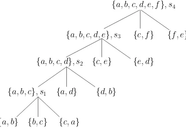
The tree-decomposition is a different and more convenient way to represent the con-struction plan, [66]. Figure 2.6 shows a decomposition tree for the concon-struction plan in Figure 2.4. Notice that sibling clusters pairwise share one geometric element, for example clusters {a, b, c, d, e},{f, e}and {c, f}pairwise share c,eand f respectively.
Once a graph has been decomposed, the tree-decomposition is used to construct a solution instance of the problem. Leaf nodes represent elemental placement problems corresponding to two geometric elements and the constraint defined on them. For example: two points at a given distance, a point and a straight segment at a given distance, two straight segments at a given angle and so on. The method starts by determining the position relative to each other of the two elements in a leaf node. Edges in the decomposition tree represent the combination of three solved clusters into a larger rigid cluster by application of a specific solving rule. Each node in the tree stands for a rigid object, built on the geometric objects included in the curly brackets list and whose position relative to each other has already been determined. The root node includes all the geometric elements in the problem and represents a solution instance.
In general, the tree-decomposition of a constraint problem is not unique. However, it has been proved that the tree-decomposition as defined above is canonical, [27, 64]. That means that the order in which the tree-decomposition is done is irrelevant, since they will always be the same decomposition steps. A consequence of that fact is that the hinge triples defined by the decomposition steps of a graph will always be the same, regardless of the concrete tree-decomposition at hand. That feature will give rise below to some interesting properties.
18 Preliminaries
Obviously, each specific root will result in a different placement for the geometric elements in the problem. Selecting the desired root is known as the root identification problem, firstly addressed in [9]. A number of techniques have been developed to deal with the root identification problem. See, for example, [9, 61, 62, 104].
With each root we associate a sign which will characterize unequivocally the corre-sponding solution. We will callindexto the set of all signs of a problem. The index in the construction plan in Figure 2.4 is I = {s1, s2, s3, s4}. For an in depth study of the index and the role it plays in geometric constraint solving see [24]. A similar definition can be found in [94]. The number of possible combinations of signs is bounded, as shown in [7].
The specific solution to the constraint problem Π identified by an assignment of values to the index I is called the intended solution. In what follows we consider that the intended solution has been fixed and that the degree of the equations underlying the geometric constraint problem is at most two, that is, signssi in the index take values in, say,{+,−}.
2.3
Problems with one variant parameter
When interacting with a computer featuring a mouse as an input device, mouse cursor position as it moves around the screen is captured in discrete steps. Therefore, intermediate positions are unknown. In dynamic geometry software, it is common practice to assume that the paths of free variables between two subsequent mouse events are linear, [70]. Thus, only one degree of freedom is left for the geometric element motion. In a more general framework, [15], the path is assumed to be polynomial in time t and the computation of the path itself is encoded leaving just one free variable tand in this way boiling down the problem to the situation with just one degree of freedom.
In this section we present basic concepts concerning geometric constraint problems for which the value of a given constraint parameter is not fixed, that is, geometric constraint problems with one variant parameter.
2.3.1 The construction plan as a function
In general, the concept of free geometric element in dynamic geometry can be captured in constructive geometric constraint-based dynamic geometry by considering the value assigned to a given constraint as a variable value. As we will see in Section 2.4.2, this does not have an effect on the constraint solving process and all what is needed is to reevaluate the construction plan as many times as needed.
2.3 Problems with one variant parameter 19
a
b e
d
f
d9
d1 d2
d4
d8
d6
d7
[image:37.612.272.379.98.219.2]d5 λ=d3
Figure 2.7: Geometric constraint problem with one variant parameterλ.
definition.
Definition 2.3.1
A geometric constraint problem with one variant parameter Π =<ΠG,ΠC,ΠP >is a well-constrained geometric constraint problem such that all parameters inΠP have been assigned a given value except for one, say λ, which can take arbitrary values in R.
The variant parameter may represent either a distance or an angle. We shall consider always positive distances, and angles defined inside the interval [−π/2, π/2]. Angles not included in this interval shall be wrapped to it moduloπ.
Let T be a construction plan which solves the constraint problem Π =<ΠG,ΠC,ΠP >.
Construction plans depend on the set of constraint parameters and on the index and they are valid for any problem derived from Π by considering one of its parameters as variant. Therefore, we can define the function construction plan as follows.
Definition 2.3.2
Let Π =< ΠG,ΠC,ΠP > be a geometric constraint problem and T a construction plan for Π. Then, T(σ, λ) represents the evaluation of the construction plan T for the index assignment σ and a value λ of the variant parameter.
Figure 2.8 shows from left to right objects in the family defined by the problem in Figure 2.7 for index value σ = {s1 = +, s2 = +, s3 = +, s4 = +}, distance constraint values d1 = 3, d2 = 3, d4 = 3.5, d5= 3.5, d6 = 4, d7 = 4.5, d8 = 4, d9= 3.5 and values of the variant parameter λin{2.5, 4.5, 5.9}. That is, T(σ,2.5), T(σ,4.5) and T(σ,5.9).
For some values of the variant parameterλ, however, it may not be possible to satisfy the set of constraints in ΠC, that is the construction plan T is unfeasible for such variant
20 Preliminaries
d
λ= 2.5
a b
c
e f
a b e
f
d c
λ= 4.5
a b e
f
c
d
λ= 5.9
a b c
Figure 2.8: Objects belonging to the family defined by the problem in Figure 2.7. From left to right, T(σ,2.5), T(σ,4.5) and T(σ,5.9).
or restricted versions of it have been addressed in the literature.
Shapiro and Vossler, [96], and Raghothama and Shapiro, [86, 87, 88], developed a theory on validity of parametric family of solids by investigating the relationship between Brep and CSG schemas in systems with dual representations for solid modeling. The formulation is built on formalisms of algebraic topology. Unfortunately, it seems a rather difficult problem transforming these formalisms into effective algorithms.
Joan-Arinyo and Mata [63] reported on a method to compute feasible ranges for pa-rameters in geometric constraint solving under the assumption that values assigned to parameters are non-trivial-width intervals. The method applies to complex systems of ge-ometric constraints in both 2D and 3D and has been successfully applied in the dynamic geometry field, [25]. It is a general method, the main drawback, however, is that it is based on numerical sampling.
Hoffmann and Kim [46] developed a constructive approach to calculate parameter ranges for systems of geometric constraints that include sets of isothetic line segments and distance constraints between them. Model instantiation for distance parameters within the ranges output by the method preserve the topology of the set of isothetic lines.
2.3 Problems with one variant parameter 21
1. a =origin() 2. b =distD(a, d1) 3. c1 =circleCR(b, d2) 4. l =lineP A(a, λ)
5. c =intCL(c, l, s) a d1 b
c′′ c′
d2
c λ
l
Figure 2.9: Critical values for a triangle defined by two sides and the angle supported by one of them. Construction plan and actual construction.
we shall prove that it is correct and complete, for it will be at the core of our approach to solve the reachability problem for geometric constraint based dynamic geometry.
Gao and Sitharam, in [29], described a general result concerning the computation of critical values for 2D problems with one degree of freedom which include just distance con-straints and such that can be abstracted as one degree of freedom Henneberg graphs. Here we consider problems including distance and angle constraints such that can be abstracted as tree decomposable graphs, a superset of Henneberg graphs.
To formalize concepts related to construction plan feasibility, we call critical variant parameter value, or simplycritical value, to the valuesλc of the variant parameter for which
the feasibility of T changes. For the same critical valueλc, a set of different constructions
can be made depending on the chosen index.
To illustrate critical values, consider the construction shown in Figure 2.9 where a triangle is defined by giving the constraints b = distD(a, d1), c = distD(b, d2), and λ =
angle(ab, ac). If we assume that d1 ≥ d2 and consider λ as the variant parameter, the construction plan shown on the left of Figure 2.9 is feasible for values of λ in the range [0,sin−1(d
2/d1)]. The bounds of this range are the critical values ofλfor this construction. The situation described can be found for each basic construction in a constructive solver and the corresponding feasibility ranges can be collected in a dictionary. Table 2.1 shows examples for some basic constructions.
In this situation, we define thedomainofλas the set of values for which T is feasible. In general the domain of a variant parameter is a set of disjoint intervals bounded by critical variant parameter values. For a more formal definition of these concepts, see Chapter 4.
22 Preliminaries
Basic Construction Feasibility
a d1 b
d2
c λ
abs(|d1| − |d2|)≤ |λ| ≤ |d1|+|d2|
a b
c λ d1
d2
−d2/d1≤tan(λ)≤d2/d1
a b
c λ
d1
d2
0≤λ≤2π
a b
c
d1
λ d2
−sin(λ)≤d2/d1≤sin(λ)
0≤λ≤2π
d1 ≥d2
d1 < d2
a b
c
d1
α λ
[image:40.612.79.405.182.519.2]d1sin(α)≤λ≤ ∞
2.4 Dynamic geometry 23
as the value ofλchanges continuously in its domain.
2.4
Dynamic geometry
Dynamic geometry appeared in the 80’s, together with a number of software programs, as
Juno, [82], which simulated in a computer the geometric ruler and compass constructions on paper. Two of the most relevant programs wereCabri Geometry[4, 74] and theGeometer’s Sketchpad [56, 57], which are counted among the first dynamic geometry Systems.
The main feature of dynamic geometry is the dynamic character of the constructions. The system is able to record the way in which the user makes the construction, and can therefore redo it each time the user changes the value of a parameter or the position of a geometric element. Although the original purpose was merely constructive, the possibility of interacting with the construction and see how it changes in real time gave these kind of programs the notoriety they have nowadays.
Dynamic geometry systems are widely used in secondary schools for the teaching of ge-ometry and mathematics, as they provide an intuitive and very accurate way of visualizing geometric objects and the relations between them. They are also multidisciplinary sys-tems, since they can be used not only to represent geometric objects but also to represent graphs, functions, visualize transformations and introduce students into theorem proving and mathematical reasoning.
In this section we recall some of the basics in dynamic geometry, and present an archi-tecture for a dynamic geometry system based on geometric constraint solving. A prototype with this architecture has been developed by Freixas et al., [25], which will be the frame-work on top of which we build our frame-work.
2.4.1 Basic concepts on dynamic geometry
A number of dynamic geometry systems have been reported in the literature. Besides those cited above, Cinderella [70, 89], developed by U. Kortenkamp and J. Richter-Gebert, or
GeoGebra [31], have achieved an outstanding success due to its portability and the wiki
associated toGeoGebra, [30], which provides teachers with lots of material for the teaching of geometry and mathematics.
Although every system is different to the others, and some of them have particular features that the others have not, as pointed out by H¨ozl, [51], all dynamic geometry systems share the following properties:
24 Preliminaries
1. p1 = FREE
2. l0 = JOIN((0,0),p1) 3. c1 = CIRCLE((0,0), 10) 4. c2 = CIRCLE(p1, 11) 5. p2 = MEET(cl, c2) 6. l1 = JOIN((0,0),p2) 7. c3 = CIRCLE(p1, 15) 8. p3 = MEET(l1, c3)
(0,0) p1
c1
p2 p3
l1
l0 c3
c2
Figure 2.10: Example of GSP. Left) A GSP. Right) A GSP instance.
• they support macros simplifying the repetition of construction series, which can be defined by the user.
• they allow the user to move some parts of the construction without changing the underlying geometric constraints.
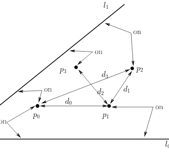
Different representations of geometric constructions in dynamic geometry have been proposed in the literature, [70, 83]. According to Kortenkamp and Denner-Broser, [16, 70], a convenient way to represent geometric constructions in dynamic geometry is Geometric Straight-Line Programs (GSP). A GSP consists of free points and dependent elements like a line through two points, the point where two lines intersect or the bisector of a segment. A GSP can be seen as a sequence of construction steps such that once values have been assigned to the free points, generates an actual construction that places free and dependent elements with respect to each others. Figure 2.10, shows a GSP and an actual construction, [15, 16].
The most important problem dynamic geometry must face is derived from ambiguities. Many constructions have not a unique solution (think for example in the intersection of a line and a circle), and to decide which one is the correct one, or at least the one the user is expecting to see, is not a simple question. Some characteristics, which we now explain, have been stated to define the behavior of the systems with respect to ambiguity, see for example [70].
2.4 Dynamic geometry 25
motion of the dependent elements. Determinism assures that, when passing through a point of multiple solutions, the system will always show the same one.
Conservatismin a dynamic geometry system guarantees that the final position of the dependent objects are the same for the same final position of the free objects, regardless of the path followed by them. That means that the final solution instance is independent from the path followed to reach it.
Finally, continuity is the property by which the movements of the dependent objects are continuous for continuous movements of the free elements. Continuity assures that no undesired “jumps” occur in the position of the geometric objects in the construction, and is a very desirable property, since users are expecting to see always a continuous behavior. Many works state that continuity and determinism are mutually exclusive, [16, 70, 83]. We will elaborate on this point in Chapter 6.
The main difference arising between geometric constraint solving and dynamic geometry is that, in dynamic geometry, the user is in charge of actually defining step by step the construction process that eventually will lead to the solution of the problem under study.
Setting up a problem in geometric constraint solving entails the geometric sketching of the problem by means of a user interface in which the set of geometric objects and relations among them are established. The solver analyzes then the problem, yielding the construction plan to solve it, if possible. Finally, a solution instance is shown on the screen, and the user is able to test the behavior of the construction by changing the specific parameter assignment given to the variant parameter.
Setting up a problem in dynamic geometry also entails the geometric modeling of the problem by means of a user interface, but the construction plan is actually given by the user when sketching the problem. Therefore a dynamic geometry system usefulness is basically limited by the user’s abilities. The solution instance is shown on the screen, and the user is able to generate the motion of the whole construction by dragging a free geometric object in the model.
Table 2.2 summarizes the different actions necessary to set up a problem in geometric constraint solving and in dynamic geometry systems, specifying the actor of each action.
2.4.2 Constraint-based dynamic geometry
26 Preliminaries
Actor
Action Dynamic geometry Geometric constraint
Geometric modeling user user
Construction plan user system
Testing user system/user
Table 2.2: Actions necessary to set up a problem, and their actors.
Although traditionally static, geometric constraint problems represent suitably dynamic geometry behaviors when we let a degree of freedom to move the system. In this way, dy-namic geometry can be parameterized by the degree of freedom of the geometric constraint problem.
As pointed out above, the main drawback of dynamic geometry with respect to geo-metric constraint solving is the necessity of the intervention of the user in the construction of any geometric instance. Geometric constraint solving skips this problem thanks to the solver, which computes the placement of each geometric object observing the constraints among them.
We call constraint-based dynamic geometry to the inclusion of a constructive geometric constraint solver into a dynamic geometry system. Thanks to the constructive solver, constraint-based dynamic geometry is able to construct a solution instance without the need of the user, settling the problem above. Moreover, for any value given to the variant parameter, the system is able to compute the solution instance following the construction plan yield by the solver, and show the result in real time.
Setting up a problem in constraint-based dynamic geometry entails the geometric sketching of the problem by means of the dynamic geometry system user interface, speci-fying geometric objects and relations among them. The solver analyzes then the problem, yielding the construction plan to solve it, if possible. Finally, a solution instance is shown on the screen, and the user is able to test the behavior of the construction by changing the specific parameter assignment given to the variant parameter.
In [25], Freixaset al. reported on a Constraint-Based dynamic geometry System based on constructive geometric constraint solving. In this technology, the user defines a geomet-ric problem by sketching some geometgeomet-ric elements taken from a given repertoire (points, lines, circles, etc) and annotates the sketch with a set of geometric relationships (point-point distance, point-line distance, angle between two lines and so on) that must be fulfilled.