Remittances and life cycle deficits in Latin America

www.depeco.econo.unlp.edu.ar/cedlas

C

C

|

E

_E

|

D

_D

|

L

_L

|

A

_A

|

S

_S

Centro de Estudios

Distributivos, Laborales y Sociales

Maestría en Economía Universidad Nacional de La Plata

Remittances and Life Cycle Deficits in Latin

America

Ricardo Bebczuk y Diego Battistón

August 29, 2009 Final Version

World Bank

Remittances and Life Cycle Deficits in Latin America

Ricardo Bebczuk and Diego Battistón

CEDLAS-UNLP

Abstract

The paper investigates the effect of remittances on the coverage of financial deficits arising during youth and retirement years and their influence on some household behaviors. To this end, household survey information is used from Ecuador, Honduras, Mexico and Nicaragua to perform a number of econometric tests exploring the linkage between remittances and a battery of health, education and work outcomes dealing with young and elderly household members. The main overall finding is that, with variations across countries and regression specifications, remittances generally appear to exert a positive and robust impact. In particular, with few exceptions, remittances (a) respond to the lack of pensions and especially to overall household financial deficits; (b) encourage co-residence of the elderly with younger relatives; (c) facilitate elderly’s retirement; (d) increase household expenditures in health and education; (e) foster public and private school attendance, inhibits child labor, and improve anthropometric measures.

Introduction

The objective of this paper is to investigate the role that remittances may play in financing the gap between expenditure and income arising at early and late stages of the life cycle, and in shaping living arrangements in recipient households.

Consumption theory posits that utility-maximizing agents strive for a smooth pattern of consumption over their lives, while their labor income follows a different dynamics. Specifically, labor earnings are typically nil for children as well as for older and retired workers, implying that they deal with a deficit between desired consumption and actual income. The situation is unlikely to change if they work, as these individuals are less productive than other adults, or are forced to take informal and badly paid jobs. Conversely, working adults are expected to have a surplus of labor income over expenditures, which will be used to finance consumption during retirement years.

Graphs 1 through 4 illustrate for remittances-recipient household that this popular model reassuringly fits household-level data in the countries we will subsequently study: Ecuador, Honduras, Mexico, and Nicaragua.1 The graphs also display per capita remittances added to labor income. Since we do not have any information on how remittances are allocated among household members, it is hard to pinpoint their precise impact on life cycle deficits. But assuming that remittances are shared proportionately among all family members, as done in Graphs 1-4, it can be observed that remittances cover, for the average household, a significant part of the financial gap of young and old individuals. We further discuss these life cycle deficits in Section 2.4.

1

The calculations involve a thorough analysis and decomposition of labor income and each consumption item by age following the National Transfer Accounts methodology. For details, see

Graph 1

Ecuador: Income and Consumption over the Life Cycle

Remittances-recipient households Smoothed values

0

0 4 8 ₁2 ₁6 ₂0 ₂4 ₂8 ₃2 ₃6 ₄0 ₄4 ₄8 ₅2 ₅6 ₆0 ₆4 ₆8 ₇2 ₇6 ₈0

Age

In

U

S

$

Consumption Labor income Labor income plus remittances

Graph 2

Honduras: Income and Consumption over the Life Cycle

Remittances-recipient households Smoothed values

0 1000 2000 3000 4000

0 4 8 ₁2 ₁6 ₂0 ₂4 ₂8 ₃2 ₃6 ₄0 ₄4 ₄8 ₅2 ₅6 ₆0 ₆4 ₆8 ₇2 ₇6 ₈0

Age

In

le

m

p

ir

a

s

Graph 3

Mexico: Income and Consumption over the Life Cycle

Remittances-recipient households Smoothed values

0 1000 2000 3000

0 4 8 ₁2 ₁6 ₂0 ₂4 ₂8 ₃2 ₃6 ₄0 ₄4 ₄8 ₅2 ₅6 ₆0 ₆4 ₆8 ₇2 ₇6 ₈0

Age

In

p

e

so

s

Consumption Labor income Labor income plus remittances

Graph 4

Nicaragua: Income and Consumption over the Life Cycle

Remittances-recipient households Smoothed values

0 1000 2000

0 4 8 ₁2 ₁6 ₂0 ₂4 ₂8 ₃2 ₃6 ₄0 ₄4 ₄8 ₅2 ₅6 ₆0 ₆4 ₆8 ₇2 ₇6 ₈0

Age

In

p

e

s

o

s

Our driving question is whether remittances contribute to cover the financial needs of the young and the elderly by spurring basic educational, labor, and health goals. A potential side effect of remittances that we will also investigate is whether they set off changes in living arrangements. To this end, we will work with the latest available national, multi-purpose household surveys conducted in Ecuador (2006), Honduras (2004), Mexico (2006), and Nicaragua (2005). These countries were chosen because, among other LAC candidates, they all are major remittances recipients and also have household-level consumption data, which constitutes a valuable input for our work.

Specifically, our plan is to produce evidence on the following story. Migrants are more likely to send remittances home if they come from households with elderly members who do not receive pensions. In reaction to this income support, the elderly stay at the migrant’s home to take care of their grandchildren. Co-residence, in turn, has consequences on the well-being of both old and young household members. The elderly become less likely to participate in the labor force, as they now work at home, and may also have more means to cover for their typically high health expenses. As for the children, in particular those old enough to work (say, those aged 11-17), the presence of the elderly frees them from the need to drop out from school to babysit their younger siblings. In addition to these effects, we will examine whether remittances relax life cycle financial deficits by giving rise to: (a) Easier access to private schooling and higher education expenses; (b) Less child labor; and (c) Better anthropometric measures among children.

Orozco (2009)). Moreover, this will mean that about 1 million households throughout the region will stop receiving remittances this year and another 4 million households will see their remittances cut by 10%.

Section 1: Data

In this section we will provide a first approximation to the relationship between remittances and several outcomes concerning the youth and the elderly. Data for each of the four countries will be presented, splitting the sample into recipient and non-recipient households along with the statistical significance of the difference. The resulting statistics will hint some clues as to whether families are likely to receive remittances to alleviate financial deficits in the early and late stages of life.2These links will be examined more thoroughly later on by applying multivariate econometric techniques.

Table 1 depicts the connection of remittances with income and poverty patterns. First to notice is the fact that the percentage of households with remittances is not high, ranging from 5.7% in Mexico to 20.4% in Nicaragua, with intermediate values for Ecuador and Honduras (16.2%). But still remittances constitute an important addition to the recipient households’ income, representing 15.5% in Ecuador, 19% in Nicaragua, 30.6% in Honduras and 49.3% in Mexico.3 This incidence is exacerbated in the case of poor households in Ecuador (57.7% of total income), Honduras (79.9%) and Mexico (80.4%). While these values largely exceed those for non-poor households in these countries, the wedge between poor and non-poor is rather narrow in Nicaragua (23.0% versus 18.7%). In terms of per capita income, remittances explain a pronounced increase of between 18.4% in Ecuador to 97.2% in Mexico. The fraction of poor families (measured by the US$2 poverty line) is much lower among recipient vis-à-vis non-recipient households in Ecuador (difference of 5.7 percentage points based on before-remittances income figures), Honduras (8.8) and Nicaragua (17.2).4The exception is Mexico, where 46.5% of recipient households and 12.4% of non-recipient ones are poor according to pre-remittances income. As in the other countries, pre-remittances to Mexico drastically diminish

2

Our observations coincide to the most part with the evidence collected for various Latin American countries, including those here studied, by Acosta, Fajnzylber and Lopez (2007).

3

It must be noted of course that the difference between post- and pre-remittances income is magnified by the fact that the latter is affected by the lost income of the member/s leaving for a foreign country. We calculate and use the counterfactual income later on in Section 2.

4

poverty among recipient households, which goes down to 10% from the above figure of 46.5%.

Given our interest in the use of remittances to finance consumption during retirement, (which would imply some substitution between pensions and remittances), we present Tables 2 and 3 to shed some preliminary light on the subject. These tables confirm that formal old-age income support is thin in both the extent of elderly population coverage and the size of pensions, reinforcing the potential income-compensating role of remittances. To begin, Table 2 shows that a majority of households with elderly members have neither pensions nor remittances: 57.6% in Ecuador, 74.5% in Honduras, 61.2% in Mexico and 53.0% in Nicaragua. Offering some initial backing to the offsetting role of remittances in retirement years, they appear to be more prevalent among families without pensions than otherwise. For instance, 14.6% of all Ecuadorian households with no pensions have remittances, but just 7.6% have both of them. The same figures for Honduras, Mexico and Nicaragua are 16.1% and 3.2%, 7.2% and 1.2%, and 30.9% and 7.5%, respectively. A similar conclusion emerges from the proportion of income explained by remittances in pension recipient and non-recipient families, which amount to 9.8% and 18.3%, respectively in Ecuador, 21.8% and 25.4% in Honduras, 27.5% and 36.6% in Mexico, and 15.8% and 18.6% in Nicaragua.5

Table 4 compares basic features of recipient and non-recipient households. The household size, number of children and number of elderly are not visibly different between these two groups. Recipient households, though, are more likely to have an elderly member, which is probably related to the need to take care of children after the departure of either of their parents. Households are headed by women or elderly members much more frequently in recipients than in non-recipients, but still this fraction is not as high as might be expected. Specifically, the data teaches us that the head in recipient households is an adult male under 65 –that is, the kind of individual a priori most likely

5

to migrate- in 49% of the cases in Ecuador, 39.7% in Honduras, 19.4% in Mexico and 21.2% in Nicaragua. In a related vein, in only 29.1% of the recipient households in Ecuador the migrant was the former head, and in just 27.6% of Honduran recipient families the current head is the migrant’s spouse. Recipient families are predominantly urban vis-à-vis non-recipient ones, again with the exception of Mexico. The years of education of the head in recipient households is slightly larger than in non-recipients, save for Mexico (5.4 years against 8.0 in non-recipients), but a noteworthy feature is that migrant’s education is between 2 and 4 years longer than that attained by the household head at home (unfortunately, migrant data is not available for Mexico).

Table 5 summarizes the selected outcomes for children and older members in recipient and non-recipient households. A quick inspection of the data delivers a disheartening general landscape in terms of human capital investments during the childhood and of old-age wellbeing in these countries, yet slightly mitigated in some remittances-recipient households. Regarding the elderly, statistically significant differences in favor of the latter households vis-à-vis non-recipient are observed for: (i) Percentage of individuals not invoking economic reasons for not visiting a doctor when ill in Ecuador; (ii) Regular medical checkups in Honduras; (iii) No labor participation in Nicaragua; (iv) Early retirement (proportion of people aged 55-70 already retired) in all four countries; and (v) Fraction of elderly living alone or with other elderly in Ecuador, Honduras and Nicaragua, where less, rather than more, older people from recipient households has a house of their own. This last difference reveals that housing decisions depend not just upon budget constraints but also upon intra-household arrangements. For instance, older people may have the means to leave, but they may rather stay to take care of the children while the parents are out working.

Section 2: Results

2.1 Methodological issues

Before going into the estimations, it is necessary to discuss three serious methodological issues that are paramount to a meaningful interpretation of our findings, namely, (1) The transmission channel from remittances to life cycle deficits, in particular the relationship between individual- and household-level deficits, and (2) The potential endogeneity of remittances.

A proper analysis of the transmission channel also requires a clear identification of the outcomes that remittances are able to affect. Although households may target a broad array of goals for their members, we would be able to claim a positive effect of remittances on overcoming financial deficits only if we focus on goals that involve pecuniary costs. For example, a complete vaccination plan for children or attendance to public school may be available at no cost from government providers, so remittances are inconsequential in this case.6 On the other hand, failure to reach normal anthropometric measures or the existence of child labor directly attest to the insufficiency of regular household income to cover basic necessities, and money from remittances might be instrumental in solving this deficiency.7

In a related vein, another factor to take into account is that financial deficits are bound to come up in people lacking enough earnings to afford current expenses, but this does not imply that the household as a whole is in deficit. For example, it is clear that a high income household can easily fill the financing gaps of its young and old members, just by making use of the surpluses generated by the working members, and without any need for additional resources in the form of credit or remittances. Conversely, whenever pre-remittances household income is insufficient to adequately provide for the needs of children and old members, it is likely that some basic expenses for health and education purposes may be cut, that children may start early their working career and that old members may continue theirs beyond a typical retirement age. The empirical relevance of this argument can be tested by interacting remittances with a variable reflecting the household financial constraint, that is, the gap between actual household income and the minimum needed to reach the desirable outcomes for their young and old members. As

6

By the same token, we must assume that households have a strong preference for these costly services over free-of-charge public substitutes and that there exist no non-economic reasons for refraining to use private services (for example, parents may feel intimidated to send their children to private schools in light of social differences).

7

this gap is not observable, we will take poverty as a proxy for financial constraints.8We use the 2 dollar poverty line based on household income before remittances.9

Turning now to the other major methodological caveat, a serious pitfall at the moment of interpreting OLS results is that estimates may be contaminated by endogeneity bias. Whenever endogeneity is present, one may tend to mistakenly attach to remittances a welfare-improving effect that they do not have. Endogeneity emerges as a consequence of omitting a relevant variable in the model affecting simultaneously remittances and the dependent variable. The underlying misspecification stems from selection bias, meaning that the set of remittances senders is not randomly chosen but self-selects on the basis of observable and non-observable characteristics that are not nested into the econometric model and that also have an impact on the outcome under study. When these characteristics are observable, the obvious solution is to include this variable on the right-hand side. When they are not observable, one must follow an instrumental variable (IV) technique, aimed to identifying one or more variables that are highly correlated to the endogenous explanatory variable (that is, remittances) but not directly associated to the dependent variable.

Economic theory is called for in guiding the search for endogeneity bias in a regression. The education/remittances nexus may be plagued with selection bias caused by the omission of household wealth and income shocks in the estimated equations. In the presence of high migration costs and financial constraints, individuals from wealthier households may be more likely to migrate (and send money to the relatives left behind). At the same time, these families are expected to place a higher value on education and to

8

This might be an over-conservative choice as long as some strictly non-poor families might as well be unable to afford some expenses from our list of desirable outcomes, but it still is a safe choice in view of the lack of a more precise measure of financial constraint.

9

have healthier children, all of which heightens the probability of regularly attending school. In turn, a volatile domestic income may simultaneously push adult members towards foreign labor markets and pull children out of school to take a job or stay at home babysitting her siblings while adults work outside. In the end, we may observe a positive correlation between education and remittances being explained not by a causal link but by the joint influence of a third variable.10

Labor participation is most likely to be exposed to a similar econometric qualification. A case in point is one in which an adverse economic situation forces young and/or old household members to enter the labor market at the same time that leads adults into moving abroad in search of better job opportunities.11In children health matters, extreme poverty or negative income shocks may give rise to malnutrition and deficient anthropometric measures, accompanied by the adults’ decision to migrate in order to make up for the small or lost income at home.

Despite these considerations, endogeneity needs to be tested rather than just postulated – endogeneity is possible but not certain, and the size of such bias is unknown a priori. In consequence, in order to detect this potential endogeneity and then circumvent it if necessary, we will start by controlling for household wealth. House ownership is a nice proxy for pre-remittances wealth in that the odds that a household might have bought a house out of remittances are quite slim.12For one, annual remittances are typically small relative to house prices. Secondly, and adding to the previous point, recipients consulted in different surveys inform that most of the money is channeled towards current expenses, and a marginal portion, well below 10%, goes to real state purchases.13,14

10

Ability -an unobservable variable- may play a similar role to household wealth.

11

The decision to send some adult members to work in other countries can also be based on a strategic household choice to diversify local systemic risk rather than just responding ex post to a negative shock.

12

Acosta (2006) employs an index of household assets, but one cannot be sure without further information whether some of these assets were bought with remittances money, that is, these assets might represent an endogenous outcome themselves.

13

Our preferred instrumental variable is the migrant’s social network, measured by the percentage of households from a given city living abroad (see Acosta (2006)). By reducing the cost of migrating and improving the labor prospects of a new migrant, the presence of relatives or neighbors in a foreign community increases the probability of sending remittances, without affecting any of our dependent variables, thus meeting the required conditions of a good instrument.15

2.2. Econometric results

In what follows we present our empirical findings. For the sake of clarity, and given the numerous regressions being reported, we will only comment here on the estimates on our variables of interest, leaving outside the discussion about the controlling set of socio-demographic variables included in each case, which generally yield the expected sign.16

Before starting, let us recall that the empirical story presented at the outset implies the verifiable hypotheses that remittances: (a) are more likely to be sent to households with elderly lacking pension payments; (b) make it more likely the co-residence of the elderly with younger relatives, in particular in households with children that need to be taken care of; (c) facilitate the retirement of older workers at the legal retirement age or even earlier than that, in response to their new role at home; (d) help the elderly afford their

14

A sensible reply to this statement is that money is fungible, and one cannot take the reported remittances allocation as a reliable data on how money is spent. For example, it would be possible that remittances allow recipients to save most of their regular income for house purchase purposes, in which case remittances may be indirectly financing the purchase of a house. Unfortunately, surveys do not usually provide information on the substitution between remittances and other sources of income, but an educated guess dictates that survey respondents refer to the overall allocation of household income - the very fungibility property would make it difficult for the recipients themselves to isolate the use of each type of income.

15

McKenzie and Sasin (2007) contend that village network are not always such a good instrument for outcomes abroad, citing the case in which the village network are an artifact to get better jobs and boost migrant’s earnings.

16

usually steep health expenditures; and (e) foster children school attendance by liberating them from the obligation of babysitting younger siblings while parents are at work.

the deficit of the older members –as an illustration, if the elderly receives no pension but her family makes a good income, the relative living abroad may not feel inclined to make any transfer. On empirical grounds, however, the transformed pension variable yields estimates that do not differ much from those of the pension dummy alone.

One may legitimately wonder why the altruistic model, under which migrants support old-age consumption, seems to apply to Ecuador and Mexico but not to Honduras and Nicaragua. Unfortunately, lack of more detailed information prevents us from inferring the strategic decisions of the household and the migrant. For a variety of reasons, migrants may not be especially concerned about the older members of the family, targeting instead their financial assistance towards items favoring exclusively younger members or the household as a whole (for example, the purchase of durable goods or the payment of the rent). In this spirit, the same Table 6 shows that the number of children under 15 years old increases the likelihood of receiving remittances in all countries but Nicaragua. It is also possible that the migrant pursues some personal, non-altruistic goals, such as building up a stock of wealth for future use upon returning home.17The drawback of this argument is that, under this hypothesis, the migrant would not be looking after her family, and hence the remittances reception model would yield non-significant estimates on most household characteristics. Since Table 6 proves otherwise, the explanation for cross-country differences should be looked for elsewhere -provided information permits, which unfortunately is not the case in the context of our household surveys.

Moving on, Table 7 displays the determinants of the probability of co-residence of older individuals (aged 65+) and children (aged 10 or below) in the same household. The remittances dummy bears a positive and significant sign (with marginal probabilities ranging from 6% to 14%) in all countries but Nicaragua, where the estimate is significantly negative. However, when we interact this variable with the poverty dummy already used in Table 6, all four coefficients turn positive and significant, the most likely reason being that poor families have more incentives to exploit economies of scale by

17

avoiding the extra expenditure of the elderly paying rent or buying a house for leaving by themselves.

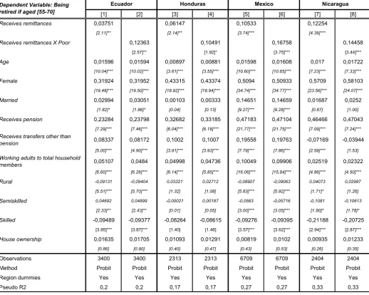
As stated at the beginning, we expect the elderly (65+ years old) from recipient households to self-exclude from the labor market. This is exactly what we find in Table 8 in all countries, but only with statistical significance in Mexico and Nicaragua. Nevertheless, the result becomes highly significant once we interact the remittances reception variable with poverty, which might explained by the fact that in poor families it is likely that all adult members, included women, work outside, making it more imperative the presence of the elderly to look after the children. The same storyline justifies the evidence of early retirement among individuals 55-70 years old encountered in Table 9, where the effect is present with both the remittances dummy and, with a larger point estimate, with the remittances-poverty interaction.18

The impact of remittances on health expenditures is estimated in Table 10. In this case, we test four different remittances-based variables: besides the remittances dummy and the same binary variable interacted with poverty, we evaluate the effect of the logarithm of per capita remittances and the latter again interacted with poverty –the value of remittances may be of interest because the dependent variable is a monetary variable. Notice that the sample size is substantially smaller when the value of remittances, as opposed to the dummy variable, is employed -in some cases, the remittances value sample is less than one tenth the dummy sample. This provides an unintended but useful robustness check for our results. Table 10 reveals that remittances also seem to boost health expenditures in all countries but Honduras.19,20Per capita remittances is significant in all three countries, while the other remittances variables are significant in some countries but not in others. Finally, the claimed positive effect on school attendance

18

We extend the early retirement effect until 70 years old because it is not unusual in our country sample for people to work beyond the legal retirement age.

19

Although this item comprises expenses benefiting other household members, it is natural to think that older individuals have a larger and more frequent demand for health services. In any case, we replied the exercise using the imputed health expenditures to the elderly members, resorting to the National Transfer Accounts (NTA) methodology, without observing any worth mentioning change in the overall results.

20

among children between 11 and 17 years old is confirmed in Table 11.21 Mexico is the only exception. This situation might stem from the fact that Mexican migrants come from households with low levels of education, as shown earlier, and thus remittances might not modify the seemingly low value placed on human capital accumulation.

Leaving behind the nexus between remittances and co-residence and its impact on some household expenses and decisions, we now turn to additional outcomes likely to be influenced by remittances. Access to private school, according to Table 12, is once again enhanced in recipient households in all countries; the interaction between the remittances dummy and poverty is always significant, while per capita remittances is significant in all countries but Mexico. Based on Table 13, in all countries the reception of remittances and their size spur this consumption item (yet though some negative signs are found for poor families in Nicaragua and Honduras). Table 14 shows that child labor lowers in recipient households in all four countries, and this effect is uniformly significant for the remittances dummy (and for some, but not all, of the other three remittances variables). Finally, Tables 15 and 16 explain, for Ecuador and Honduras, the determinants of two anthropometric measures: the height-to-age and the weight-to-age z-scores. Results point to a positive effect for both children health indicators in Honduras and, with borderline statistical significance, also in Ecuador.

Having reported the main evidence, it may be helpful to visualize the overall results in summary Table 17. Along with the expected sign for each dependent variable, the table contains the cases where at least one of the remittances variables had the correct sign and was significant at 10% or less (labeled as Y, for Yes), the cases where none of such variables met these conditions (labeled as N, for No), and those with significant yet conflicting results (denoted by an interrogation mark). Based on this classification, we find that our empirical predictions mostly tend to be confirmed by the data. Out of a total 40 cells (11 dependent variables times 4 countries, minus 4 cases without data), only 4

21

contradict the priors and another two deliver mixed results. Looking closer to these cases, we have (i) the lack of response of remittances to pensions in Honduras and Nicaragua, which might have to do either with a different household behavioral model or with the fact that the number of pensioners is too small in these countries and the statistical tests are in consequence not fully reliable; (ii) the level of health expenditures in Honduras; and (iii) co-residence in Nicaragua; and (iv) School attendance and education expenditures in Mexico, where the educational background of the recipient household might be at play in rationalizing the results. As argued before, further information on the migrant and his or her household of original may come in handy to further inquiry on this subject.

2.3 Dealing with potential endogeneity

Before closing, attention must be paid to the endogeneity bias that might potentially distort our results by inflating the coefficients and attaching a spurious causal effect to remittances. The social network variable previously introduced was employed to instrument remittances. This variable is proxied by the number of migrants from the same village as the household, as a percentage of total village population.22 As can be seen there, most estimates become non-significant after implementing this instrumental variable method. However, we are not fully convinced about the instrument’s suitability in our case. In the first place, the first-stage equations regressing the remittances variables on the social network variable and other exogenous variables do not have a compellingly high goodness-of-fit. Secondly, the IV coefficients were dramatically different in both size and sign from the probit and OLS estimates presented in Section 2.2, casting serious doubt as to the quality of this instrument. In view of this, we opt for not reporting the results.

Instead, we have made use of propensity matching score to circumvent the risk of any endogeneity contaminating previous estimations. In a nutshell, this non-parametric

22

technique searches for households with similar features in crucial observable aspects, but differ in terms of a certain treatment (in our case, receiving remittances or not). These similarities include the level of counterfactual income, that is, we impute to recipient households an estimation of the lost migrant’s income. By comparing household without observable differences, we are minimizing the omitted variable problem, thus to a great deal getting rid of the source of any possible endogeneity. The methodological details of the calculation of the counterfactual income and the estimation of propensity matching scores are relegated to an Annex at the end of the document.

The results appear in Table 18 (elderly-related outcomes) and 19 (child-related outcomes), and are by and large in line with our previous findings, providing reassuring support for our empirical claims.

2.4 An alternative approach

Our testing approach so far was centered on looking at how some household characteristics and outcomes affect and are affected by remittances. Since we are interested in the link between remittances and life cycle deficits, an appealing and complementary procedure consists of examining these variables more directly. To this end, we computed the ratio [Consumption - Labor Income]/Consumption for household members aged 14 and under, those aged 65 and above, and for the whole household. Expenditure and income by age was measured through the National Transfer Account method already employed in Section 1. This ratio is positive (with a maximum of 1 when labor income is zero) for individuals confronting a deficit of own labor income vis-à-vis consumption, and gets negative (with a maximum absolute value equal to Labor Income/Consumption) for surplus individuals.

lower surpluses).23 This puts on the table fresh evidence on the positive role of remittances on smoothing household expenditure.

Less clear is whether remittances react more strongly to life cycle or household deficits. Rephrasing, we wonder whether migrants feel more compelled to sending money back home if they identify deficits among the more vulnerable age groups in the household (young and old members), or instead they worry about the deficit of the household as a whole. The latter case would not imply that they do not care about the fortune of children and elderly relatives, but that they look more broadly into the household’s financial troubles, in the sense we already argue in Section 2.1. To shed some light on this issue, we run some regressions reproduced in Table 21, where the dependent variable is the reception of remittances and the explanatory variables are the combined deficit of the members under 15 and above 64 years old and the whole household’s deficit. Additional key controls are also included. The main conclusion is that household deficits seem to be more relevant than life cycle deficits: for one, when entered separately, the estimated coefficient on the combined life cycle deficit is either non-significant (as in Mexico) or much lower, by as much as three times, than the household deficit coefficient; second, and foremost, when both deficits are included, only the latter remains positive and highly significant.

23

Conclusions

Exploiting recent national household surveys from Ecuador, Honduras, Mexico and Nicaragua, our paper aimed to seek empirical evidence on the hypothesis that remittances serve the goal, among others, of covering financial deficits arising in the early and late stages of life. Under this hypothesis, households receiving remittances should be able to finance key expenditures in human capital and health, as well as avoiding labor participation for young and old household members. Standard descriptive statistics and multivariate regression exercises lend broad support to the assertion to remittances seem to exert a positive role. In particular, with few exceptions, remittances (a) respond to the lack of pensions and especially to overall household financial deficits; (b) encourage co-residence of elderly with younger relatives; (c) facilitate labor retirement at legal or early ages; (d) increase household expenditures in health and education; (e) foster public and private school attendance, inhibits child labor, and improve anthropometric measures.

References

Acosta P., P. Fajnzylber and H. Lopez (2007a), “Remittances and Household Behavior: Evidence for Latin America”, in Fajnzylber P. and H. Lopez (eds.), Remittances and Development: Lessons from Latin America, World Bank.

Acosta P., P. Fajnzylber and H. Lopez (2007b), “How Important are Remittances in Latin America?”, in Fajnzylber P. and H. Lopez (eds.), Remittances and Development: Lessons from Latin America, World Bank.

Acosta P., P. Fajnzylber and H. Lopez (2007c), “The Impact of Remittances on Poverty and Human Capital: Evidence from Latin American Household Surveys”, in Özden Ç. and M. Schiff (eds.), International Migration, Economic Development and Policy, World Bank-Palgrave Macmillan.

Acosta P. (2006), “Labor Supply, School Attendance, and Remittances from International Migration: The Case of El Salvador”, Policy Research Working Paper No. 3903, World Bank, April.

Adams R. (2005), “Remittances, Household Expenditures and Investment in Guatemala”, Policy Research Working Paper No. 3532, World Bank, March.

Amuedo-Dorantes C. and S. Pozo (2006), “Migration, Remittances, and Male and Female Employment Patterns”, American Economic Review, Vol. 96, No. 2.

Antman F. (2008), “Who Cares for the Elderly? Intrafamily Resource Allocation and Migration in Mexico”, mimeo, University of Colorado at Boulder, June.

Banks J., R. Blundell and A. Lewbel (1997), “Quadratic Engel Curves and Consumer Demand”, Review of Economics and Statistics, Vol. 79, No.4.

BCH (2008), “Remesas familiares: Informe de Encuesta”, Banco Central de Honduras, January.

Becker S. and Ichinos A. (2002) , Estimation of average treatment effects based on propensity scores , Stata Journal, 2002, vol. 2, issue 4, pages 358-377.

CESOP (2004), “El impacto de las remesas familiares en México y su uso productivo”, mimeo, Centro de Estudios Sociales y de Opinión Pública, December.

Görlich D., T. Mahmoud and C. Trebesch (2007), “Explaining Labor Market Inactivity in Migrant-Sending Families: Housework, Hammock, or Higher Education?”, Kiel Working Paper No. 391, December, Kiel Institute.

Hagen-Zanker J. and M. Siegel (2007), “The determinants of remittances: A review of the literature”, Working Paper No. 3, Maastricht Graduate School of Governance.

Huenchuan S. and J. Guzmán (2006), “Seguridad económica y pobreza en la vejez: tensiones, expresiones y desafíos para el diseño de políticas”, Notas de Población No. 83, ECLAC.

IOM (2007), “Encuesta sobre remesas 2007: Perspectiva de género”, Cuadernos de Trabajo sobre Migración, International Organization for Migration, September.

Mansuri G. (2007), “Does Work Migration Spur Investment in Origin Communities? Entrepreneurship, Schooling, and Child Health in Rural Pakistan”, in Özden Ç. and M. Schiff (eds.), International Migration, Economic Development and Policy, World Bank-Palgrave Macmillan.

McKenzie D. and M. Sasin (2007), “Migration, Remittances, Poverty, and Human Capital: Conceptual and empirical challenges”, World Bank Policy Research Working Paper No. 4272, July.

Orozco (2009), “Migration and remittances in times of recession: Effects on Latin American and Caribbean Economies”, Document No. 5/09, Latin American and Caribbean Economic System, May.

Pfau W. and G. Long (2009), “Remittances, Living Arrangements, and the Welfare of the Elderly in Vietnam”, Working Paper 0901, Vietnam Development Forum, March.

Rodriguez E. and E. Tiongson (2001), “Temporary Migration Overseas and Household Labor Supply: Evidence from Urban Philippines”, International Migration Review, Vol. 35, No. 3.

Rosenbaum P. and D. Rubin (1983), “The Central Role of the Propensity Score in Observational Studies for Causal Effects”, Biometrica, Vol. 70 (1), 41-55.

Rosenbaum P. and D. Rubin (1984), “Reducing Bias in Observational Studies using Subclassification on the Propensity Score”, Journal of the American Statistical Association 79, 516-524.

Methodological Annex for Section 2.3

We have followed the methodology advanced by Acosta, Calderon and Fajnzylber (2008), who use a two step selection model for estimate the counterfactual “non remittances income”. The reduced-form income equation for the household adopts the following specification:

i 2 2 2

log(Y )  X_i H_i_i

where Yi is the per capita non-remittances income, Xi is a vector of household

characteristics , Hi is a set of characteristics of the household head, and i is unobserved heterogeneity in the income generation. As we have mentioned, the income “net of remittances” is a bad proxy for Yi, so we can assume that Yi is only observed for a

subsample (the non recipient households) and use this for predicting the non remittances income of the rest of the sample (the recipient households). Running OLS on the former equation would lead to inconsistent estimates of the parameters (and hence inconsistent predictions) because as we have shown in previous sections, there exists evidence suggesting that migrants are not randomly selected from the pool of households. Acosta, Calderon and Fajnzylber (2008) propose to use a two step model based on Heckman (1979) framework, including in the income equation a variable that reflects the “propensity to receive remittances” (or to migrate). The two equations of the model have the following specification:

*

1 1 1

i 2 2 2

selection equation

income equation

log(Y )

i i i i i

i i i i

M X H Z

X H

    

    

    

    

where Ziare a set of variables related with the decision of migration/sending remittances

but not related with the income generation (the exclusion restriction). The variable













i X H Z X H Z

            is the inverse Mill’s ratio, with

1 1

( | )

i E vi i Xi Hi Zi

       and  cov( ,v_i _i) / var( )_i . M*i is the (unobserved)

propensity to not receives remittances, and we only observe Yifor the subsample with M*

>0.

After estimating the income equation for the non-recipient household subsample, we can consistently predict the non-remittance income for the recipient households24. Note that the set of variables Xi used for prediction must be based on the pre-migration scenario, so

we have to “correct” some variables using the migrant information. This is for example the case of the household size, where we have used the observed size plus the number of migrants. The variables included in Ziare the migrant networks, an index of assets of the

house and their interaction. The variables included in the Xiand Hi set are the size of the

household, the number of members in different age and gender groups, the mean and the maximum years of education of the household, the age of the head and its squared.

24

Finally, we add to the income prediction of the model an error component generated from a distribution with the same properties (mean and variance) than the distribution of errors of the estimated equation.

Once we have constructed the counterfactual income for the scenario with no migration and no remittances, we still have to deal with the selection problem caused by the fact that migrants are not randomly selected from the pool of all household in the sample. There are several ways to correct this bias, but we can take advantage of the binary nature of our interest variable (remittances reception) and apply the instrumental of the evaluation literature. For allowing some parallelism with the evaluation literature notation, we define the remittances reception as the “treatment variable”. Suppose that we are interested in the effect of remittances on a particular outcome Y and it can take two different values depending of the treatment status. We call YiT the outcome resulting

when the individual i receives remittances and YiNT the outcome resulting if the same

individual don’t receive remittances. There is bias arising because we can’t observe the same individual in both scenarios. More technically, we can only observe (YiT|Di=1) and

(YiNT|Di=0) where Di is an observed dummy indicating if the individual receives

remittances. A simple mean difference of these two variables can be expressed as E[YiT|Di=1] - E[YiNT|Di=0] and correspond to the differences we can estimate from the

descriptive tables commented before. Adding and subtracting the term E[YiNT|Di=1], we

obtain:

E[YiT|Di=1] - E[YiNT|Di=1]+ E[YiNT|Di=1] -E[YiNT|Di=0] =

E[YiT - YiNT |Di=1] + E[YiNT|Di=1]-E[YiNT|Di=0]

The first term, E[YiT - YiNT |Di=1] is known as the “Average Treatment Effect on the

Treated” (ATT) and correspond to the effect of the remittances on the subsample of recipients25. The second term E[YiNT|Di=1] - E[YiNT|Di=0] is the selection bias that is

unobserved because of E[YiNT|Di=1]. Note that the bias arise from the fact that we don’t

observe the outcome that the individuals with remittances (D=1) would have had if they hadn’t received remittances. The bias tells us that the treated individuals (recipients) can have systematic differences in the output independent of the treatment status. If the treatment status is completely random we don’t expect systematic differences between treated and not treated and the bias should tend to zero. A natural solution for correcting this bias is the comparison between treated and not treated individuals but only those with similar characteristics, arguing in this case that the only differences in outcomes come from the treatment status (the remittance reception)26. Every individual i should be compared (matched) with a “similar” group of individuals called the “control group for individual i”. This solution is not possible (neither practical) when the differences between individuals are due to several variables. Rosenbaum and Rubin (1983) proved that if the exposure to treatment is random given the observed characteristics (they assumes that there are not selection in unobservables), it is also random for similar values of the one-dimensional variable p(X) = Pr(D=1|X)=E(D|X), where X is a set of

25

The average treatment effect on the full sample requires additional techniques and assumptions

26

treatment27observed characteristics and p(X) is the “propensity score” (PS) and it can be estimated using any standard probability model like probit or logit. This strong result implies that we can construct a control group for every treated individual using non treated individuals with similar propensity score instead of making multidimensional matching. Formally, the assumption needed to perform the propensity score matching is that ( T, NT) /

Y Y D X , in other words, once we have conditioned on X, the effect of receiving remittances must be the same either the individuals are actually treated or not28. This assumption prevents the selection in unobserved characteristics and is a strong assumption in our analysis. The variables we used to perform the propensity score estimation are the same used in the previous OLS and Probit regressions corresponding to the respective outcome of interest.

Once we have estimated the PS, there are different methods to construct the “control group” of every treated individual using the subsample of non treated individuals and measure the Average Treatment Effect on Treated29. The most popular way is to use the “K-nearest neighbor matching method" and consist in comparing the outcome of every treated individual with the outcome of kindividuals among the non treated group with the closest estimated PS. Averaging over the treated individuals, we have the ATT estimation. The “Radius matching method”follows a similar idea, using as control group for the individual i the observations in the non treated set with an estimated PS such that the difference in absolute value with the PS estimated for i is less than a threshold r. The “Kernel matching method” differs from the previous because it uses the full set of non treated individuals (relying on the common support) but it weights them with different values according to the distance with the PS of the treated individual iand the weights are given by a kernel smooth function. Formally, the estimated ATT is given by:

      kernel 1 j i NT j

j NT n

T i T

i T _{k i}

k NT n

p p

Y G

h

ATT Y

N p p

G h  _               _  _     _{ }   _{ }   







Where T is the set of individuals who receives remittances (treated), NT is the set of individuals not receiving remittances, NT is the number of individuals receiving remittances, G(.)is a kernel function with a bandwith parameter hn.

There are also several matching estimators in the literature that we don’t comment here30.

27

Note here the importance of using here the counterfactual income for a scenario of no remittances and no migration instead of the income net of remittances.

28

There are some additional technical requirements that we don’t mention here. For more details see Rosenbaum and Rubin (1983).

29

We also restrict the analysis to observations relying on the “common support”, that is observation with PSM estimated lower than the maximum PSM inside the opposite (treated or non treated) group and with estimated PSM higher than the minimum PSM of the opposite group.

30

Table 1

Remittances and Household Income Profile

R NR Diff R NR Diff R NR Diff R NR Diff

Receives remittances (%) 16.2 83.8 -67.6*** 16.2 83.8 -67.6*** 5.7 94.3 -88.5*** 20.4 79.6 -59.3***

Poor (based on income before

remittances) (%) 13.4 19.1 -5.7*** 35.0 43.9 -8.8*** 46.5 12.4 34.0*** 27.0 44.2 -17.2***

Poor (based on income after

remittances) (%) 6.7 19.1 -12.4*** 14.5 43.9 -29.3*** 10.0 12.4 -2.4*** 19.0 44.2 -25.3***

Remittances (% of household

income) - All households 15.5 0.0 30.5 0.0 49.3 0.0 19.0 0.0

Remittances (% of household

income) - Poor Households 57.7 0.0 79.9 0.0 80.4 0.0 23.0 0.0

Remittances (% of household

income) - Non-Poor Households 13.7 0.0 20.9 0.0 34.5 0.0 18.7 0.0

Per capita income before

remittances 160.2 164.9 -4.7 2120.0 1374.9 745.1*** 1072.6 2589.4 -1516.8*** 1278.1 1060.2 217.9***

Per capita income after

remittances 189.6 164.9 24.7*** 3051.9 1374.9 1677.0*** 2115.6 2589.4 -473.8*** 1578.1 1060.2 517.9***

Receives pensions (%) 12.6 7.3 5.3*** 5.7 2.2 3.6*** 6.2 11.0 -4.8*** 9.7 4.0 5.7***

Pensions (% of household

income before remittances) 4.8 2.8 2.0** 1.7 2.3 -0.6 3.2 4.5 -1.3** 2.6 1.3 1.3**

Pensions (% of household

income after remittances) 4.1 2.8 1.3** 1.2 2.3 -1.1 1.6 4.5 -2.8** 2.1 1.3 0.8

Variable/Country Ecuador 2006 Honduras 2004 Mexico 2006 Nicaragua 2005

Table 2

Remittances and Household Demographic Profile

R NR Diff R NR Diff R NR Diff R NR Diff

Household size 4.1 4.0 0.1** 5.0 4.9 0 4.0 4.0 0 4.8 5.3 -0.5***

Have children 72.4 71.3 1.1 85.4 83.3 2.1* 71.5 66.3 5.2*** 73.9 82.4 -8.5***

Number of Children (0-17 years

old) 1.6 1.6 0.0 2.3 2.3 0.0 1.8 1.5 0.3*** 1.9 2.3 -0.4***

0-5 years old 0.5 0.6 -0.1*** 0.7 0.8 -0.1*** 0.6 0.5 0.1*** 0.6 0.7 -0.1***

6-12 years old 0.6 0.7 0.0 0.9 0.9 0.0 0.7 0.6 0.1*** 0.8 1.0 -0.2***

13-17 years old 0.5 0.4 0.1*** 0.7 0.6 0.1*** 0.5 0.4 0.1*** 0.6 0.7 -0.1***

Have elderly members (65+

years old) 25.5 16.9 8.6*** 21.5 16.0 5.5*** 28.5 19.2 9.3*** 34.9 18.0 17.0*** Number of Elderly (65+ years

old) 0.3 0.2 0.1*** 0.3 0.2 0.1*** 0.4 0.2 0.1*** 0.4 0.2 0.2***

Female-Headed Household 32.4 19.5 13.0*** 42.9 21.5 21.4*** 58.6 23.1 35.5*** 50.3 25.2 25.1***

Elderly-Headed Household 18.5 13.2 5.4*** 16.4 12.4 4.0*** 23.1 15.2 7.9*** 28.5 13.2 15.3***

Rural 15.2 26.2 -11.1*** 39.5 54.0 -14.5*** 48.1 21.0 27.1*** 30.6 48.1 -17.5***

Years of education, household

head 9.0 8.4 0.6*** 5.9 4.8 1.1*** 5.4 8.0 -2.6*** 5.0 4.7 0.3**

Migrant age 33.9 31.2 2.7*** 32.6 30.4 2.2*** 33.4 31.4 2.0**

Migrant gender (male=1) 48.6 48.8 -0.2 65.4 63.1 2.4 54.7 45.3 9.3***

Migrant's years of education 12.2 12.5 -0.2 7.9 7.7 0.2 9.1 7.3 1.8***

Migrant being the former

household head 29.1 6.6 22.5***

Migrant being the spouse of

current head 27.6 16.7 10.8***

Nicaragua 2005 Mexico 2006

Variable/Country Ecuador 2006 Honduras 2004

Table 3

Fraction of households with and without remittances and pensions (in %) Households with at least one member aged 65+

Ecuador With remittances Without remittances

With pensions 7.6 20.3

Without pensions 14.6 57.6

Honduras With remittances Without remittances

With pensions 3.2 6.3

Without pensions 16.1 74.5

Mexico With remittances Without remittances

With pensions 1.2 30.4

Without pensions 7.2 61.2

Nicaragua With remittances Without remittances

With pensions 7.5 8.7

Table 4

Remittances and Pensions: Fraction of Household Income (in %) Remittances (left) and pensions (right, in parenthesis)

Households with at least one member aged 65+

Ecuador With remittances Without remittances

With pensions 9.8 (24.7) 0.0 (30.0)

Without pensions 18.3 (0.0)

Honduras With remittances Without remittances

With pensions 21.8 (22.7) 0.0 (26.7)

Without pensions 25.4 (0.0)

Mexico With remittances Without remittances

With pensions 27.5 (18.7) 0.0 (31.4)

Without pensions 36.6 (0.0)

Nicaragua With remittances Without remittances

With pensions 15.8 (17.8) 0.0 (22.2)

Table 5

Remittances and Children- and Elderly-Related Outcomes

Variable / Country

Elderly-related Outcomes R NR Diff R NR Diff R NR Diff R NR Diff

Economic reason for not

seeing a doctor if ill 32.3 44.0 -11.7*** 16.8 24.1 -7.3 7.8 7.7 0.0

Regular checkups 19.7 14.8 4.9 12.3 6.5 5.8*** 4.5 3.2 1.4

Labor participation 41.1 45.5 -4.4* 37.5 42.3 -4.7 36.4 34.5 1.9 30.0 41.8 -11.9***

Retired people aged 55-70 32.0 27.0 5.0*** 48.2 42.2 6.0** 50.5 42.3 8.2*** 47.3 33.3 13.9***

People 65+ living alone or

with other elderly 22.5 32.3 -9.7*** 11.6 16.8 -5.2** 28.1 31.2 -3.1 13.3 6.1 7.2***

Health expenses to total

consumption (%) 12.9 10.6 2.3 14.2 11.4 2.7* 7.1 6.0 1.1 9.7 7.6 2.1**

Children-related Outcomes R NR Diff R NR Diff R NR Diff R NR Diff

School attendance [6,12] 98.9 97.2 1.6*** 95.8 90.1 5.7*** 98.5 97.8 0.7 86.8 81.5 5.3***

School attendance [13,17] 86.0 77.8 8.2*** 78.4 68.9 9.5*** 76.5 75.7 0.8 75.7 67.3 8.3***

Private education [6,12] 40.8 26.2 14.6*** 12.5 7.0 5.5*** 3.7 8.4 -4.6*** 15.5 9.5 5.9***

Private education [13,17] 36.7 27.7 9.0*** 21.6 12.7 8.9*** 3.6 11.8 -8.2*** 23.8 15.9 7.9***

Weight at birth (%

underweight 2,5 kg.) 10.2 7.1 3.1*

Weight for age Z-score [0-6] -0.5 -0.7 0.2*** -0.3 -0.8 0.5***

Height for age Z-score [0-6] -0.8 -1.0 0.2*** -0.6 -1.3 0.7***

Labor participation [11-17] 23.8 29.3 -5.5*** 14.6 19.7 -5.1*** 20.1 19.0 1.1 17.3 25.6 -8.3***

Education expenses to total

consumption (%) 8.6 8.0 0.6 7.0 6.1 0.9** 7.1 9.3 -2.2** 5.6 5.0 0.6** Ecuador 2006 Honduras 2004 Mexico 2006 Nicaragua 2005

Table 6

Pensions and the Probability of Receiving Remittances Marginal probabilities

[1] [2] [3] [4] [5] [6]

Age (Household Head) 0.00061 0.00004 0.00003 -0.00363 -0.0036 -0.00362

(0.47) (0.03) (0.03) (2.43)** (2.41)** (2.43)**

Age (Household Head) Squared 0.0000 0.00001 0.00001 0.00005 0.00005 0.00005

(0.25) (0.79) (0.8) (2.94)*** (2.91)*** (2.94)***

Female household head 0.13372 0.13326 0.13322 0.17135 0.17124 0.17134

(9.44)*** (9.42)*** (9.42)*** (11.10)*** (11.09)*** (11.10)***

Married household head 0.03719 0.03753 0.03754 0.06179 0.06163 0.06177

(3.17)*** (3.21)*** (3.21)*** (4.81)*** (4.79)*** (4.80)***

0.00142 0.00162 0.00163 0.00137 0.00132 0.00136

(1.48) (1.69)* (1.70)* (1.23) (1.17) (1.21)

Rural -0.03546 -0.03657 -0.03663 0.00907 0.00899 0.00907

(4.11)*** (4.24)*** (4.25)*** (0.87) (0.86) (0.87)

Log(per capita consumption) 0.05658 0.05781 0.05789 0.09375 0.0934 0.09369

(12.01)*** (12.24)*** (12.25)*** (13.23)*** (13.17)*** (13.22)***

0.01999 0.02047 0.02047 0.02022 0.02013 0.02021

(7.28)*** (7.45)*** (7.45)*** (7.47)*** (7.44)*** (7.47)***

0.0509 0.05781 0.05803 0.0199 0.01721 0.0195

(3.69)*** (4.13)*** (4.15)*** (1.26) (1.07) (1.21)

-0.04393 0.02493

(2.62)*** (0.81)

-0.04551 0.00388

(2.71)*** (0.13)

Observations 10,849 10,849 10,849 8,124 8,124 8,124

Region dummies Yes Yes Yes Yes Yes Yes

LR chi2 541.5 548.3 548.6 569.5 569.3 570.0

Pseudo R2 0.05 0.05 0.05 0.08 0.08 0.08

Maximum years of education in the household

Honduras Ecuador

One or more members 65 years old and above

Dependent Variable: Household receives remittances

Number of members 15 years old and below

Pension-recipient elderly ×

(Non-poor)

Pension-recipient elderly in the household

Table 6 (cont.)

Pensions and the Probability of Receiving Remittances Marginal probabilities

[7] [8] [9] [10] [11] [12]

Age (Household head) 0.00058 0.00051 0.0005 -0.00229 -0.00223 -0.00222

(1.26) (1.12) (1.1) (1.15) (1.12) (1.12)

Age (Household Head) squared 0.0000 0.0000 0.0000 0.00006 0.00006 0.00006

(0.34) (0.13) (0.1) (2.83)*** (2.79)*** (2.79)***

Female household head 0.14822 0.14803 0.14798 0.14166 0.14158 0.14151

(22.43)*** (22.44)*** (22.45)*** (8.72)*** (8.71)*** (8.71)***

Married household head 0.03962 0.03954 0.03947 -0.06377 -0.06407 -0.06417

(11.58)*** (11.61)*** (11.60)*** (4.09)*** (4.11)*** (4.12)***

-0.00277 -0.0027 -0.00269 -0.00086 -0.00088 -0.00089

(9.00)*** (8.77)*** (8.76)*** -0.62 -0.64 -0.64

Rural 0.05349 0.05225 0.05217 -0.05487 -0.05424 -0.05424

(15.41)*** (15.17)*** (15.16)*** (4.70)*** (4.63)*** (4.63)***

Log(per capita consumption) 0.01979 0.02038 0.02047 0.03733 0.0372 0.03704

(12.03)*** (12.42)*** (12.50)*** (4.07)*** (4.05)*** (4.03)***

0.00965 0.00981 0.00981 0.00191 0.00187 0.00187

(10.68)*** (10.89)*** (10.91)*** (0.57) (0.56) (0.55)

0.01108 0.01627 0.01655 0.03411 0.03222 0.03196

(2.24)** (3.15)*** (3.20)*** (1.92)* (1.79)* (1.78)*

-0.01805 0.01968

(3.66)*** (0.6)

-0.01955 0.02613

(4.03)*** (0.74)

Observations 20,524 20,524 20,524 6,861 6,861 6,861

Region dummies Yes Yes Yes Yes Yes Yes

LR chi2 1129.3 1141.0 1145.1 773.3 773.4 773.4

Pseudo R2 0.17 0.18 0.18 0.12 0.12 0.12

Mexico

One or more members 65 years old and above

Dependent Variable: Household receives remittances

Number of members 15 years old and below

Nicaragua

Maximum years of education in the household

Pension-recipient elderly in the household

Pension-recipient elderly ×

(Non-poor)

Table 7

Remittances and Co-residence of Elderly and Children Probit marginal probabilities

[1] [2] [3] [4] [5] [6] [7] [8]

Receives remittances 0,13836 0,1026 0,06019 -0,07464

[5.82]*** [3.40]*** [2.37]** [3.09]***

Receives remittances X poor 0,23187 0,24286 0,06991 0,11501

[4.10]*** [4.29]*** [1.83]* [2.99]*** Receives pensions -0,06524 -0,05769 0,01259 0,02363 0,00038 0,00055 -0,00559 -0,00323

[2.37]** [2.09]** [0.26] [0.49] [0.02] [0.03] [0.13] [0.08] Working -0,01686 -0,01374 -0,02114 -0,01228 -0,04813 -0,04816 -0,05216 -0,04194

[0.78] [0.64] [0.76] [0.44] [3.11]*** [3.11]*** [1.86]* [1.49] Age of head -0,00897 -0,00901 -0,00486 -0,00438 -0,00612 -0,00611 -0,00322 -0,00376

[6.36]*** [6.38]*** [2.64]*** [2.38]** [6.28]*** [6.26]*** [1.99]** [2.34]** Female -0,03598 -0,02986 -0,01823 -0,01604 -0,04848 -0,04833 -0,0302 -0,03277

[1.70]* [1.41] [0.66] [0.58] [3.22]*** [3.21]*** [1.10] [1.19] Married head -0,07585 -0,07555 -0,05132 -0,05085 -0,06785 -0,06805 -0,01799 -0,02498

[3.63]*** [3.62]*** [1.86]* [1.83]* [4.69]*** [4.70]*** [0.70] [0.98] Primary school completed -0,01054 0,00045 0,06445 0,0645 -0,0683 -0,06813 -0,04158 -0,03633

[0.44] [0.02] [1.43] [1.43] [3.70]*** [3.69]*** [0.98] [0.86] Secondary school incompleted -0,08305 -0,08042 -0,14442 -0,15675 -0,1245 -0,12452 -0,08273 -0,07338

[2.29]** [2.23]** [1.50] [1.65]* [4.87]*** [4.88]*** [1.17] [1.06] Superior school completed -0,20933 -0,21338 -0,23772 -0,23818 -0,17866 -0,17888 -0,11717 -0,11101

[4.10]*** [4.22]*** [2.90]*** [2.93]*** [5.30]*** [5.31]*** [0.85] [0.80] Rural -0,02271 -0,03504 -0,00653 -0,02515 -0,01657 -0,016 -0,04744 -0,04534

[1.03] [1.59] [0.23] [0.89] [1.10] [1.06] [1.86]* [1.79]* House ownership 0,05353 0,05398 0,00774 0,01237 0,03272 0,03361 0,04084 0,04618

[2.04]** [2.08]** [0.25] [0.39] [1.70]* [1.75]* [1.09] [1.23]

Superior school incompleted -0,11527 -0,11976 -0,06495 -0,05735 -0,20139 -0,20213 -0,22182 -0,21453

[1.44] [1.51] [0.38] [0.33] [3.58]*** [3.60]*** [0.64] [0.58] Secondary school completed -0,15356 -0,14892 -0,17185 -0,17229 -0,11407 -0,11409

[2.93]*** [2.83]*** [4.89]*** [4.90]*** [1.13] [1.13]

Observations 2597 2597 1678 1678 5039 5039 1774 1774

Region dummies Yes Yes Yes Yes Yes Yes Yes Yes

Pseudo R2 0,04 0,04 0,02 0,03 0,03 0,03 0,02 0,02

Dependent Variable: Co-residence

Ecuador Honduras Mexico Nicaragua

Table 8

Remittances and Elderly Labor Participation Marginal probabilities

[1] [2] [3] [4] [5] [6] [7] [8]

Receives remittances -0,03422 -0,03806 -0,10745 -0,12918

[1.31] [1.22] [3.92]*** [4.22]***

Receives remittances X Poor -0,13996 -0,16199 -0,1268 -0,12921

[2.29]** [3.10]*** [3.13]*** [3.01]***

Age -0,02766 -0,0276 -0,02199 -0,02226 -0,02084 -0,02077 -0,02379 -0,02444

[16.83]*** [16.84]*** [10.46]*** [10.51]*** [16.70]*** [16.68]*** [11.36]*** [11.75]*** Female -0,2501 -0,25156 -0,25496 -0,25624 -0,40697 -0,40654 -0,45526 -0,46691

[11.03]*** [11.09]*** [9.47]*** [9.51]*** [24.31]*** [24.29]*** [16.50]*** [17.04]*** Married 0,04977 0,05065 0,03861 0,03855 -0,04825 -0,04738 0,04338 0,03753

[2.18]** [2.21]** [1.41] [1.40] [2.83]*** [2.78]*** [1.53] [1.33] Receives pension -0,13767 -0,14157 -0,17328 -0,17518 -0,29088 -0,29037 -0,29755 -0,29573

[4.56]*** [4.69]*** [3.91]*** [3.95]*** [15.14]*** [15.10]*** [6.15]*** [6.04]*** Receives transfers other than pension -0,11858 -0,11874 -0,03658 -0,03938 -0,1693 -0,17056 0,14545 0,10478

[5.29]*** [5.30]*** [1.34] [1.44] [8.06]*** [8.10]*** [4.59]*** [3.57]*** Working adults to total household members -0,09861 -0,09605 -0,06376 -0,0614 -0,10401 -0,10238 -0,02195 -0,01926

[6.09]*** [5.93]*** [6.19]*** [6.01]*** [11.17]*** [11.08]*** [3.36]*** [2.96]*** Rural 0,15439 0,15927 0,10799 0,1177 0,13043 0,12919 0,07135 0,08733

[6.45]*** [6.67]*** [3.83]*** [4.15]*** [7.44]*** [7.35]*** [2.56]** [3.17]***

Semiskilled -0,08237 -0,08272 -0,07772 -0,08118 0,02081 0,02233 0,11953 0,10496

[2.36]** [2.37]** [1.55] [1.62] [0.73] [0.78] [1.17] [1.05]

Skilled 0,06091 0,06204 -0,08737 -0,09166 0,03842 0,03948 0,26977 0,2601

[1.23] [1.25] [1.21] [1.28] [1.01] [1.04] [1.62] [1.51]

House ownership 0,00384 0,00186 0,04461 0,04206 -0,00799 -0,00938 0,0145 0,01047

[0.13] [0.06] [1.38] [1.30] [0.35] [0.41] [0.34] [0.25]

Observations 2570 2570 1632 1632 4698 4698 1768 1768

Method Probit Probit Probit Probit Probit Probit Probit Probit

Region dummies Yes Yes Yes Yes Yes Yes Yes Yes

Pseudo R2 0,2 0,2 0,16 0,17 0,25 0,24 0,28 0,28

Mexico Nicaragua

Dependent Variable: Being elderly (aged 65+) and active

Ecuador Honduras