A Novel Hybrid Approach to Improve Performance of Frequency
Division Duplex Systems with Linear Precoding
Paula M. Castro, Jos´e A. Garc´ıa-Naya, Daniel Iglesia, and Adriana Dapena
Abstract— Linear precoding (LP) is an attractive technique to combat interference in Multiple-Input/Multiple-Output (MIMO) communication systems because it reduces cost and power con-sumption in the receive equipment. In most Frequency Division Duplex systems with LP, the Channel State Information (CSI) is acquired at the receiver by using supervised algorithms which work with pilot symbols periodically sent by the transmitter. Subsequently, the CSI is sent to the transmit side through a low cost feedback channel. In order to reduce the overhead inherent to the periodical transmission of training data, we propose to acquire the CSI by combining supervised and unsupervised algorithms. The simulation results show that the performance achieved with the proposed scheme is clearly better than that with standard algorithms.
I. INTRODUCTION
The increased demand of multimedia contents has pro-duced a continuous development of new techniques to improve the capacity of digital communication systems. For instance, current transmission standards for
Multiple-Inputs/Multiple-Outputs (MIMO) systems include precoders
in order to guarantee that the link throughput be maximized [1], [2]. Precoding algorithms for MIMO can be sub-divided into linear and nonlinear precoding types. In this work, we will consider Linear Precoding (LP) approaches because they achieve reasonable throughput performance with lower complexity than nonlinear precoding approaches.
When implementing precoding the base station should know the Channel State Information (CSI). In most
Fre-quency Division Duplex (FDD) systems, the transmitter
can-not obtain the CSI from the received signals, even under the assumption of perfect calibration, because the channels are not reciprocal. Instead, the CSI is estimated at the receiver side and it is transmitted back by means of a feedback chan-nel. In current standards, the channel estimation is performed by using supervised algorithms that work with pilot symbols periodically sent. Pilot symbols do not convey information and, therefore, the system throughput or, equivalently, the spectral efficiency.
In this paper, we propose to combine two important paradigm of Neural Networks: supervised and unsupervised learning. The kind of learning that must be used is decided by using simple criterion that determines the time instant when the channel has suffered a considerable variation. In these instants, a supervised algorithm is used to estimate the chan-nel from pilot symbols. On the contrary, the unsupervised
The authors are with the Department of Electronics and Systems, Univer-sity of A Coru˜na, Campus de Elvi˜na s/n, 15071 A Coru˜na, Spain (phone: +34 981 167000; email:{pcastro,jagarcia,dani,adriana}@udc.es ).
. .
. ...
Precoder Receiver
n1
u2
h1,1
u1 x1 y1
uNr xNt h
NrNt
nNr
ˆ u1
ˆ uNr yNr
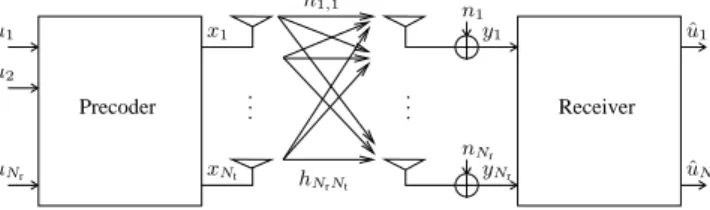
Fig. 1. System with Precoding over Flat MIMO Channel.
algorithm known as Infomax [3] is used when the variation is small.
This work is organized as follows. Sections II describe the signal and system model. Section III presents our method to combine supervised and unsupervised channel estimation and detection. Illustrative computer simulations are presented in Section V and some concluding remarks are made in Section VI.
All derivations are based on the assumption of zero– mean and stationary random variables. Vectors and matrices are denoted by lower case bold and capital bold letters,
respectively. The K×K identity matrix is denoted by IK
and0K is aK-dimensional zero vector. We useE[•],tr(•),
(•)∗, (•)T, (•)H, det(•), and k • k
2, for expectation, trace
of a matrix, complex conjugation, transposition, conjugate transposition, determinant of a matrix, and Euclidean norm,
respectively. Thei-th element of a vectorxisxi.
II. SYSTEMMODEL
We consider a MIMO system with Nt transmit antennas
andNrreceive antennas, as plotted in Figure 1. The precoder
generates the transmit signal x from all data symbols u=
[u1, . . . , uNr] belonging to the different receive antennas 1, . . . , Nr. We denote the equivalent lowpass channel impulse
response between the j–th transmit antenna and the i–
th receive antenna as hi,j(τ, t). Thus, the randomly
time-varying channel is characterized by the Nr ×Nt matrix
H(τ, t)defined as
H(τ, t) =
h1,1(τ, t) h1,2(τ, t) · · · h1,Nt(τ, t)
h2,1(τ, t) h2,2(τ, t) · · · h2,Nt(τ, t)
..
. ... . .. ...
hNr,1(τ, t) hNr,2(τ, t) · · · hNr,Nt(τ, t)
.
Suppose that the transmitted signal from the i–th transmit
u[n] x[n]
η[n]
F H gIˆ
u[n] Q(•) u˜[n]
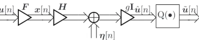
Fig. 2. MIMO System with Linear Transmit Filter (Linear Precoding).
antenna is given by
yj(t) = Nt X
i=1
hj,i(τ, t)∗xi(t) +ηj(t)
where ηj(t) is the additive noise. In matrix notation, this
equation can be rewritten as
y(t) =H(τ, t)∗x(t) +η(t)
where x(t) = [x1(t), . . . , xNt(t)]T ∈ C
Nt,
y(t) = [y1(t), . . . , yNr(t)]T ∈ C
Nr, and η(t) =
[η1(t), . . . , ηNr(t)]T ∈ C
Nr. For flat fading channels,
the channel matrix H(τ, t) is transformed into the matrix
H(t)given by
H(t) =
h1,1(t) h1,2(t) · · · h1,Nt(t)
h2,1(t) h2,2(t) · · · h2,Nt(t)
..
. ... . .. ...
hNr,1(t) hNr,2(t) · · · hNr,Nt(t)
and the received signal is now
yj(t) = Nt X
i=1
hji(t)xi(t) +ηj(t)
which can be expressed in matrix form as
y(t) =H(t)x(t) +η(t). (1)
In general, if we let f[n] =f(nTs+∆) denote samples of
f(t)everyTs seconds with∆being the sampling delay and
Ts the symbol time, then sampling y(t) every Ts seconds
yields the discrete time signaly[n] =y(nTs+∆)given by
y[n] =H[q]x[n] +η(n) (2)
wheren= 0,1,2, . . .corresponds to samples spaced withTs
andqdenotes the slot time. The channel remains unchanged
during a block ofNBsymbols, i.e, over the data frame. Note
that this discrete time model is equivalent to the continuous time model in Equation (1) only if ISI between samples is avoided, i.e. if the Nyquist criterion is satisfied. In that case, we will be able to reconstruct the original continuous signal from the samples by means of interpolation. This channel model is known as time-varying flat block fading channel and this assumption is made in the following.
For brevity, we omit the slot index qin the sequel.
A. Linear Precoding
In this section, we will obtain a form of performing the pre-equalizer (or precoder) step at the transmitter. Since this operation is performed prior to transmission, it is only
possible for a centralized transmitter as in the downlink of a cellular system.
We assume that the receive filter is an identity matrix
(mul-tiplied by a scalarg, withg∈C)allowing for decentralized
receivers). The goal is to find the optimum transmit filterF.
Therefore, the transmit and receive filter are given by the
matrices F ∈CNt×Nr andG =gI∈CNr×Nr, respectively.
In other words, the number of scalar data streams is Nr.
The resulting communications system is shown in Figure 2.
It can be seen from the figure how the data symbols u[n]
are passed through the transmit filterF to form the transmit
signalx[n] =F u[n]∈CNt. Note that the constraint for the
transmit energy must be fulfilled, i.e.
Ehkx[n]k22i= tr F CuFH≤Etx.
The received signal is given by
y[n] =HF u[n] +η[n]∈CNr
where H ∈ CNr×Nt andη[n]∈ CNr is the Additive White
Gaussian Noise (AWGN).
After multiplying by the receive gain g, we get the
estimated symbols
ˆ
u[n] =gHF u[n] +gη[n]∈CNr. (3)
Clearly, the restriction that all the receivers apply the same
scalar weight g is not necessary for decentralized receivers.
ReplacingG by a diagonal matrix suffices (e.g. [4]).
How-ever, usually no closed form can be obtained for the precoder
ifGis diagonal. Fortunately,F can be found in closed form
for G=gI. Thus, we use G=gIin the following.
Although Wiener filtering for precoding has been dealt with by only a few authors [5] in comparison with other criteria for precoding, it is a very powerful transmit opti-mization that minimizes the Mean Square Error (MSE) with a transmit energy constraint [2], [6]–[8], i.e.
{FWF, gWF}= argmin
{F,g}
Ehku[n]−uˆ[n]k22i
s.t.: tr(F CuFH)≤Etx. (4)
In [5], it have been demonstrated that, which leads to a
unique solution if we restrict g to being positive real, the
solution for the Wiener filter is given by
FWF=g−WF1 HHH+ξI
−1
HH
gWF=
v u u ttr
(HHH+ξI)−2HHCuH
Etx
.
(5)
III. ADAPTIVE ALGORITHMS
The model explained in Section II states that the observa-tions are linear and instantaneous mixtures of the transmitted signalsx[n]of Equation (2), i.e.
For the case of the linear precoder described in previous section, this equation can be rewritten as follows
y[n] =HF u[n] +η[n]. (7)
This means that the observations y[n] are instantaneous
mixtures of the data symbolsu[n], where the mixing matrix
is given by HF. For brevity, we will denote this mixing
matrix in the sequel as A, so the observationsy[n] can be
obtained in this way
y[n] =Ad[n] +η[n]. (8)
In accordance with our target, matrix A may represent the
channel matrix [cf. Equation (6)], or the whole coding–
channel matrix, HF [cf. Equation (7)]. In the first case,
d[n] represents the code signal x[n] = F u[n] and, in the
second case, the data one,u[n]. We assume that the mixing
matrix is unknown but full rank nevertheless. Without any loss of generality we can suppose that the source data have a normalized power equal to one since possible differences
in power may be included into the mixing matrixA.
In order to recover the source data, we will use a linear system whose output is a combination of the observations, expressed as
z[n] =WH[n]y[n]. (9)
By combining both Equations (8) and (9), the outputz[n]can
be rewritten as a linear combination of the desired signal
z[n] =Γ[n]d[n] (10)
where Γ[n] = WH[n]A represents the overall
mi-xing/separating system. Sources are optimally recovered
when the matrix W[n] is selected such as every output
extracts a different single source. This occurs when the
matrixG[n]has the form
Γ[n] =D[n]P[n] (11)
where D[n] is a diagonal invertible matrix and P is a
permutation matrix.
A. Supervised Approach
A way to estimate the channel matrix, H, consists on
minimizing the MSE between the outputsy[n]and the code
signals x[n]. Mathematically, using equation (6), the cost
function is written as
JMSE=
NB
X
i=1
E
|zi[n]−di[n]|2
= E
tr (WH[n]y[n]−d[n])(WH[n]y[n]−d[n])H
.
(12)
where the desired signals is obtained from the pilot symbols
u[n]by usingd(n) =F u(n). A way to find the minima of
this cost function consists in using a gradient algorithm that adapt the separating coefficients according with the gradient
of this JMSE, which is given by
∇WJMSE= E
z[n](WH[n]y[n]−d[n])H
. (13)
In general, the expectation included in ∇WJMSE[n] is
un-known so it must be estimated from the available data. In particular, by considering only one sample, we obtain the
Least Mean Squares (LMS) algorithm,
W[n+ 1] =W[n]−µy[n](WH[n]y[n]−d[n])H. (14)
This algorithm is also called delta rule of Widrow-Hopf [9] in the context of Artificial Neural Networks [9]. It is easy to prove that the stationary points of this rule are
W[n] =Rz−1Rzd (15)
where Rz= E[z[n]zH [n]]is the autocorrelation of the
ob-servations and Rzd= E[z[n]dH[n]]is the cross–correlation
between the observations and the desired signals. In practice, the desired signal is considered as known only during a finite number of instants (pilot symbols) and the expectations are estimated by means of using samples averaging.
B. Unsupervised Approach
The inclusion of pilot symbols reduces the system through-put (or equivalently, it reduces the system spectral efficiency) and wastes transmission energy because pilot sequences do not convey information. This limitation can be avoided by using Blind Source Separation (BSS) algorithms which
simultaneously estimate the mixing matrix A and the
real-izations of the source vector u[n] from the corresponding
realizations of the observed vector y[n].
One of the best known BSS algorithms has been ap-proached by Bell and Sejnowski in [3]. Given an activation
functionh(•), the idea proposed by these authors is to obtain
the weighted coefficients of a Neural Network,W[n], in
or-der to maximize the mutual information between the outputs before the activation function, h(z[n]) = h(WH[n]y[n]),
and its inputsy[n], which is given by
JMI(W[n]) = ln(det(WH[n])) +
NB
X
i=1
E[ln(h′
i(zi[n]))] (16)
where hi is the i–th element of the vector h(z[n]) and
′ denotes the first derivative. The maximum of this cost
function can be obtained by means of using a gradient algorithm [3] or a relative gradient algorithm [10], [11]. Both approaches use the gradient of Equation (16) which is obtained as follows
∇WJM I =∇W ln(det(WH[n]))
+∇W
NB
X
i=1
E[ln(h′i(zi[n]))]
!
= adj(WH[n])
det(WH[n])−E[y[n]g
H(z[n])]
=W−H[n]−E[y[n]gH(z[n])] (17)
where adj(•) is the adjunct of a matrix and g(z[n]) =
[−h′′
as before, we obtain the learning rules named gradient
algorithm and relative gradient algorithm and given by
• Gradient Algorithm:
W[n+ 1] =W[n] +µ W−H[n]−y[n]gH(z[n]) =W[n]−µ y[n]gH(z[n])−W−H[n]
(18)
• Relative Gradient Algorithm (Infomax):
W[n+ 1] =W[n] +µW[n]WH[n] · y[n] gH(z[n])−W−H[n] =W[n] +µW[n] z[n]gH(z[n])−I
.
(19)
The expression in Equation (16) admits an interesting in-terpretation by means of the use of the non–linear function
g(z) = z∗(1− |z|2). In this case, Castedo et al. [12] have
shown that the Bell and Sejnowski rules are equivalent to the
Constant Modulus Algorithm (CMA) proposed by Godard in
[13].
IV. HYBRID APPROACH
One of advantage of adaptive unsupervised (or blind) algorithms is their capacity of tracking low variations in the channel. On the contrary, supervised solutions provides a fast channel estimation for low or high variations at the cost of using pilot symbols. In this section, we combine this two parading in order to obtain an performance near to supervised approaches, but using lower number of pilot symbols. Figure 3 shows a simplified block diagram for this hybrid approach.
We will denote by Wu[n] and Ws[n] the matrices of
coefficients for the unsupervised and the supervised module, respectively. We start with an initial estimation of the channel matrix obtained using the Widrow-Hopf solution given by Equation (15). This estimation is used at the transmitter
in order to obtain the optimum coding matrix F and at
the receiver with the goal of initializing the unsupervised algorithm toWu[n] = (F H)−H.
When the “decision module” determines that the channel has not suffered from an important variation, the matrix
Wu[n] is adapted and the data symbols u[n] are recovered
by means of using z[n] = WH
u[n]y[n]. On the contrary, when a considerable variation has occurred, the receiver sends an “alarm” to the transmitter by means of the feedback channel. At this instant, a pilot sequence must be sent by the transmitter. At the receiver, an supervised algorithm estimates the channel from the pilot symbols. In particular, we consider Widrow-Hopf solution of Equation (15) by considering that
u[n] are the coded signals at the linear precoder output.
This solution provides us the channel matrix estimate. This estimation is sent to the transmitter in order to adapt the coding matrix. The receiver also computes the coding matrix
F[n] and the reference matrix HFˆ , and initializes the
unsupervised algorithms such as Wu[n] = ˆHF
−1
A. Decision rule
The question now is how to determine the instant where the channel has suffered a considerable change. An inter-esting consequence of using a linear precoder is that the permutation indeterminacy (see Equation (11)) associated to unsupervised algorithms is avoided because of the
initial-ization to Wu[n] = (F H)−H. This means that the sources
are recovered in the same order as were transmitted. Taking into account, Equation (11) implies that optimum separation
matrix produces a diagonal matrix Γ[n] and, therefore, the
mismatch of Γ[n]with respect to a diagonal matrix allows
us to measure the variations in the channel.
Although the channel matrix is unknown, we can use
the estimation HFˆ computed by the supervised approach
as a reference. This means that at each iteration we can
compute Γ[n] = WH
u[n] ˆHF. Subsequently, the difference
with respect to a diagonal matrix can be obtained using the following “error” index
Error(n) =
NB
X
i=1
NB
X
j=1,j6=i
|γij[n]|2
|γii[n]|2
+|γji[n]|
2
|γii[n]|2
(20)
where γii[n] denotes the i–th element of its diagonal. A
way of decide when the channel has changed consists in
comparing with some threshold t, i.e.
Error(n)> t→Use supervised approach (21)
The next section shows that the inclusion of this simple rule considerably improves the performance of both supervised and unsupervised approaches. Further work deals with de-signing a more “intelligent” decision criterion taking into account information about the environment.
V. EXPERIMENTALRESULTS
In order to show the performance achieved with the proposed combined schemes, we present the results obtained for several computer were performed considering the trans-mission of 8,000 pixels of the image “cameraman” (in tif format with 256 gray levels) using a QPSK and an MIMO system with four transmit and receive antennas. The channel
matrix is updated each 2,000 symbols using the following
model
H= (1−α)H+αHnew (22)
whereHnew is a4×4matrix randomly generated according
to a Gaussian distribution. The SNR has been stated to20dB.
In order to illustrate the form in which our system works using the rule (21), Figure 4 shows the result of evaluating the error measure given in equation (20) given a channel
updating parameterα= 0.1and two values of the threshold:
t = 0.2 and t = 0.5. We can see that the method detects
the changes produced in the channel at instants 2,000, 4,000 and 6,000. The difference in using the two parameters is the delay needed to detect the variation.
F E E D B A C K
C H A N N E L
Yes/No
algorithm
Unsupervised
algorithm
Supervised
Source recovering
x
[
n
]
Recompute
HF
W
u[
n
]
W
s[
n
]
Error(Γ
)
Fig. 3. Block Diagram for the Combined Approach.
0 1000 2000 3000 4000 5000 6000 7000 8000 0
0.1 0.2 0.3 0.4 0.5 0.6 0.7
time instant
Error
α = 0.1
t=0.2 t=0.5
Fig. 4. Evolution of the error index.
.
• A supervised scheme where the Widrow-Hopf solution
(14) is computed using 200 pilot symbols transmitted
each 2,000 symbols.
• The unsupervised algorithm (Infomax) initialized to the
Widrow-Hopf solution. The step size has been fixed to
µ= 0.001.
• The hybrid approach using the decision rule in equation
(21) witht= 0.7. The Widrow-Hopf solution with200
pilot symbols is used to estimate the channel matrix when the error is bigger than this threshold.
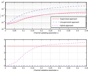
In the first experiment, we have considered that the channel
is updated each NB = 2,000 symbols. This is the best
situation for the supervised approach because implies a perfect synchronization. Figure 5 shows the performance obtained for the three approaches. The results have been obtained by averaging 100 independent realizations. Note that the considerable improvement in the BER obtained for the hybrid approach respect to the unsupervised approach.
It is also apparent that when α < 0.2, the hybrid approach
achieves the same BER than the Wiener-Hopf solution with
less pilot symbols (or, equivalently, number of updating).
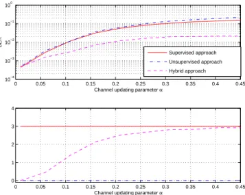
In the second experiment, the number of symbols in which the channel remains constant is a value between 2,000 and 3,000, which is randomly generated for each realizations. Figure 6 plots the BER and the number of updating. Note that the BER of the hybrid approach overcomes to the BER obtained with the other approaches, even the supervised solution, with a reduced number of updating.
Comparing Figure 5 and Figure 6, we observe that the BER of the hybrid system is invariant to the number of symbols in which the channel remains constant and it is obtained a considerable reduction in the number of of times in which the supervised approach is needed. This reduction is due to the fact that the channel remains constant more than 2,000 symbols. Remark also the important loss in quality of the supervised approach due to the outmatching between the channel updating instant and the instant when the pilot symbols are transmitted.
0 0.05 0.1 0.15 0.2 0.25 0.3 0.35 0.4 0.45 10−4
10−3 10−2 10−1 100
Channel updating parameter α
BER
Supervised approach Unsupervised approach Hybrid approach
0 0.05 0.1 0.15 0.2 0.25 0.3 0.35 0.4 0.45 0
1 2 3 4
Channel updating parameter α
Fig. 5. Performance when the channel remains constant during a fixed number of symbolsNB= 2,000.
0 0.05 0.1 0.15 0.2 0.25 0.3 0.35 0.4 0.45 10−4
10−3 10−2 10−1 100
Channel updating parameter α
BER
Supervised approach Unsupervised approach Hybrid approach
0 0.05 0.1 0.15 0.2 0.25 0.3 0.35 0.4 0.45 0
1 2 3 4
Channel updating parameter α
Fig. 6. Performance when the channel remains constant during a randomly generated number of symbols.
.
VI. CONCLUSIONS
In order to reduce the overhead due to the transmission of pilots symbols in FDD-LP systems, we have proposed to combine supervised and unsupervised algorithms. The algorithm selection is done by using a simple decision rule that allows to determine the case when the channel has suffered a considerable variation. This information is sent to the transmitter using the feedback channel. The experiment results show that the hybrid approach is an attractive solution because it provides an adequate BER with a reduced number of pilot symbols. However, thinking in the transmission of an image with good quality, the hybrid approach is adequate when α <0.1.
ACKNOWLEDGMENT
This work was supported by Xunta de Galicia, Ministerio de Educaci´on y Ciencia, Ministerio de Ciencia e Innovaci´on of Spain and FEDER funds of the European Union under grants number 09TIC008105PR, TEC2007-68020-C04-01, CSD2008-00010 and TIN2009-05736-E/TIN.
REFERENCES
[1] R. F. H. Fischer, Precoding and Signal Shaping for Digital
Transmis-sion. John Wiley & Sons, 2002.
[2] M. Joham, Optimization of Linear and Nonlinear Transmit Signal
Processing. PhD dissertation. Munich University of Technology, 2004.
[3] A. Bell and T. Sejnowski, “An information-maximization approach to blind separation and blind deconvolution,” Neural Computation, vol. vol. 7, no. no. 6, pp. pp. 1129–1159, November 1995.
[4] R. Hunger, M. Joham, and W. Utschick, “Extension of linear and nonlinear transmit filters for decentralized receivers,” in European
Wireless 2005, April 2005, pp. 40–46, vol. 1.
[5] M. Joham, K. Kusume, M. H. Gzara, W. Utschick, and J. A. Nossek, “Transmit Wiener Filter for the Downlink of TDD DS-CDMA Sys-tems,” in Proc. ISSSTA, vol. 1, September 2002, pp. 9–13.
[6] R. L. Choi and R. D. Murch, “New Transmit Schemes and Simplified Receiver for MIMO Wireless Communication Systems,” IEEE
Trans-actions on Wireless Communications, vol. 2, no. 6, pp. 1217–1230,
November 2003.
[7] H. R. Karimi, M. Sandell, and J. Salz, “Comparison between Transmit-ter and Receiver Array Processing to Achieve InTransmit-terference Nulling and Diversity,” in Proc. PIMRC, vol. 3, September 1999, pp. 997–1001. [8] J. A. Nossek, M. Joham, and W. Utschick, “Transmit Processing in
MIMO Wireless Systems,” in Proc. of the 6th IEEE Circuits and
Sys-tems Symposium on Emerging Technologies: Frontiers of Mobile and Wireless Communication, May/June 2004, pp. I–18 – I–23, Shanghai,
China.
[9] S. Haykin, Neural Networks A Comprehensive Foundation. Macmillan College Publishing Company, New York, 1994.
[10] S.-I. Amari, “Gradient learning in structured parameter spaces: Adap-tive blind separation of signal sources,” in Proc. WCNN’96. San Diego, 1996, pp. 951–956.
[11] C. Mejuto and L. Castedo, “A neural network approach to blind source separation,” in Proc. Neural Networks for Signal Processing
VII. Florida, USA, September 1997, pp. 486–595.
[12] L. Castedo and O. Macchi, “Maximizing the information transfer for adaptive unsupervised source separation,” in Proc. SPAWC’97. Paris, France, April 1997, pp. 65–68.
[13] D. N. Godard, “Self–recovering equalization carrier tracking in twodi-mensional data communications systems,” IEEE Transactions on