CONTROL THEORY
Volume8, Number3, September2019 pp.489–502
A DYNAMIC PROBLEM INVOLVING A COUPLED
SUSPENSION BRIDGE SYSTEM: NUMERICAL ANALYSIS AND COMPUTATIONAL EXPERIMENTS
Marco Campo
Departamento de Matem´aticas, Universidade da Coru˜na ETS de Ingenieros de Caminos, Canales y Puertos, Campus de Elvi˜na
15071 A Coru˜na, Spain
Jos´e R. Fern´andez∗
Departamento de Matem´atica Aplicada I, Universidade de Vigo ETSI Telecomunicaci´on, Campus As Lagoas Marcosende s/n
36310 Vigo, Spain
Maria Grazia Naso
Dipartimento di Ingegneria Civile, Architettura, Territorio, Ambiente e di Matematica Universit`a degli Studi di Brescia
Via Valotti 9, 25133 Brescia, Italy
(Communicated by Josef Malek )
Abstract. In this paper we study, from the numerical point of view, a dy-namic problem which models a suspension bridge system. This problem is written as a nonlinear system of hyperbolic partial differential equations in terms of the displacements of the bridge and of the cable. By using the respec-tive velocities, its variational formulation leads to a coupled system of parabolic nonlinear variational equations. An existence and uniqueness result, and an exponential energy decay property, are recalled. Then, fully discrete approx-imations are introduced by using the classical finite element method and the implicit Euler scheme. A discrete stability property is shown and a priori error estimates are proved, from which the linear convergence of the algorithm is de-duced under suitable additional regularity conditions. Finally, some numerical results are shown to demonstrate the accuracy of the approximation and the behaviour of the solution.
1. Introduction. During the last decades the study of the so-called suspension bridges has received a large attention because this kind of bridges is a common type of civil engineering structure. It is well-known that these bridges may display certain oscillations under external aerodynamic forces like, for instance, it occurred in the famous Tacoma’s bridge (see [2, 5]), in which a strong wind caused the collapse of a narrow and very flexible suspension bridge.
2000Mathematics Subject Classification. Primary: 74B20, 65M60, 65M15; Secondary: 74K10, 74H15.
Key words and phrases. Coupled bridge system, finite elements, a priori error estimates, nu-merical simulations.
This work has been supported by Ministerio de Econom´ıa y Competitividad under the project MTM2015-66640-P (with the participation of FEDER).
∗Corresponding author: Jos´e R. Fern´andez.
Since the pioneering works by Lazer and McKenna (see, e.g., [14] or [18]), where mathematical models based on nonlinear partial differential equations were intro-duced to describe oscillations in suspension bridges including connection cables, a large number of papers have been published (see, for instance, [1,3,10,11,12,13, 16, 19, 20, 21, 22, 23, 24, 25] and the numerous references cited therein). Most of the above works deal with mathematical aspects as the application of analytical methods to scrutinize stationary solutions, periodic oscillations, longtime global dy-namics, existence and uniqueness of solutions and so on. Moreover, we want to point out that in the literature other types of suspension bridges were studied, where the associated dynamic system was written in the vertical and torsional displacements of a cross-section of the bridge (see, e.g., [4, 15]). However, to our knowledge the numerical analyses of the proposed models have not been performed yet.
In this paper, we revisit the problem considered in [7], where a model taking into account the coupling between the road bed and the suspension main cable was studied from the mathematical point of view, proving the existence and unique-ness of weak solutions by using the Faedo-Galerkin approximation procedure and Gronwall’s lemma, and the exponential decay of the system energy. Moreover, the existence of a regular global attractor was also shown by using the semigroup the-ory and defining an adequate Lyapunov functional. Here, we aim to provide the numerical analysis of this dynamic problem, introducing fully discrete approxima-tions, proving a discrete stability result and a priori error estimates, and performing numerical simulations which demonstrate the accuracy of the algorithm and the be-haviour of the solution.
The paper is outlined as follows. The mathematical model is described in Section 2 following [7], deriving its variational formulation. An existence and uniqueness result, and an energy decay property, proved in [7] are also stated. Then, in Sec-tion 3 a numerical scheme is introduced, based on the finite element method to approximate the spatial domain and the forward Euler scheme to discretize the time derivatives. A discrete stability property is proved and a priori error estimates are deduced for the approximative solutions from which, under suitable regularity assumptions, the linear convergence of the algorithm is obtained. Finally, some numerical simulations are presented in Section4.
2. The model and its variational formulation. In this section, we present briefly the model, the required assumptions and the variational formulation of the mechanical problem, and we state an existence and uniqueness result. We refer the reader to [7] for details.
Let [0, `], ` >0, be the one-dimensional beam (bridge) or rod (cable) of length
`and denote by [0, T],T >0, the time interval of interest. Moreover, letx∈[0, `] and t∈ [0, T] be the spatial and time variables, respectively. In order to simplify the writing, we do not indicate the dependence of the functions onxandt, and a subscript under a variable represents its derivative with respect to the prescribed variable.
Problem P.Find the bending displacement u: [0, `]×[0, T]→Rand the vertical
displacementw: [0, `]×[0, T]→Rsuch that
utt+uxxxx+ut+ (p− kuxk2L2(0,`))uxx+k2∗(u−w)+=f (1)
in (0, `)×(0, T), (2)
wtt−wxx+wt−k∗2(u−w)
+=g in (0, `)
×(0, T), (3)
u(0, t) =u(`, t) =ux(0, t) =ux(`, t) = 0 for a.e. t∈(0, T), (4)
w(0, t) =w(`, t) = 0 for a.e. t∈(0, T), (5)
u(x,0) =u0(x), ut(x,0) =v0(x) for a.e. x∈(0, `), (6)
w(x,0) =w0(x), wt(x,0) =e0(x) for a.e. x∈(0, `). (7)
Here, the notation (F)+ stands for the positive part of a functionF, i.e. (F)+= max{0, F}. Moreover, the term−k∗2(u−w)+ models a restoring force due to the cables, f is the given vertical dead load distribution on the deck, the constantp
represents the axial force acting at the ends of the road bed in the reference configu-ration (being negative when the bridge is stretched and positive when compressed), andg denotes an external source applied in the cable. Finally, following [7] we as-sumed that all the constants in the model were equal to 1 for the sake of simplicity in the writing. However, in order to simplify the calculations in this work we note that we have modified slightly the boundary conditions employed in [7], where the ends of the vibrating beam were considered pinned, assuming instead that they are rigidly fixed now. The analysis performed there could be adapted with some minor changes.
In order to obtain the variational formulation of Problem P, let Y = L2(0, `) and denote by (·,·) the scalar product in this space, with corresponding normk · k. Moreover, let us define the variational spacesV andE as follows,
V ={v∈H2(0, `) ;v(0) =v(`) = 0 andv
x(0) =vx(`) = 0},
E={e∈H1(0, `) ;e(0) =e(`) = 0},
with scalar product (·,·)V (resp. (·,·)E) and normk · kV (resp. k · kE) defined inV
(resp. E).
By using the integration by parts and the Dirichlet boundary conditions atx= 0, `, we write the variational formulation of Problem P in terms of the bending velocityv=ut and the vertical velocitye=wt.
Problem VP. Find the bending velocity v : [0, T] → V and the vertical velocity e: [0, T]→E such that v(0) =v0,e(0) =e0 and, for a.e. t∈(0, T),
(vt(t), ξ) + (uxx(t), ξxx) + (v(t), ξ) +kux(t)k2(ux(t), ξx) +p(uxx(t), ξ)
+k∗2((u(t)−w(t))+, ξ) = (f(t), ξ) ∀ξ∈V, (8) (et(t), ψ) + (wx(t), ψx) + (e(t), ψ)−k2∗((u(t)−w(t))
+, ψ)
= (g(t), ψ) ∀ψ∈E, (9)
where the bending displacement and the vertical displacement are then recovered from the relations:
u(t) =
Z t
0
v(s)ds+u0, w(t) =
Z t
0
The following theorem has been proved in [7], providing the existence of a unique solution to Problem VP as well as an energy decay property.
Theorem 2.1. Let f, g ∈ C([0, T];Y) and assume that the initial data have the regularity
u0∈H2(0, `), v0∈Y, w0∈E, e0∈Y.
Then, there exists a unique solution to Problem VP with the following regularity:
u∈C([0, T];H2(0, `)), v∈C([0, T];Y),
w∈C([0, T];H1(0, `)), e∈C([0, T];Y).
Moreover, this solution is continuously dependent on the given data.
In addition, if we assume thatf =g= 0 (i.e. there are not volume forces) and that the axial force p is small enough, denoting by E(t) the energy of the system given by
E(t) =ku(t)k2V +kv(t)k
2
+kw(t)k2E+ke(t)k
2
,
then it decays exponentially; i.e. there exist two positive constants Q and ω such that
E(t)≤Q e−ω t, t≥0.
3. Numerical analysis: Fully discrete approximations and a priori error estimates. In this section we consider a fully discrete approximation of Problem VP. This is done in two steps. First, we assume that the interval [0, `] is divided into
M subintervalsa0= 0< a1< . . . < aM =` of lengthh=ai+1−ai=`/M and so,
to approximate the variational spacesV andE, we construct the finite dimensional spacesVh⊂V andEh⊂E given by
Vh={ξh∈C1([0, `]) ; ξh|
[ai,ai+1 ]
∈P3([ai, ai+1]) i= 0, . . . , M−1,
ξh(0) =ξh(`) = 0 andξxh(0) =ξhx(`) = 0}, (11)
Eh={ψh∈C([0, `]) ; ψ|h
[ai,ai+1 ] ∈P1([ai, ai+1]) i= 0, . . . , M−1,
ψh(0) =ψh(`) = 0}, (12)
wherePr([ai, ai+1]) represents the space of polynomials of degree less or equal torin the subinterval [ai, ai+1]; i.e. Vh is composed of C1 and piecewise cubic functions and Eh is composed of continuous and piecewise affine functions. Here, h > 0
denotes the spatial discretization parameter. Moreover, we assume that the discrete initial conditions, denoted byuh
0,vh0,wh0 andeh0, are given by
uh0 =P1hu0, vh0 =P
h
1v0, wh0 =P
h
2w0, eh0 =P
h
2e0. (13) Ph
1 and P2h being the classical finite element interpolation operators over Vh and
Eh, respectively (see [9]).
Secondly, we consider a partition of the time interval [0, T], denoted by 0 =
t0 < t1 < · · · < tN = T. In this case, we use a uniform partition with step
size k =T /N and nodes tn =n k for n= 0,1, . . . , N. For a continuous function
z(t), we use the notation zn = z(tn) and, for a sequence {wn}Nn=0, we denote by
δwn= (wn−wn−1)/k its divided differences.
Problem VPhk. Find the discrete bending velocityvhk ={vnhk}N n=0⊂V
h and the
discrete vertical velocity ehk ={ehkn }N n=0 ⊂E
h such that vhk
0 =v
h
0, e
hk
0 =e
h
0 and,
forn= 1, . . . , N,
(δvhkn , ξh) + ((uhkn )xx, ξxxh ) + (v hk n , ξ
h) +k(uhk
n )xk2((uhkn )x, ξhx) +p((u hk n )xx, ξh)
+k2∗((uhkn −wnhk)+, ξh) = (fn, ξh) ∀ξh∈Vh, (14)
(δehkn , ψh) + ((whkn )x, ψxh) + (e hk n , ψ
h)−k2
∗((uhkn −w hk n )
+, ψh)
= (gn, ψh) ∀ψh∈Eh, (15)
where the discrete bending displacement and the discrete vertical displacement are then recovered from the relations:
uhkn =k
n
X
j=1
vjhk+uh0, wnhk=k
n
X
j=1
ehkj +w0h. (16)
The existence of a unique solution to Problem VPhk can be obtained procee-ding as in the continuous case, applying a standard Faedo-Galerkin approximation procedure (see, for instance, [6, 17]).
The aim of this section is to obtain some a priori error estimates on the numerical errorsun−uhkn , vn−vnhk,wn−wnhk anden−ehkn .
Now, we have the following discrete stability property.
Lemma 3.1. Let the assumptions of Theorem2.1 hold. Then, the numerical se-quences {uhk, vhk, whk, ehk}, generated by Problem V Phk, satisfy the stability
esti-mate:
kvnhkk2+kuhk n k
2
V +k(u hk
n )xk4+kehkn k
2+kwhk n k
2
E≤C,
whereCis a positive constant which is independent of the discretization parameters handk.
Proof. In order to simplify the writing of this proof, we remove the superscriptsh
andkin all the variables and we assume thatf =g= 0. Taking as a test functionξh=v
n in equation (14) we have
(δvn, vn) + ((un)xx,(vn)xx) + (vn, vn) +k(un)xk2((un)x,(vn)x) +p((un)xx, vn)
+k2
∗((un−wn)+, vn) = 0.
Now, keeping in mind that
(δvn, vn)≥
1 2k
kvnk2− kvn−1k2 ,
k2∗((un−wn)+, vn)≤k2∗(kunk2+kwnk2+kvnk2),
k(un)xk2((un)x,(vn)x) =
1
kk(un)xk
2((u
n)x,(un−un−1)x)
≥ 1 4k
k(un)xk4− k(un−1)xk4 ,
p((un)xx, vn)≤
|p|
2 (k(un)xxk 2+
kvnk2),
((un)xx,(vn)xx)≥
1 2k
k(un)xxk2− k(un−1)xxk2 ,
where we used Cauchy-Schwarz and Young inequalities, it follows that 1
2k
kvnk2− kvn−1k2 + 1 4k
k(un)xk4− k(un−1)xk4
+ 1 2k
k(un)xxk2− k(un−1)xxk2
≤C(kunk2+kwnk2+kvnk2+k(un)xxk2).
Now, takingψh=en as a test function in equation (15) we find that
(δen, en) + ((wn)x,(en)x) + (en, en)−k2∗((un−wn)+, en) = 0,
and so, taking into account that
(δen, en)≥
1 2k
kenk2− ken−1k2 ,
((wn)x,(en)x)≥
1 2k
k(wn)xk2− k(wn−1)xk2 ,
k2
∗((un−wn)+, en)≤k∗2(kunk2+kwnk2+kenk2),
we have
1 2k
kenk2− ken−1k2 +
1 2k
k(wn)xk2− k(wn−1)xk2
≤C(kunk2+kwnk2+kenk2).
(18)
Combining now (17) and (18) we can conclude that
1 2k
kvnk2− kvn−1k2 + 1 4k
k(un)xk4− k(un−1)xk4
+ 1 2k
k(un)xxk2− k(un−1)xxk2 +
1 2k
kenk2− ken−1k2 + 1
2k
k(wn)xk2− k(wn−1)xk2
≤C(kunk2+kwnk2+kvnk2+kenk2+k(un)xxk2).
Thus, by induction and using Poincare’s inequality we find that
kvnk2+k(un)xk4+kunk2V +kenk2+kwnk2E
≤Ck
n
X
j=1
(kujk2V +kvjk2+kwjk2E+kejk2)
+C(kv0k2+ku0k2
V +ke0k
2+kw0k2
E),
and, applying a discrete version of Gronwall’s inequality (see, for instance, [8]) we find the desired stability estimates.
Remark 1. We note that we could modify Problem VPhk by using a semi-implicit scheme in the following form:
Find the discrete bending velocityvhk ={vhk
n }Nn=0⊂Vh and the discrete vertical
velocityehk ={ehk
n }Nn=0⊂Eh such that vhk0 =v0h,ehk0 =eh0 and, for n= 1, . . . , N, (δvnhk, ξh) + ((uhkn )xx, ξxxh ) + (v
hk n , ξ
h) +k(uhk
n−1)xk2((unhk)x, ξxh) +p((u hk n )xx, ξh)
+k∗2((uhkn−1−whkn−1)+, ξh) = (fn, ξh) ∀ξh∈Vh,
(δehkn , ψh) + ((wnhk)x, ψhx) + (ehkn , ψh)−k2∗((uhkn−1−wnhk−1)+, ψh) = (gn, ψh) ∀ψh∈Eh,
where the discrete bending displacement and the discrete vertical displacement are again recovered from relations (16).
This new problem is now uncoupled and linear and so, the numerical resolution is easier. However, Lemma3.1should be modified and the resulting estimates will vary accordingly.
Theorem 3.2. Let the assumptions of Theorem 2.1 still hold and denote by(v, e)
and (vhk, ehk)the solutions to problems VP and V Phk, respectively. Assume that the following additional regularity is satisfied:
v∈C1([0, T];Y)∩C([0, T];V), e∈C1([0, T];Y)∩C([0, T];E). Then we have the following a priori error estimates, for allξh={ξh
j}Nj=0⊂Vhand
ψh={ψjh}N j=0⊂E
h,
max 0≤n≤N
n
kvn−vnhkk2+ken−ehkn k2+kun−uhkn k2V +kwn−whkn k2E
o ≤Ck N X j=1
k(vt)j−δvjk2+kvj−ξjhk
2
V +k(ut)j−δujkV2 +k(et)j−δejk2
+kej−ψjhk
2
E+k(wt)j−δwjk2E
+Ckv0−v0hk 2+
ke0−eh0k 2
+ku0−uh0k 2
V +kw0−wh0k 2
E
+C
k
N−1
X
j=1
kvj−ξjh−(vj+1−ξjh+1)k 2
+C
k
N−1
X
j=1
kej−ψjh−(ej+1−ψhj+1)k
2+C max
0≤n≤Nkvn−ξ h nk
2
+C max
0≤n≤Nken−ψ h nk
2. (19)
Proof. Taking as a test functionξ=ξh ∈Vh ⊂V in equation (8) at time t =tn
and subtracting it to equation (14) we have
((vt)n−δvhkn , ξh) + ((un−uhkn )xx,(ξh)xx) + (vn−vnhk, ξh)
+ k(un)xk2(un)x− k(unhk)xk2(unhk)x,(ξh)x
+p((un−uhkn )xx, ξh)
+k2
∗((un−wn)+−(uhkn −wnhk)+, ξh) = 0,
and therefore,
((vt)n−δvhkn , vn−vnhk) + ((un−uhkn )xx,(vn−vhkn )xx) + (vn−vhkn , vn−vnhk)
+ k(un)xk2(un)x− k(uhkn )xk2(uhkn )x,(vn−vnhk)x
+p((un−uhkn )xx, vn−vnhk)
+k∗2((un−wn)+−(uhkn −w hk n )
+, v
n−vhkn )
= ((vt)n−δvnhk, vn−ξh) + ((un−uhkn )xx,(vn−ξh)xx) + (vn−vnhk, vn−ξh)
+ k(un)xk2(un)x− k(uhkn )xk2(uhkn )x,(vn−ξh)x+p((un−uhkn )xx, vn−ξh)
+k2
∗((un−wn)+−(uhkn −wnhk)+, vn−ξh) ∀ξh∈Vh.
Taking into account that
(δvn−δvnhk, vn−vhkn )≥
1 2k
kvn−vnhkk
2− kv
n−1−vnhk−1k 2 , ((un−uhkn )xx,(vn−vnhk)xx) = ((un−uhkn )xx,((ut)n−δun)xx)
+((un−uhkn )xx,(δun−δuhkn )xx)
≥((un−uhkn )xx,((ut)n−δun)xx)
+21k
k(un−uhkn )xxk2− k(un−1−uhkn−1)xxk2 ,
k(un)xk2(un)xx− k(uhkn )xk2(uhkn )xx, w
= (k(un)xk2− k(unhk)xk2)(un)xx, w
+ k(uhk
n )xk2(un−uhkn )xx, w
,
|(k(uhk
n )xk2(un−uhkn )xx, w)| ≤C(k(un−uhkn )xxk2+kwk2),
where we used Lemma3.1and the notationδun= (un−un−1)/k, and the following
estimates
| (k(un)xk2− k(unhk)xk2)(un)xx, w
| ≤
k(un)xk2− k(uhkn )xk2
≤Ckwk2+C k(u
n)xk2− k(uhkn )xk2
2 ,
k(un)xk2− k(uhkn )xk2=
Z `
0
(un)2x−(u hk n )
2
xdx
=
Z `
0
(un+uhkn )x(un−uhkn )xdx
≤ k(un+uhkn )xkk(un−unhk)xk ≤Ck(un−uhkn )xk,
where the regularityu∈C([0, T];V) and Cauchy’s inequality
ab≤a2+ 1 4b
2, a, b, ∈
R, >0,
have been used, we find that 1
2k
kvn−vnhkk
2− kv
n−1−vnhk−1k 2
+ 1 2k
k(un−uhkn )xxk2− k(un−1−uhkn−1)xxk2
≤Ck(vt)n−δvnk2+kvn−ξhk2+k(vn−ξh)xxk2+k((ut)n−δun)xxk2
+kvn−vnhkk
2+ku
n−uhkn k
2+kw
n−whkn k
2+k(u
n−uhkn )xk2
+k(un−uhkn )xxk2+ (δvn−δvhkn , vn−ξh)
∀ξh∈Vh. (20)
Now, taking as a test function ψ =ψh ∈ Eh ⊂E in equation (9) at timet =tn
and subtracting it from equation (15) we have
((et)n−δehkn , ψ
h) + ((w
n−wnhk)x, ψhx)−k
2
∗((un−wn)+−(uhkn −w hk n )
+, ψh)
+(en−ehkn , ψh) = 0 ∀ψh∈Eh,
and so, we obtain, for allψh∈Eh,
((et)n−δehkn , en−ehkn ) + ((wn−whkn )x,(en−ehkn )x) + (en−ehkn , en−ehkn )
−k2
∗((un−wn)+−(unhk−whkn )+, en−ehkn )
= ((et)n−δehkn , en−ψh) + ((wn−wnhk)x,(en−ψh)x) + (en−ehkn , en−ψh)
−k2
∗((un−wn)+−(unhk−whkn )+, en−ψh).
Keeping in mind that
(δen−δehkn , en−ehkn )≥
1 2k
ken−ehkn k
2− ke
n−1−ehkn−1k 2 , ((wn−whkn )x,(en−ehkn )x) = ((wn−whkn )x,((wt)n−δwn)x)
+((wn−wnhk)x,(δwn−δwhkn )x)
≥((wn−whkn )x,((wt)n−δwn)x) +
1 2k
k(wn−wnhk)xk2− k(wn−1−wnhk−1)xk2 ,
where δwn = (wn−wn−1)/k, using several times the above Cauchy’s inequality it
follows that 1 2k
ken−ehkn k
2− ke
n−1−ehkn−1k 2
+ 1 2k
k(wn−wnhk)xk2− k(wn−1−wnhk−1)xk2
≤Ck(et)n−δenk2+ken−ehkn k2+kwn−whkn k2+kun−uhkn k2
+ken−ψhk2+k(en−ψh)xk2+k((wt)n−δwn)xk2
+(δen−δehkn , en−ψh)
Combining estimates (20) and (21) we have, for allξh∈Vh andψh∈Eh,
1 2k
kvn−vhkn k
2− kv
n−1−vhkn−1k 2 + 1
2k
ken−ehkn k
2− ke
n−1−ehkn−1k 2 + 1
2k
k(un−uhkn )xxk2− k(un−1−uhkn−1)xxk2
+ 1 2k
k(wn−whkn )xk2− k(wn−1−whkn−1)xk2
≤Ck(vt)n−δvnk2+kvn−ξhk2+k(vn−ξh)xxk2+k((ut)n−δun)xxk2
+kvn−vnhkk2+kun−uhkn k2+kwn−whkn k2+k(un−uhkn )xk2
+k(un−uhkn )xxk2+ (δvn−δvnhk, vn−ξh) +k(et)n−δenk2
+ken−ehkn k2+ken−ψhk2+k(en−ψh)xk2+k((wt)n−δwn)xk2
+(δen−δehkn , en−ψh)
.
Thus, by induction we obtain, for allξh={ξjhkN j=0⊂V
handψh={ψh jk
N j=0⊂E
h,
kvn−vnhkk
2+ke
n−ehkn k
2+k(u
n−uhkn )xxk2+k(wn−whkn )xk2
≤Ck
n
X
j=1
k(vt)j−δvjk2+kvj−ξjhk
2+k(v
j−ξhj)xxk2+k((ut)j−δuj)xxk2
+kvj−vhkj k2+kuj−uhkj k2+kwj−wjhkk2+k(uj−uhkj )xk2
+k(uj−uhkj )xxk2+ (δvj−δvjhk, vj−ξjh) +k(et)j−δejk2
+kej−ehkj k2+kej−ψhjk2+k(ej−ψhj)xk2+k((wt)j−δwj)xk2
+(δej−δehkj , ej−ψjh)
+Ckv0−v0hk2+ke0−eh0k2 +k(u0−uh0)xxk2+k(w0−w0h)xk2
.
Finally, taking into account that
k
n
X
j=1
(δvj−δvjhk, vj−ξjh)
=
n
X
j=1
(vj−vhkj −(vj−1−vhkj−1), vj−ξjh)
= (vn−vhkn , vn−ξhn) + (v h
0 −v0, v1−ξ1h) +
n−1
X
j=1
(vj−vhkj , vj−ξjh−(vj+1−ξhj+1)),
k
n
X
j=1
(δej−δehkj , ej−ψhj)
=
n
X
j=1
(ej−ehkj −(ej−1−ehkj−1), ej−ψhj)
= (en−ehkn , en−ψnh) + (e h
0 −e0, e1−ψ1h) +
n−1
X
j=1
(ej−ehkj , ej−ψjh−(ej+1−ψjh+1)),
applying a discrete version of Gronwall’s inequality (see again [8]) and Poincare’s inequality, we conclude estimates (19).
u∈H3(0, T;Y)∩C1([0, T];H3(0, `))∩H2(0, T;V),
w∈H3(0, T;Y)∩C1([0, T];H2(0, `))∩H2(0, T;E). (22) We note that with this regularity we immediately find that (see [9]):
kv0−vh0k 2+ke
0−eh0k 2+ku
0−uh0k 2
V +kw0−w0hk 2
E≤Ch
2. Therefore, we have the following.
Corollary 1. Let the assumptions of Theorem 3.2 and the additional regularity (22) hold. Then, the linear convergence of the algorithm is deduced; i.e. there exists a positive constant C, independent of the discretization parameters h andk, such that
max 0≤n≤N
n
kvn−vhkn k+ken−ehkn k+kun−uhkn kV +kwn−whkn kE
o
≤C(h+k).
The proof of the above result is done in several steps. First, we have the following property of approximation by finite elements (see, e.g., [9]):
k N X j=1 inf ξh j∈Vh
kvj−ξjhk
2
V + inf ψh
j∈Eh
kej−ψhjk
2
E
+ max 0≤n≤Nξhinf
n∈Vh
kvn−ξnhk
2
+ max 0≤n≤Nψhinf
n∈Eh
ken−ψnhk2≤Ch2
kuk2
C1([0,T];H3(0,`))+kwk2C1([0,T];H2(0,`))
.
Moreover, using again regularity conditions (22), we have
k
N
X
j=1
h
k(ut)j−δujkV2 +k(wt)j−δwjkE2 +k(vt)j−δvjk2+k(et)j−δejk2
i
≤Ck2 kuk2
H2(0,T;V)+kuk2H3(0,T;Y)+kwk2H2(0,T;E)+kwk2H3(0,T;Y)
.
Finally, the remaining terms in estimates (19) can be bounded as follows (see [8] for details),
1
k
N−1
X
j=1
kvj−ξhj −(vj+1−ξhj+1)k 2+1
k
N−1
X
j=1
kej−ψhj −(ej+1−ψjh+1)k 2
≤Ch2kuk2
H2(0,T;V)+kwk2H2(0,T;E)
.
Combining all these estimates, the linear convergence is deduced.
4. Numerical results. In order to verify the behaviour of the numerical method described in the previous section, some numerical experiments have been performed. Moreover, for the sake of generality in the simulations, we have included coefficients in the definition of the mechanical problem P.
4.1. Numerical scheme. Given the solution uhkn−1, vhkn−1, whkn−1 and ehkn−1 at time
tn−1,the discrete bending velocity is obtained from the discrete nonlinear variational equation
ρ1(vnhk, ξh) +k2a1((vhkn )xx, ξxxh ) +k c1(v hk n , ξ
h)
+k2r1k(uhkn )xk2((uhkn−1+k v
hk n )x, ξxh)
−k2p((vhkn )x,(ξh)x) +k k∗2((uhkn −whkn )+, ξh) =ρ1(vnhk−1, ξh) +k(fn, ξh)
−k a1((uhkn−1)xx, ξxxh ) +k p((u hk
n−1)x,(ξh)x).
ρ2(ehkn , ψ h
) +k2a2((ehkn )x, ψxh) +c2k(ehkn , ψ h
)−k k∗2((uhkn −w hk n )
+
, ψh)
=ρ2(ehkn−1, ψh) +k(gn, ψh)−k a2((whkn−1)x, ψxh),
where the discrete bending displacement and the discrete vertical displacement are then recovered from the relations
uhkn =k
n
X
j=1
vhkj +uh0, wnhk=k
n
X
j=1
ehkj +wh0.
We note that both numerical problems consist of nonlinear symmetric systems, and so a fixed point method was applied for their solution.
4.2. A first example: Numerical convergence. Our aim with this first example is to verify the numerical convergence of the numerical scheme. In this sense, the following problem is considered.
Problem P1. Find a bending velocity field v : [0,1]×[0,1] 7→ R and a vertical
velocitye: [0,1]×[0,1]7→Rsuch that
ρ1utt+a1uxxxx+c1ut+ (p−r1kuxk2L2(0,`))uxx+k2∗(u−w)
+=f
in (0,1)×(0,1),
ρ2wtt−a2wxx+c2wt−k∗2(u−w)+=g in (0,1)×(0,1), u(0, t) =u(1, t) =ux(0, t) =ux(1, t) = 0 for a.e. t∈(0,1),
w(0, t) =w(1, t) = 0 for a.e. t∈(0,1),
u(x,0) =u0(x), ut(x,0) =v0(x) for a.e. x∈(0,1),
w(x,0) =w0(x), wt(x,0) =e0(x) for a.e. x∈(0,1). where
f(x, t) =et −16x4+ 32x3−12x2−4x−384
+ 16e2t512
105 12x
2−12x+ 2 ,
g(x, t) =et 16x4−32x3+ 28x2−12x−8 ,
which corresponds with Problem P with the following data:
l= 1, T = 1s, ρ1= 1 =ρ2, a1= 1 =a2, c1= 1 =c2, r1= 1, p= 0,
k2∗= 1, u0(x) =−16x2(1−x)2=v0(x) for all x∈(0,1), w0(x) =−4x(1−x) =e0(x) for all x∈(0,1).
The exact solution to Problem P1 is the following one.
u(x, t) =−16x2(1−x)2et, w(x, t) =−4x(1−x)et, for (x, t)∈[0,1]×[0,1].
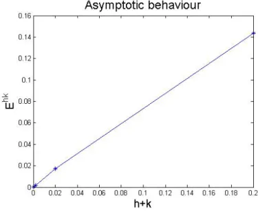
The numerical errors given by
Ehk = max 0≤n≤N
n
kvn−vnhkk+ken−ehkn k+kun−uhkn kV +kwn−wnhkkE
o ,
and obtained for different discretization parametersndandk, are depicted in Table 1 (being nd the number of finite elements of the discretization andh= 1
nd↓k→ 10−1 10−2 10−3 10−4 10 0.1435116 0.0868544 0.0923330 0.0940042 102 0.1639226 0.0174114 0.0070235 0.0069553 103 0.1641941 0.0161108 0.0017435 0.0007232 104 0.1646557 0.0163375 0.0015935 0.0001722
Table 1. Example 1: Numerical errors for some discretization parameters.
Figure 1. Example 1: Asymptotic behaviour of the numerical scheme
4.3. A second example: The effect of the axial force. As a second test several simulations with different values of the axial force p have been performed. With this example we try to show the effect of the axial force on a vibrating situation. Taking a similar forced deformed initial configuration as in the previous example, both forces, over the bridge and the cable, are released at instantt = 0, and the evolution of the bending displacements is studied.
The following data have been used in this example.
l= 1, T = 1s, ρ1= 1 =ρ2, a1= 1 =a2, c1= 10 =c2,
r1= 1, k∗2= 1, f =g= 0,
u0(x) =−16x2(1−x)2=w0(x), v0(x) = 0 =e0(x), for all x∈(0,1).
Using the discretization parameters k =h = 10−3, in Fig. 2 the evolution in time of the vertical displacement of the bridge center is shown for several values of the axial force p. As can be observed, the increment in the compression forces makes the oscillating response to be softer when the bridge is released.
Figure 2. Example 2: Oscillations of the bridge for different
val-ues of p.
The following data have been used in the simulations:
l= 1, T = 1s, ρ1= 1 =ρ2, a1= 1 =a2, c1= 10 =c2, r1= 1,
p= 10, f(x, t) = 10t, g(x, t) = 0, for (x, t)∈[0,1]×[0,1]
u0(x) = 0, v0(x) = 0, w0(x) = 0, e0(x) = 0 for all x∈(0,1).
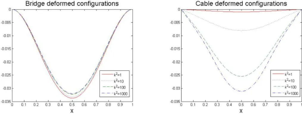
Taking the discretization parametersk=h= 10−3, running several simulations for different values ofk2
∗ the effect of the coupling term is easily noticed: when this
value raises, the cable restricts the deformation of the bridge and so the displacement decreases, while at the same time the cable deformation increases, as can be seen in Fig. 3.
Figure 3. Example 3: Bridge and cable deformed configurations
at final time for different values ofk2
∗.
REFERENCES
[2] O. H. Amann, T. Von Karman and G. B. Wooddruff, The failure of the Tacoma narrows bridge, Federal Works Agency, Washington D.C., 1941.
[3] A. Arena and W. Lacarbonara,Nonlinear parametric modeling of suspension bridges under aerolastic forces: torsional divergence and flutter,Nonlinear Dyn.,70(2012), 2487–2510.
[4] G. Arioli and F. Gazzola,A new mathematical explanation of what triggered the catastrophic torsional mode of the Tacoma Narrows Bridge,Appl. Math. Model.,39(2015), 901–912.
[5] G. Arioli and F. Gazzola,Torsional instability in suspension bridges: The Tacoma Narrows Bridge case,Commun. Nonlinear Sci. Numer. Simul.,42(2017), 342–357.
[6] J. M. Ball,Initial-boundary value problems for an extensible beam,J. Math. Anal. Appl.,42 (1973), 61–90.
[7] I. Bonicchio, C. Giorgi and E. Vuk, Long-term dynamics of the coupled suspension bridge system,Math. Models Methods Appl. Sci.,22(2012), 1250021, 22pp.
[8] M. Campo, J. R. Fern´andez, K. L. Kuttler, M. Shillor and J. M. Via˜no,Numerical analysis and simulations of a dynamic frictionless contact problem with damage,Comput. Methods Appl. Mech. Engrg.,196(2006), 476–488.
[9] P. G. Ciarlet, Basic error estimates for elliptic problems. inHandbook of Numerical Analysis (eds. P.G. Ciarlet and J.L. Lions), Elsevier,II(1993), 17–351.
[10] F. Dell’Oro, C. Giorgi and V. Pata,Asymptotic behaviour of coupled linear systems modeling suspension bridges,Z. Angew. Math. Phys.,66(2015), 1095–1108.
[11] Z. Ding,Traveling waves in a suspension bridge system,SIAM J. Math. Anal.,35(2003), 160–171.
[12] P. Dr´abek, H. Holubov´a, A. Matas and P. Necesal,Nonlinear models of suspension bridges: discussion of the results,Appl. Math.,48(2003), 497–514.
[13] A. Ferrero and F. Gazzola, A partially hinged rectangular plate as a model for suspension bridges,Discrete Contin. Dyn. Syst. Ser. A,35(2015), 5879–5908.
[14] J. Glover, A. C. Lazer and P. J. McKenna, Existence and stability of large scale nonlinear oscillations in suspension bridges,Z. Angew. Math. Phys.,40(1989), 172–200.
[15] D. Green and W. G. Unruh,The failure of the Tacoma bridge: A physical model,Amer. J. Phys.,74(2006), 706–716.
[16] G. Holubov´a-Tajcov´a,Mathematical modeling of suspension bridges,Math. Comput. Simul., 50(1999), 183–197.
[17] G. Holubov´a and A. Matas, Initial-boundary value problem for the nonlinear string-beam system,J. Math. Anal. Appl.,288(2003), 784–802.
[18] A. C. Lazer and P. J. McKenna,Large-amplitude periodic oscillations in suspension bridges: Some new connections with nonlinear analysis,SIAM Rev.,32(1990), 537–578.
[19] H. Leiva, Exact controllability of the suspension bridge model proposed by Lazer and McKenna,J. Math. Anal. Appl.,309(2005), 404–419.
[20] J. Mal´ık,Nonlinear models of suspension bridges,J. Math. Anal. Appl.,321(2006), 828–850. [21] J. Mal´ık, Sudden lateral asymmetry and torsional oscillations in the original Tacoma
suspen-sion bridge,J. Sound Vib.,332(2013), 3772–3789.
[22] J. Mal´ık,Spectral analysis connected with suspension bridge systems,IMA J. Appl. Math., 81(2016), 42–75.
[23] C. Marchionna and S. Panizzi, An instability result in the theory of suspension bridges, Nonlinear Anal.,140(2016), 12–28.
[24] P. J. McKenna, Oscillations in suspension bridges, vertical and torsional,Discrete Contin. Dyn. Syst. Ser. S,7(2014), 785–791.
[25] C. Zhong, Q. Ma and C. Sun, Existence of strong solutions and global attractors for the suspension bridge equations,Nonlinear Anal.,67(2007), 442–454.
Received April 2018; Revised November 2018.
E-mail address:[email protected]
E-mail address:[email protected]