Dynamic Spatial Approximation Trees with
Clusters for Secondary Memory
Luis Britos, Marcela Printista, and Nora Reyes
Dpto. de Inform´atica, Universidad Nacional de San Luis, Ej´ercito de los Andes 950, San Luis, Argentina.
{lebritos, mprinti, nreyes}@unsl.edu.ar
Abstract. Metric space searching is an emerging technique to address the problem of efficient similarity searching in many applications, in-cluding multimedia databases and other repositories handling complex objects. Although promising, the metric space approach is still immature in several aspects that are well established in traditional databases. In particular, most indexing schemes are not dynamic. From the few dy-namic indexes, even fewer work well in secondary memory. That is, most of them need the index in main memory in order to operate efficiently. In this paper we introduce a secondary-memory variant of the Dynamic Spatial Approximation Tree with Clusters (DSACL-tree) which has shown to be competitive in main memory. The resulting index handles well the secondary memory scenario and is competitive with the state of the art. The resulting index is a much more practical data structure that can be useful in a wide range of database applications.
1
Introduction
As the growth of digital data accelerates in variety and extend, the contempo-rary databases are bulkier and more complex in nature. To manage this bulk and complexity increasing new techniques are employed, with the multimedia data for example, the standard approach is to search not at the level of the actual multimedia objects, but rather using characteristics extracted from these objects. In such environments, an exact match has little meaning, a very use-ful search paradigm is to quantify the proximity, similarity, or dissimilarity of a query object versus the objects stored in a database to be searched. Simi-larity or proximity searching have became a fundamental computational tasks with application in many areas as non- traditional databases, data mining, ma-chine learning, data compression; and so on. A useful abstraction for nearness is provided by the mathematical notion ofmetric space.
this database. That is, given a new object from the universe (a query) q∈ U, we must retrieve all the elements similar enough to the query in the database. The database is preprocessed so as to build an index that reduces query time. There are two typical queries of this kind:
Range query: Retrieve all elements within distance r to q in S. This is, the set{x∈S, d(x, q)≤r}.
Nearest neighbor query (k-NN): Retrieve the k closest elements toq∈S. That is, a setA⊆S :|A|=kand∀x∈A, y∈S−A, d(x, q)≤d(y, q).
In this paper we are devoted to range queries. Nearest neighbor queries can be rewritten as range queries in an optimal way [5], so we can restrict our attention to range queries. In order to answer queries efficiently the database is preprocessed so as to build an index that reduces query time. This metric space approach to similarity search is becoming widely popular [9, 10] and a large number of indexing methods have flourished [3, 6, 9], but mature solutions from the database viewpoint are a long way off.
Most of the existing indexes arestatic: Once they are built for a given dataset, adding more elements, or removing an element from it, requires an expensive updating of the index. Some indexes tolerate insertions in principle, but their quality degrades and require periodic rebuildings. Others tolerate deletions with the same quality degradation problem. Thus there are very fewdynamicindexes. There are also many interesting databases for similarity searching where the objects are so large that they must stay on disk; or the objects are so many that the index itself cannot fit in main memory. In this case, although the similarity computation can be expensive (e.g., taking milliseconds of CPU time) we cannot disregard disk costs.
From the few dynamic indexes, even fewer work well in secondary memory. That is, most of them need the data structure in main memory in order to operate efficiently. Although for some applications a static scheme may be acceptable, many relevant ones do require dynamic capabilities. Actually, in many cases it is sufficient to support insertions, such as in digital libraries and archival systems, versioned and historical databases, and several other scenarios where objects are never updated or deleted.
In this paper we introduce a dynamic index aimed at secondary memory. We base our work on the Dynamic Spatial Approximation Tree with Clusters (DSACL-tree) [2]. It has been shown that the DSACL-tree gives an attractive tradeoff between memory usage, construction time, and search performance. Our secondary memory version (DSACL*-tree) retains these good features, and in addition perform well in secondary memory. We focus on handling insertions and searches in this paper, leaving deletions for future work.
2
Previous Works
ones deal better with high dimensional metric spaces. Although the former can improve by using more memory, they need more and more memory to beat the latter as dimension grows. On the other hand, indices based on compact partitions use a fixed amount of memory and cannot be improved by giving them more space. However, there are algorithms that combine ideas from both areas. See [?,10, 3, 6] for more complete surveys.
Pivot-Based AlgorithmsThe idea is to use a set ofkdistinguished elements (“pivots”) p1. . . pk ∈ S and storing, for each dataset element x, its distance
to the k pivots (d(x, p1). . . d(x, pk)). Given the query q, its distance to the k
pivots is computed (d(q, p1). . . d(q, pk)). Now, if for some pivotpi it holds that
|d(q, pi)−d(x, pi)|> r, then we know by the triangle inequality thatd(q, x)> r
and therefore do not need to explicitly evaluate d(x, p). All the other elements that cannot be discarded using this rule are directly compared with the query.
Clustering Algorithms This second trend consists of dividing the space into zones as compact as possible, and storing a representative point (“center”) for each zone plus a few extra data that permit quickly discarding the zone at query time. Two criteria can be used to delimit a zone. The first one is theVoronoi region, where we select a set of centers and put every other point inside the zone of its closest center. The regions are bounded by hyperplanes and the zones are analogous to Voronoi regions in vector spaces. Let {c1. . . cm} be the set
of centers. At query time we evaluate (d(q, c1), . . . , d(q, cm)), choose the closest
center c and discard every zone whose center ci satisfiesd(q, ci)> d(q, c) + 2r.
The second criterion is thecovering radiuscr(ci), which is the maximum distance
betweenci and an element in its zone. Ifd(q, ci)−r > cr(ci), then there is no
need to consider zone i. The two criteria can be combined.
Combining Clustering with Pivots There are some indexes that combine
both ideas by dividing the space into compact zones and, at the same time, storing distances to some distinguished elements (pivots) [1].
3
Dynamic Spatial Approximation Trees
In this section we will describe briefly theDynamic Spatial Approximation Tree (DSA-tree), in particular the version called timestamp with bounded arity (re-ported in [7] as one of the better options for this dynamic tree), on top of which DSACL-tree[2] was built. TheDSA-treeis a data structure to answer similarity queries in metric spaces based on the concept to approach the query spatially, getting closer and closer to it, so when we look for an element from the uni-verse (a query q∈ U) and being in some element a belonging to the database S (S⊆U), the goal is to move to another object ofS spatially closer ofqthan a. When is not longer possible do this move anymore, we are positioned on the element closest toqfrom S.
moving to the neighbor closest tox, updatingR(a) in the way. We finally insert x as a new (leaf) child of a if (1) xis closer to a than to any b ∈ N(a), and
(2)the arity ofa, |N(a)|, is not already maximal. In other case, we insertxin the subtree of the closest element b ∈N(a). Neighbors are stored left to right in increasing timestamp order. Note that each element is older than its children and than its next sibling.
The idea for range searching is to replicate the insertion process of relevant elements. That is, we act as if we wanted to insert q but keep in mind that relevant elements may be at distance up to r from q. So in each decision for simulating the insertion ofqwe permit a tolerance of±r, so that it may be that relevant elements were inserted in different children of the current node, and backtracking is necessary.
We have to consider two facts, at the time an elementxwas inserted. The first is that, a nodeain its path may not have been chosen as its parent because its arity was already maximal. So, at query time, instead of choosing the closest to xamong{a} ∪N(a), we may have chosen only amongN(a). Hence, we perform the minimization only among elements inN(a). The second fact is that, elements with higher timestamp were not yet present in the tree, so x could choose its closest neighbor only among elements older than itself.
Hence, we consider the neighbors{b1, . . . , bk}ofafrom oldest to newest,
dis-regardinga, and perform the minimization as we traverse the list. This means that we enter into the subtree ofbiifd(q, bi)≤min{d(q, b1), . . . , d(q, bi−1)}+ 2r. Up to now we do not really need the exact timestamps but just to keep the neighbors sorted by timestamp. We make better use of the timestamp informa-tion in order to reduce the work done inside older neighbors. Say thatd(q, bi)>
d(q, bi+j)+2r. We have to enter into the subtree ofbianyway becausebiis older.
However, only the elements with timestamp smaller than that ofbi+j should be
considered when searching inside bi; younger elements have seen bi+j and they
cannot be interesting for the search if they are inside bi. As parent nodes are
older than their descendants, as soon as we find a node inside the subtree ofbi
with timestamp larger than that of bi+j we can stop the search in that branch,
because all its subtree is even younger.
4
Dynamic Spatial Approximation Trees between
Clusters
As in theDSA-treewe build the tree incrementally, considering amaximum arity and maintaining information of thetimestamp (time of insertion of each element). We also register thetimestamptime(c) of each nodecin the tree, that is the time when this node was created. Each nodec keeps an objectcenter(c) as the center of the cluster and the k nearest objects (cluster(c)) seen in its subtree, and is connected with their clusters-neighbors N(c). The cluster also have acluster radiusrc(c), that is considering the objects in increasing order to thecenter(c) the distance of thek-th object in thecluster(c). Any object further away from the center thanrc(c) would become part of another tree node, which could be a new neighbor in some cases, since the arity is bounded in the same way as DSA-tree. Each node c also stores the maximum distance between the center(c) and the farthest object in its subtreeR(c) (as DSA-treedoes), called covering radiusof the subtree ofc.
Since each node c represents a cluster centered in center(c) with at most k objects within cluster(c), we maintain the distances between center(c) and all the objects in cluster(c) ordered by increasing distance to the center. At search time, we can use these stored distances in order to minimize the number of distance computations using the triangle inequality. Besides, ifx1, . . . , xk are
the objects in cluster(c) sorted by distances, the covering radius of the cluster will berc(c) =d(center(c), xk). Therefore, for each objectxi inside the cluster,
we stored its insertion moment time(xi) and the distanced(center(c), xi). It is
clear that it is not necessary to really registerrc(c) because it can be obtained from the stored distances inside the node. During searches, both radiosrc(c) and R(c) are used to rule out entire areas of space containing non relevant elements. Because of the spatial approximation, to insert an new elementx, we should go down the tree until found the nodec such thatxis closer to center(c) than the centers of neighbors in N(c). If in cluster(c) there is room for one more element, then it will be inserted along with its distance. If there is not room, we must choose the most distant elementbamong thekelements incluster(c) and x(k+ 1th in distance order fromcenter(c)). We have two possible cases:
1. ifbisx, thenxmust be added like center of a new neighbor node ofc, if the arity allows it, otherwise it must choose the node among all the neighbors inN(c) whose center is the nearest and keep the insertion from there. 2. If b is notx, thenbmust choose the nearest center aamongcenter(c) and
the center of all nodes neighbors inN(c) that are newer thanbbecause when b was inserted, it wasn’t compared with them. Later, if ais center(c), the process followed is the same as whenb isx; otherwise, ifais notcenter(c), then continues with the insertion ofbfrom the node with centera.
Algorithm 1 illustrates the whole insertion process. The function is invoked as
InsertCl(a, x), whereais the root node andxis the element to be inserted.
Algorithm 1 Insertion algorithm of a new element x in a DSACL-tree with root nodea.
InsertCl (Node a, Element x) 1. R(a)←max(R(a), d(center(a), x))
2. If ((|cluster(a)|< k)∨(d(center(a), x)< rc(a))) Then 3. cluster(a)←cluster(a)∪ {x}
4. d′
(x)←d(center(a), x)
5. timestamp(x)←CurrentT ime 6. If (|cluster(a)|=k+ 1) Then 7. y←argmaxz∈cluster(a)d
′
(z) 8. cluster(a)←cluster(a)− {y} 9. InsertCl(a,y)
10. Else
11. c←argminb∈N(a)d(center(b), x)
12. If d(center(a), x)< d(center(c), x)∧ |N(a)|< M axArity
Then /* b is a new node, neighbor of a, with center(b) =x */ 13. N(a)←N(a)∪ {b}
14. center(b)←x 15. N(b)← ∅, R(b)←0 16. cluster(b)← ∅
17. timestamp(x)←CurrentT ime 18. time(b)←CurrentT ime 19. Else
20. InsertCl (c,x)
at distance up to r from q, so in each decision we simulate the insertion of q permitting a tolerance of ±r. So that it may be that relevant elements were inserted in a cluster, in different children of the current node, and backtracking is necessary.
Algorithm 2Range query algorithm on aDSACL–treewith root nodea. RangeSearchCl (Node a, Query q, Radius r, Timestamp t)
1. If time(a)< t∧d(center(a), q)≤R(a) +r Then 2. If d(center(a), q)≤r Then Report a
3. If (d(center(a), q)−r≤rc(a))∨(d(center(a), q) +r≤rc(a)) Then 4. For ci∈cluster(a) Do
5. If |(d(center(a), q)−d(ci)| ≤r Then
6. If d(ci, q)≤r Then Report ci
7. If d(center(a), q) +r < rc(a) Then Return 8. dmin← ∞
9. For bi∈N(a) in increasing order of timestamp Do
10. If d(center(bi), q)≤dmin+ 2r Then
11. k←min{j > i, d(center(bi), q)> d(center(bj), q) + 2r}
12. RangeSearchCl (bi,q,r,time(bk))
5
Secondary Memory
The distance is assumed to be expensive to compute. However, when we work in secondary memory, the complexity of the search must consider both the number of distance evaluations performed and the I/O time; other components such as CPU time for side computations can usually be disregarded. Given a dataset of
|S| = n objects of total size N and disk page size B, queries can be trivially answered by performingn distance evaluations and N/B I/Os. The goal of an index is to preprocess the dataset so as to answer queries with as few distance evaluations and I/O operations as possible.
The DSACL*-tree (DSACL-tree in secondary memory) make also a parti-tion of the searching space considering spatial proximity, grouping the closest elements, relating complete clusters by its proximity in the space. This permits that each node of the structure is capable of storing multiple elements from the database. Because of each node has an fixed size, this structure seems to be naturally adequate for secondary memory. To avoid disk underutilization, DSACL*-tree we will fix the number of size of the clusters and also the maxi-mum arity of the tree in function to the page size available. Therefore, each node takes exactly one page in disc, simplifying the administration of nodes.
As in the originalDSACL-tree does, for each neighbor of a node a, we will save its object center, its location on the file and its insertion time. We do this to avoid, as we shall see, some I/Os on insertions. Because we need to set the size of a node as a size of a page disk, considering the size needed to represent an element we must to fix the maximum arity and the cluster size of each node. If the elements are big it is possible to notice that the arity and the cluster size will be small. However, as it has been demonstrated in [7], it is not a drawback because small arities were a key factor, for theDSA-tree, to reduce construction and search costs in several metric spaces.
To insert an element x into our structure we proceed exactly like in the DSACL-tree: We find the insertion point in the tree, following a unique path, so that when we determine thatxshould be added to a node a becausexis closer to a than to any neighbor inN(a), already have loaded the page corresponding to a. If a already have itsk elements then it must choose the element furthest from the center from itsk+ 1 elements and then choose ifxmust to be inserted like center of a new neighbor, if the arity allows it, otherwise the insertion must to continue forcingxto choose the closest neighbor fromN(a) and keeping going down on the tree recursively.
As mentioned earlier, in every node (page) we store the object center of all its neighbors, this avoid some I/O operations when the element to insert must to decide which element is closer the center of the node or some neighbor.
6
Experimental Results
– WORDS: a dictionary of 69,069 English words. The distance is the edit distance, that is, the minimum number of character insertions, deletions and substitutions needed to make two strings equal.
– DOCUMENTS: 1,265 documents under the Cosine similarity, from TREC-3 collection. In this model the space has one coordinate per term and docu-ments are seen as vectors in this space. The distance we use is the angle among the vectors.
– IMAGES: 40,700 20-dimensional feature vectors, generated from NASA im-ages, using Euclidean distance.
– HISTOGRAMS: 112,682 8-D color histograms(112-dimensional vectors) from an image database. Euclidean distance is used.
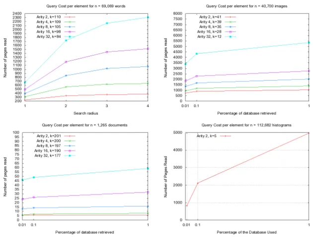
For search experiments, we built the indexes with 90% of the objects and used the other 10% (randomly chosen) as queries. All our results are averaged over 10 index constructions using different database permutations. We have considered range queries retrieving on average 0.01%, 0.1% and 1% of the dataset. This corresponds to radii 0.14, 0.15 and 0.195 for DOCUMENTS, 0.60574, 0.78 and 1.009 for IMAGES, and 0.051768, 0.082514 and 0.131163 for HISTOGRAMS. WORDS have a discrete distance, so we used radii 1 to 4. The same queries were used for all the experiments on the same datasets.
In [2] it was experimentally demonstrated thatDSACL-tree can beat DSA-tree in some of these metric spaces. So, we only show here the behavior of DSACL*-treefor lack of space. As it can be noticed in Figure 1, the maximum arity has a tradeoff with the cluster size, and this tradeoff affects the number of I/O operations performed. If the arity is small, the cluster can increase its size, and it has showed to be good to minimize the I/O operations (see Figure 2). In WORDS the better results is with maximum arity of 2, considering distance evaluations and I/O operations performed during searches. For IMAGES and DOCUMENTS the maximum arity would be 4. In the case of HISTOGRAMS, because the size of each element (112 real numbers are needed to represent each element), the maximum arity allowed is 2.
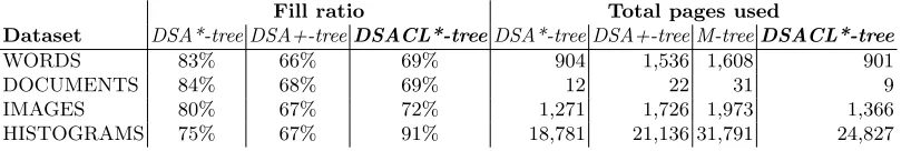
It is also important to notice that our secondary memory version of the DSACL-tree have a good fill ratio, in all cases over 69%. Table 1 shows the average disk page occupancy achieved for the different spaces. In [8] are presented two versions for secondary memory for the DSA-tree (DSA*-tree and DSA+-tree), and the experimental results for them and for theM-tree[4], on the same four metric spaces. We compare the fill ratio and the total number of pages used by these data structures with our results. As it can be noticed we obtain a good fill ratio and we use, in general, fewer disk pages than the other indices designed for secondary memory, while we maintain a good search performance.
7
Conclusions
Fig. 1.Distance evaluations at search time, for the four spaces.
Fill ratio Total pages used
Dataset DSA*-tree DSA+-treeDSACL*-treeDSA*-tree DSA+-tree M-treeDSACL*-tree
WORDS 83% 66% 69% 904 1,536 1,608 901
DOCUMENTS 84% 68% 69% 12 22 31 9
IMAGES 80% 67% 72% 1,271 1,726 1,973 1,366
HISTOGRAMS 75% 67% 91% 18,781 21,136 31,791 24,827
Table 1.Average space usage for the different datasets.
corresponds to a page. By this way, we try to get the most advantage in each read or write into the disk, locating similar objects together. Therefore, we reduce the backtracking at searches improving the cost, in distance evaluations, at the same time we make few I/O operations during the retrieval relevant elements. We have shown some empirical evidence that our new index is competitive considering the space used, with respect to the other dynamic indices for secondary memory such asDSA*-tree, DSA+-treeandM–tree.
For the final version of this paper we plan to include the complete comparison ofDSACL*-treewith the other secondary memory indices.
References
[image:9.612.135.544.400.468.2]Fig. 2.Number of disk pages read at search time, for the four spaces.
Processing and Information Retrieval. pp. 360–368. LNCS 2857, Springer (2003) 2. Barroso, M., Navarro, G., Reyes, N.: Combinando clustering con aproximaci´on
espacial para b´usquedas en espacios m´etricos. In: Actas del XI Congreso Argentino de Ciencias de la Computaci´on. Argentina (2005), in Spanish
3. Ch´avez, E., Navarro, G., Baeza-Yates, R., Marroqu´ın, J.: Searching in metric spaces. ACM Computing Surveys 33(3), 273–321 (Sep 2001)
4. Ciaccia, P., Patella, M., Zezula, P.: M-tree: an efficient access method for similarity search in metric spaces. In: Proc. of the 23rd Conference on Very Large Databases. pp. 426–435 (1997)
5. Hjaltason, G., Samet, H.: Incremental similarity search in multimedia databases. Tech. Rep. CS-TR-4199, University of Maryland, Comp. Science Dept. (2000) 6. Hjaltason, G., Samet, H.: Index-driven similarity search in metric spaces. ACM
Transactions on Database Systems 28(4), 517–580 (2003)
7. Navarro, G., Reyes, N.: Dynamic spatial approximation trees. ACM Journal of Experimental Algorithmics (JEA) 12, article 1.5 (2008), 68 pages
8. Navarro, G., Reyes, N.: Dynamic spatial approximation trees for massive data. In: Proc. 2nd International Workshop on Similarity Search and Applications. pp. 81–88. IEEE CS Press (2009)
9. Samet, H.: Foundations of Multidimensional and Metric Data Structures. Morgan Kaufmann Publishers Inc., San Francisco, CA, USA (2005)