New Deletion Method for Dynamic Spatial
Approximation Trees
Fernando Kasi´an, Ver´onica Ludue˜na, Nora Reyes, and Patricia Roggero
Departamento de Inform´atica, Universidad Nacional de San Luis, San Luis, Argentina
{fkasian,vlud,nreyes,proggero}@unsl.edu.ar
Abstract. The Dynamic Spatial Approximation Tree (DSAT) is a data structure specially designed for searching in metric spaces. It has been shown that it com-pares favorably against alternative data structures in spaces of high dimension
or queries with low selectivity. TheDSATsupports insertion and deletions of
el-ements. However, it has been noted that eliminations degrade the structure over
time. In [8] is proposed a method to handle deletions over theDSAT, which shown
to be superior to the former in the sense that it permits controlling the expected deletion cost as a proportion of the insertion cost.
In this paper we propose and study a new deletion method, based on the deletions strategies presented in [8], which has demonstrated to be better. The outcome is a fully dynamic data structure that can be managed through insertions and deletions over arbitrarily long periods of time without any reorganization.
Keywords: multimedia databases, metric spaces, similarity search
1
Introduction
“Proximity” or “similarity” searching is the problem of looking for objects in a set close enough to a query under a certain (expensive to compute) distance. Similarity search has become a very important operation in applications that deal with unstruc-tured data sources. For example, multimedia databases manage objects without any kind of structure, such as images, fingerprints or audio clips. This has applications in a vast number of fields. Some examples are non–traditional databases, text searching, information retrieval, machine learning and classification, image quantization and com-pression, computational biology, and function prediction. All those applications can be formalized with themetric space model[3]. That is, there is an universeU of ob-jects, and a positive real valued distance functiond: U × U −→ R+
defined among them. This distance may (and ideally does) satisfy the three axioms that make the set a metric space:strict positiveness,symmetry, andtriangle inequality. The smaller the distance between two objects, the more “similar” they are. We have a finite database S ⊆ U, which is a subset of the universe and can be preprocessed. Later, given a new object from the universe (aqueryq), we must retrieve all similar elements found in the database. There are two typical queries of this kind:
Range query: retrieve all elements within distancertoqinS.
The distance is considered expensive to compute. Hence, it is customary to define the complexity of search as the number of distance evaluations performed. We consider the number of distance evaluations instead of the CPU time because the CPU overhead over the number of distance evaluations is negligible in theDSAT. In this paper we are devoted to range queries. In [5] is shown how to build an nearest neighbors algorithm range-optimal using a range algorithm, so we can restrict our attention to range queries. Proximity search algorithms build an indexof the database and perform queries using this index, avoiding the exhaustive search. For general metric spaces, there exist a number of methods to preprocess the database in order to reduce the number of distance evaluations [3]. All those structures work on the basis of discarding elements using the triangle inequality, and most use the classical divide-and-conquer approach. (which is not specific of metric space searching).
The Spatial Approximation Tree (SAT) is a proposed data structure of this kind [6, 7], based on a concept: approach the query spatially. It has been shown that the SAT gives better space-time tradeoffs than the other existing structures on metric spaces of high dimension or queries with low selectivity [7], which is the case in many applica-tions. TheSAT, however, has some important weaknesses: it is relatively costly to build in low dimensions; in low dimensions or for queries with high selectivity (smallrork), its search performance is poor when compared to simpler alternatives; and it is a static data structure: once built, it is hard to add/delete elements to/from it. These weaknesses make theSATunsuitable for important applications such as multimedia databases.
TheDSATis a dynamic version of theSATand overcomes its drawbacks. The dy-namicSATcan be built incrementally (i.e., by successive insertions) at the same cost of its static version, and the search performance is unaffected. At first, theDSAT sup-ports insertion and deletions of elements. However, that deletions degrade the structure over time, so in [8] was presented a deletion algorithm that does not degrade the search performance over time. This algorithm yielded better tradeoffs between search perfor-mance and deletion cost. In this paper we present another alternative method to delete an element of theDSATwhich obtains better costs than methods described in [8].
Full dynamism is not so common in metric data structures [3]. While permitting efficient insertions is quite usual, deletions are rarely handled. In several indexes one can delete some elements, but there are selected elements that cannot be deleted at all. This is particularly problematic in the metric space scenario, where objects could be very large (e.g., images) and deleting them physically may be mandatory. Our algorithms permit deleting any element from aDSAT.
This paper is organized as follows: In Section 2 we give a description of theDSAT. Section 3 presents our new improved deletion method, and Section 4 contains the em-pirical evaluation of our proposal. Finally, in Section 5 we conclude and discuss about possible extensions for our work.
2
Dynamic Spatial Approximation Trees
Algorithm 1Insertion of a new elementxinto aDSATwith roota.
Insert(Node a, Element x) 1. R(a)←max(R(a), d(a, x))
2. c←argminb∈N(a)d(b, x)
3. If d(a, x)< d(c, x)∧ |N(a)|< M axArity Then
4. N(a)←N(a)∪ {x}
5. N(x)← ∅, R(x)←0
6. time(x)←CurrentT ime
7. CurrentT ime←CurrentT ime+ 1
8. Else Insert(c,x)
insertion time of each element is kept. Each nodeain the tree is connected to its chil-dren, which form a set of elements calledN(a), the neighborsofa. When inserting a new elementx, its point of insertion is found by beginning from the tree rootaand pe-rforming the following procedure. The elementxis added toN(a)(as a new leaf node) if (1)xis closer toathan to any elementb∈N(a), and (2) the arity of nodea, |N(a)|, is not already maximal. Otherwisexis forced to choose the closest neighbor in N(a)and keep walking down the tree in a recursive manner, until we reach a nodea such thatxis closer toathan anyb∈N(a)and the arity of nodeais not maximal (this eventually occurs at a tree leaf). At this pointxis added at the end of the listN(a), the current timestamp is put toxand the current timestamp is incremented. The following information is kept in each nodeaof the tree: the set of neighborsN(a), the times-tamptime(a)of the insertion time of the node, and the covering radiusR(a)with the distance betweenaand the farthest element in the subtree ofa.
Note that by reading neighbors from left to right timestamps increase. It also holds that the parent is always older than its children. TheDSATcan be built by starting with a first single nodeawhereN(a) = ∅andR(a) = 0, and then performing successive insertions. Algorithm 1 gives the insertion process.
2.1 Searching
The idea for range searching is to replicate the insertion process of relevant elements. That is, the process act as if it wanted to insertqbut keep in mind that relevant elements may be at distance up torfromq, so in each decision for simulating the insertion ofq a tolerance of±ris permitted, so that it may be that relevant elements were inserted in different children of the current node, and backtracking is necessary.
Two facts have to be considered. The first is that, when an elementxwas inserted, a nodeain its path may not have been chosen as its parent because its arity was already maximal. So, at query time, instead of choosing the closest toxamong{a} ∪N(a), it may have chosen only amongN(a). Hence, the minimization is performed only among elements inN(a). The second fact is that, at the timexwas inserted, elements with higher timestamp were not yet present in the tree, soxcould choose its closest neighbor only among elements older than itself.
Algorithm 2Searching forqwith radiusrin aDSATrooted ata.
RangeSearch(Node a, Query q, Radius r, Timestamp t)
1. If time(a)< t ∧ d(a, q)≤R(a) +r Then
2. If d(a, q)≤r Then Report a
3. dmin← ∞
4. For bi∈N(a) Do /* in ascending timestamp order */
5. If d(bi, q)≤dmin+ 2r Then
6. t′
←min{t} ∪ {time(bj), j > i∧d(bi, q)> d(bj, q) + 2r}
7. RangeSearch(bi,q,r,t′)
8. dmin←min{dmin, d(bi, q)}
timestamp smaller than that of bi+j should be considered when searching insidebi; younger elements have seenbi+jand they cannot be interesting for the search if they are insidebi. As parent nodes are older than their descendants, as soon as a node inside the subtree of bi with timestamp larger than that ofbi+j is found the search in that branch can stop, because all its subtree is even younger.
Algorithm 2 shows the process to perform range searching. Note that, except in the first invocation,d(a, q)is already known from the invoking process.
2.2 Deletions
To delete an elementx, the first step is to find it in the tree. Unlike most classical data structures, doing this is not equivalent to simulating the insertion ofxand seeing where it leads us to in the tree. The reason is that the tree was different at the time xwas inserted. Ifxwere inserted again, it could choose to enter a different path in the tree, which did not exist at the time of its first insertion.
An elegant solution to this problem is to perform a range search with radius zero, that is, a query of the form(x,0). This is reasonably cheap and will lead us to all the places in the tree wherexcould have been inserted.
On the other hand, whether this search is necessary is application dependent. The application could return a handle when an object was inserted into the database, and therefore this search would not be necessary. This handle can contain a pointer to the corresponding tree node. Adding pointers to the parent in the tree would permit to locate the path for free (in terms of distance computations). Hence, in which follows, the location of the object is not considered as part of the deletion problem, although it has shown how to proceed if necessary.
Algorithm 3Deletingxfrom aDSAT, finding a substitute in the leaves of its subtree.
DeleteGH1(Node x) 1. b←parent(x)
2. If N(x)=∅ Then
3. y← FindSubstituteLeaf (x) 4. dg(x)←dg(x) +d(x, y)
5. Copy object of y into node x
6. Else N(b)←N(b)− {x}
FindSubstituteLeaf(Node x): Node
1. y←x
2. While N(y)=∅ Do
3. x←y
4. y←argminc∈N(b)d(c, x)
5. N(x)←N(x)− {y}
6. Return y
delete. This way rebuilding is not necessary, but in exchange some tolerance must be considered when entering the replaced node at search time.
Remind that the neighbors of a nodebin theDSATpartition the space in a Voronoi-like fashion, with hyperplanes. If elementyreplaces a neighborxofb, the hyperplanes will be shifted (slightly, ifyis close tox). We can think of a “ghost” hyperplane, cor-responding to the deleted elementx, and a real one, corresponding to the new element y. The data in the tree is initially organized according to the ghost hyperplane, but in-coming insertions will follow the real hyperplane. A search must be able to find all elements, inserted before or after the deletion ofx.
For this sake, we have to maintain a tolerancedg(x)at each nodex. This is set to dg(x) = 0whenxis first inserted. Whenxis deleted and the content of its node is replaced byy, we will setdg(x) =dg(x) +d(x, y)(the node is still calledxalthough its object is that ofy). Note that successive replacements may shift the hyperplanes in all directions so the new tolerance must be added to previous ones.
At search time, we have to consider that each nodexcan actually be offset bydg(x) when determining whether or not we must enter a subtree. Therefore, we wish to keep dg()values as small as possible, that is, we want to find replacements that are as close as possible to the deleted object. When nodexis deleted, we have to look for a substitute in its subtree to ensure that we reduce the problem size.
Choosing a leaf substitute We descend in the subtree ofxby the children closest tox all the time. When it reach a leafy, it disconnectyfrom the tree and putyinto the node ofx, retaining the original timestamp ofx. Then, thedgvalue of the node is updated.
Choosing a neighbor substitute We selectyas the closest toxamongN(x)and copy objectyinto the node ofxas above. If the former node ofywas a leaf it delete it and finish. Otherwise we recursively continue the process at that node. So, we turn toghost all the nodes in the path fromxto a leaf of its subtree, following the closest neighbors. In exchange, thedg()values should be smaller.
Choosing the nearest-element substitute We selectyas the closest element toxamong all the elements in the subtree ofxand copy objectyinto the node ofxas above. If the former node ofywas a leaf we delete it and finish. Otherwise, we recursively continue the process at that node. Therefore, we turn toghostsome nodes in the path fromxto a leaf of its subtree, following the nearest elements. Thedg()values should be smaller than with the other alternatives.
Algorithm 4Deletingxfrom aDSAT, choosing its replacement among its neighbors.
DeleteGH2(Node x) 1. b←parent(x)
2. If N(x)=∅ Then
3. y←argminc∈N(x)d(c, x), dg(x)←dg(x) +d(x, y)
4. Copy object of y into node x
5. DeleteGH2 (y)
6. Else N(b)←N(b)− {x}
Algorithm 5Deletingxfrom aDSAT, choosing its replacement as its nearest element.
DeleteGH3(Node x) 1. b←parent(x)
2. If N(x)=∅ Then
3. y← NNsearch(x,x,1), dg(x)←dg(x) +d(x, y)
4. Copy object of y into node x
5. DeleteGH3 (y)
6. Else N(b)←N(b)− {x}
Thus, for a permanent regime that includes deletions, we must periodically get rid of ghost hyperplanes and reconstruct the tree to delete them. Just as with fake nodes [8], when we rebuild the subtree we get rid of all the ghost hyperplanes that are inside it. We set a maximum allowable proportionαof ghost hyperplanes, and rebuild the tree when this limit is exceeded.
3
A New Deletion Method
In [8] it is concluded that the methods with the best performance during deletions use ghosts hyperplanes. Moreover, these methods have the possibility of using the param-eterαto control the deletion average cost. Our new proposal to delete an elementxis based on the best strategies presented in [8]. Therefore, this new proposed method is also based on the idea presented in [10], which useghost hyperplanes.
We believe that the way to achieve a good tradeoff between the number of hy-perplanes and the displacement of eachdf can be obtained by replacing the deleted elementxwith the leaf of his subtree whose distance is minimal; i. e.the closest leaf in the complete subtree ofx. Therefore, with each deletion only one new ghost hyperplane appears and the displacement of this ghost hyperplane, although it is not necessarily the smallest one possible, is expected to be fairly close to it.
Algorithm 6Deletingxfrom aDSAT, finding a substitute as theclosest leaf.
DeleteGH4(Node x) 1. b←parent(x)
2. If N(x)=∅ Then
3. y← FindSubstituteNNLeaf(x) 4. df(x)←df(x) +d(x, y)
5. Copy object of y into node x
6. Else N(b)←N(b)− {x}
FindSubstituteNNLeaf(Node x): Node
1. Q← ∅, L← ∅
2. For v∈N(x)
3. If N(v) = 0 Then L← {(v, x)}
4. Else Q← {v}
5. While Q not empty
6. b ← first element of Q, Q ← Q− {b}
7. For v∈N(b)
8. If N(v) = 0 Then L←L∪ {(v, b)}
9. Else Q ← Q ∪ {v}
10. (y, v)←argmin(z,t)∈Ld(x, z), N(v)←N(v)− {y}
11. Return y
in level-order. Finally, when the full set of leaves of the subtree ofxis determined, we select the leafy that satisfies:d(x, y)< d(x, z),∀(z, t)∈ L− {(y, v)}, thenyis returned after it is disconnected from its father.
This new method is based on the idea to obtain a better deletion strategy by consid-ering the best characteristics of GH1 and GH3: only one ghost hyperplane appears after each deletion, and its displacement is nearby to the possible best one. Clearly, we can also set a maximum allowable proportionαof ghost hyperplanes, and rebuild the tree when this limit is exceeded.
4
Experimental Results
As it is aforementioned, we do not consider the cost to locate the element as part of the deletion problem, then the deletion costs obtained represent only the necessary work to effectively delete the element from theDSAT. Thus, we can directly compare our experimental results with those presented in [8]. To study the behavior and performance of this new deletion algorithm forDSAT, we need to evaluate the proper deletion costs and also the searching performance after that.
In order to make a fairly comparison between the previous deletion methods and the new one, we use the same metric spaces considered in [8] to evaluate the performance ofDSAT, available from [4]. We use the best arity for each space, as it is described in [8]. They are four real-life metric spaces with widely different histograms of distances:
NASA images:a set of 40,700 20-dimensional feature vectors, generated from images downloaded from NASA.1The Euclidean distance is used.
Color histograms: a set of 112,682 8-D color histograms (112-dimensional vectors) from an image database.2Any quadratic form can be used as a distance, so we chose Euclidean distance.
Documents:a set of 1,265 documents under the Cosine similarity, heavily used in In-formation Retrieval [1]. In this model the space has one coordinate per term and doc-uments are seen as vectors in this high dimensional space. The distance we use is the angle among the vectors. The documents are the files of theTREC-3 collection.3
There are two types of experiments:
1. We build the index with the 90% of the database elements, the other 10% is used as queries for range searches. After the index is built, we delete a 10% of elements randomly selected.
2. We use the 60%, 70%, 80%, and 90% of the database elements to build the index. Then we delete the 10%, 20%, 30%, and 40% respectively, in order to leave 50% of the elements into the tree in each index. It can be noticed that in each case the 50% of the database, that remains after deletions into the tree, is not necessarily the same set of elements, as the elements deleted are randomly selected. Then, we perform queries with the non-inserted 10% of database elements.
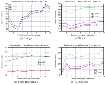
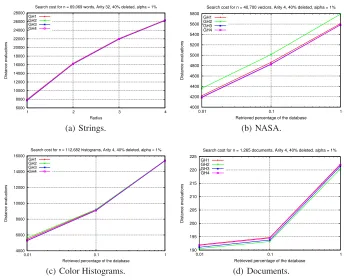
We have tested several options in our experiments. For the parameterαwe con-sider: 0% (without any ghost hyperplane), 1%, 3%, 10%, 30%, and 100% (without any rebuilding). In all cases, ifα= 0%, as is pure rebuilding, costs are higher. Then, as the proportionαof allowed ghost hyperplanes grows, deletion costs decrease. For range search we consider three radii for the spaces with continuous distance, and four radii for Strings space (with discrete distance). For lack of space we only show some ex-amples: for the first type of experiment, the comparison of deletion costs forα= 1% when the 10% of elements is deleted; for the second one, the comparison of search costs obtained after 40% of elements is deleted withα= 1%, considering the 10% of reserved elements as queries. Figure 1 shows, for the first type of experiment, the aver-age deletion costs obtained per element when 10% of the elements is deleted. Figure 2 illustrates, for the second type of experiment, the average search costs per element, after 40% of the database is deleted usingα= 1%, when we search with the reserved 10% of elements as queries. As it can be noticed, our deletion method (GH4) obtains very good performance, both in deletion and search costs, for all metric spaces considered.
5
Conclusions
We have designed a new algorithm for efficient deletion inDSAT. This new algorithm has a low cost of deletion and allows that subsequent searches have a performance similar to the best algorithm proposed in [8]. On the other hand, efficient searches are still maintained: it is possible to apply the same algorithms ofDSAT for range search andkclosest neighbors. Our deletion algorithm kept, as a parameter, the proportion of
1
Athttp://www.dimacs.rutgers.edu/Challenges/Sixth/software.html 2At
http://www.dbs.informatik.uni-muenchen.de/˜seidl/DATA/histo112.112682.gz 3
allowed nodes with ghost hyperplanes in the tree, which permits us to tune search cost versus deletion cost.
The outcome is a much more practical data structure that can be useful in a wide range of applications. We expect theDSAT, with the new deletion algorithm, to replace the static version in the developments to come.
As future work we plan to add our new deletion algorithm to the existing version ofDSAT for secondary memory [9], since it has the advantage that only one ghost hyperplane is created, so only two nodes have to be changed, for each deletion. In this case will be relevant both number of distance evaluations and number of I/O operations.
1100 1150 1200 1250 1300 1350 1400 1450 1500 1550 1600 1650
1 2 3 4 5 6 7 8 9 10
Distance evaluations
Deleted percentage of the dataabase Deletion cost for n = 69,069 words, Arity 32, alpha = 1%
GH1 GH2 GH3 GH4 (a) Strings. 160 170 180 190 200 210 220 230 240 250 260
1 2 3 4 5 6 7 8 9 10
Distance evaluations
Deleted percentage of the database Deletion cost for n = 40,700 vectors, Arity 4, alpha = 1%
GH1 GH2 GH3 GH4 (b) NASA. 100 150 200 250 300 350 400
1 2 3 4 5 6 7 8 9 10
Distance evaluations
Deleted percentage of the database Deletion cost for n = 112,682 histograms, Arity 4, alpha = 1%
GH1 GH2 GH3 GH4
(c) Color Histograms.
100 150 200 250 300 350
1 2 3 4 5 6 7 8 9 10
Distance evaluations
Deleted percentage of the database Deletion cost for n = 1,265 documents, Arity 4, alpha = 1%
GH1 GH2 GH3 GH4
[image:9.595.133.477.253.532.2](d) Documents.
Fig. 1.Comparison of deletion costs, for all deletion algorithms usingα= 1%.
References
1. R. Baeza-Yates and B. Ribeiro-Neto.Modern Information Retrieval. Addison-Wesley, 1999.
2. S. Brin. Near neighbor search in large metric spaces. InProc. 21st Conference on Very Large
Databases (VLDB’95), pages 574–584, 1995.
3. E. Ch´avez, G. Navarro, R. Baeza-Yates, and J. Marroqu´ın. Searching in metric spaces.ACM
4. K. Figueroa, G. Navarro, and E. Ch´avez. Metric spaces library, 2007. Available at
http://www.sisap.org/Metric Space Library.html.
5. G. Hjaltason and H. Samet. Incremental similarity search in multimedia databases. Technical Report CS-TR-4199, University of Maryland, Computer Science Department, 2000.
6. G. Navarro. Searching in metric spaces by spatial approximation. InProc. String Processing
and Information Retrieval (SPIRE’99), pages 141–148. IEEE CS Press, 1999.
7. G. Navarro. Searching in metric spaces by spatial approximation.The Very Large Databases
Journal (VLDBJ), 11(1):28–46, 2002.
8. G. Navarro and N. Reyes. Dynamic spatial approximation trees. ACM Journal of
Experi-mental Algorithmics (JEA), 12:article 1.5, 2008. 68 pages.
9. G. Navarro and N. Reyes. Dynamic spatial approximation trees for massive data. In T. Skopal
and P. Zezula, editors,SISAP, pages 81–88. IEEE Computer Society, 2009.
10. R. Uribe and G. Navarro. Una estructura din´amica para b´usqueda en espacios m´etricos. InActas del XI Encuentro Chileno de Computaci´on, Jornadas Chilenas de Computaci´on, Chill´an, Chile, 2003. In Spanish. In CD-ROM.
6000 8000 10000 12000 14000 16000 18000 20000 22000 24000 26000 28000
1 2 3 4
Distance evaluations
Radius
Search cost for n = 69,069 words, Arity 32, 40% deleted, alpha = 1%
GH1 GH2 GH3 GH4 (a) Strings. 4000 4200 4400 4600 4800 5000 5200 5400 5600 5800
0.01 0.1 1
Distance evaluations
Retrieved percentage of the database Search cost for n = 40,700 vectors, Arity 4, 40% deleted, alpha = 1%
GH1 GH2 GH3 GH4 (b) NASA. 4000 6000 8000 10000 12000 14000 16000
0.01 0.1 1
Distance evaluations
Retrieved percentage of the database Search cost for n = 112,682 histograms, Arity 4, 40% deleted, alpha = 1%
GH1 GH2 GH3 GH4
(c) Color Histograms.
190 195 200 205 210 215 220 225
0.01 0.1 1
Distance evaluations
Retrieved percentage of the database Search cost for n = 1,265 documents, Arity 4, 40% deleted, alpha = 1%
GH1 GH2 GH3 GH4
[image:10.595.133.477.319.599.2](d) Documents.