ON-SITE MEASUREMENTS VERSUS ANALYTICAL APPROACH IN THE
ELABORATION OF NOISE MAPS AND ASSESSMENT OF THE CRITICAL
FACTORS
PACS: 43.50.Sr
Manuela Almeida 1; Luís Bragança 1 and Manuela Nogueira 2
1
University of Minho;
Civil Engineering Department, Azurém 4800-058 Guimarães, Portugal
E-mail: malmeida@civil.uminho.pt; braganca@civil.uminho.pt
2
Municipality of Guimarães, Portugal E-mail: nogueira56@hotmail.com
ABSTRACT
Recent European guidelines, as well as national legislation, make mandatory the elaboration of strategic noise maps for residential areas every five-year for cities with more than 250 000 inhabitants. These maps will help to determine and quantify in what way people are annoyed and disturbed by the surrounding noise. However, there are no European standards for the determination of outdoor noise. Each country is responsible for the definition of its own evaluation methods. But, in some situations, the available methods can lead to great differences in the resulting sound levels that can go up to 10 dB(A). Due to very recent legislation, Portugal is now giving the first steps in producing noise maps. Some difficulties in choosing the noise evaluation methodology are arising with some technicians using only analytical prevision methods and others preferring the experimental and field evaluation of noise. The aim of this work is to evaluate the accuracy and versatility of a common prevision method by comparing the results obtained by simulation with those obtained with on-site measurements. It is also a goal of this paper to enlighten the critical points where and when the majors differences between these two methodologies occur.
RESUMO
afectam a precisão dos métodos utilizados, a partir dos quais surgem as maiores diferenças entre estas duas metodologias.
1. INTRODUCTION
Noise has become one of the most important degradation factors of people’s quality of life. Human being, especially in urban areas, lives surrounded by noise, which causes discomfort and stress and is responsible for a great number of psychological and physical damages. The ever-growing technological development of our cities has been leading to a continuous increase in the sound levels observed in urban areas caused, essentially by traffic and industries.
To prevent critical health effects, World Health Organization in 1996 suggested the value of 55 dB(A) for the A-weighted equivalent outdoor sound level, LAeq, during the day (the equivalent
sound level is the average sound level during a certain period of time which means that short peaks in the sound level only have a slight influence on LAeq). To reinforce this intention, the 5
th
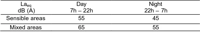
European Action Program related to the Environment has also defined some specific objectives to be achieved in terms of noise reduction: all equivalent sound levels above 55 dB(A) should be gradually reduced to values between 55 and 65 dB(A) and in any circumstance they should be greater than 85 dB(A). Recent Portuguese legislation [1] is more ambitious establishing the difference between sensible areas and mixed areas and between day period and night period imposing different noise level limits for each situation as it can be seen in table 1.
[image:2.596.130.463.404.458.2]To achieve these results, extensive elaboration of noise maps throughout European urban areas is essential in order to identify the problematic areas. These maps will be useful tools for improving the noise situation of existing and future residential areas.
Table 1: Maximum outdoor noise level
Laeq
dB (A)
Day 7h – 22h
Night 22h – 7h
Sensible areas 55 45
Mixed areas 65 55
According to very recent European directives [2], all urban areas with more than 250º000 inhabitants and areas near important roads (with more than 6 millions of vehicles per year), railways (with more than 60 000 trains per year) and airports (with more than 50 000 flights per year), must produce noise maps till July 2007. After that, the same action will have to be carried out for cities with 100 000 inhabitants, roads with more than 3 millions of vehicles per year and railways with more than 30 000 trains per year in order to reduce the number of people disturbed. This is absolutely in line with recent Portuguese legislation [1]. However, some difficulties have arisen in the application of this legislation mostly because the technicians don't know the law well and when they are aware of it, it is sometimes ambiguous and difficult to apply.
In spite of recent publications by the Portuguese Ministry of Economy [3,4] defining some guidelines for noise map elaboration, there are no Portuguese standards in the field unless the NP-1730-2 standard [5] that defines the methodology to be followed in the graphical representation of the results. This lack of official methodologies and procedures has been leading to some anarchy and many doubts are arising in the elaboration of the maps. The guidelines define the parameters that have to be taken into account but the methodology to be followed depends on the technician choice. Some prefer using prevision methods while others prefer on-site measurements campaigns. Since there is no experience in this field, this work tried to compare these two approaches. The aim was to compare the results obtained with both methodologies trying to identify what are the differences and when and why they occur. For this purpose, part of the city of Guimarães has been chosen.
To compare the two methodologies, the outdoor noise in the selected zone has been evaluated by on-site measurements and by simulation. The results have been compared and the differences between them have been assessed. The most relevant parameters that have a major interference on the noise map definition have also been identified.
2.1. Prevision Method
Among those available, the simulation code chosen to predict the noise levels was MITHRA [6] because it is one of the most popular codes used in Portugal. This software follows a model that takes into account the buildings’ geometry and type of façade, local topography, properties of the ground, meteorological conditions and the existence of acoustical barriers. In spite of all the potentialities of MITHRA, only road traffic has been considered in this study not only because it has a dominant role but specially because in the selected area there isn’t any airport, railway or important industry. In this case, the sound levels depend on the traffic intensity, percentage of heavy traffic, average speed of the vehicles, characteristics of the road pavement, acoustical properties of the ground between road and receiver, distance between road and receiver and height of the buildings and type of their coating.
To obtain all these data, this methodology also implies an on-site campaign to determine or to confirm the physical characteristics of the zone since in most of the cases this information (or at least part of it) is not available. It is also important to locally identify the presence of any walls or acoustical barriers, the presence of any woods or parks and of any lakes or rivers since they have an important role on the definition of the local noise levels.
Traffic counting is also a very important input of the program with great influence on the final results. In this study, some of these values were available (main roads) but others were not. In this case, the missing values were extrapolated based on the existing ones or they were measured. When they were measured, these measuring campaigns were performed for periods of one hour each.
This model is based on a fast algorithm, particularly adapted to road traffic, that identifies the acoustical paths between the sound source and the receiver taking into account direct, refracted and reflected (by the ground and by the buildings façades) sound beams.
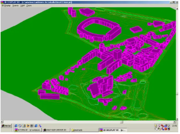
2.2. Selected Area
Figure 1. Zone selected to perform the study
2.3. On-site Measurements
The results obtained by simulation had to be compared with the noise levels observed in-situ. For this purpose, twelve representative points of the zone under study have been selected and a one-month measurement campaign has been performed. The selected points were representative of the most problematic sites in the city in terms of noise.
The sound levels measurements took place in the evening between 18h and 20h, in a rush hour period. This decision was based on a deep knowledge of the city habits otherwise it would have been necessary to perform the measurements in a larger period and to repeat them at different hours in order to characterize the zone. The measurements period had also to be coincident with the period for what traffic counting was available in order that a correct comparison between the two methodologies could be done. In each receiver, the measurement period corresponded to fifteen minutes repeated twice. The choice of such a short period was due to the uniformity of the existent outdoor noise at the time of the measurements.
3. OUTDOOR NOISE EVALUATION
The outdoor noise levels in the selected area of the city of Guimarães were determined by simulation and by on-site measurements. The A-weighted equivalent outdoor sound levels, LAeq, obtained in the twelve receiver points, were afterwards compared and the results of this
[image:4.596.144.453.69.299.2]0 10 20 30 40 50 60 70 80 90
1 2 3 4 5 6 7 8 9 10 11 12
receiver number
Leq dB(A)
measured simulated
Figure 2. Comparison between measured and simulated LAeq values
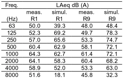
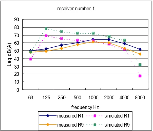
In average, this figure shows that the differences between the simulated values and the measured ones vary from to 2 to 3 dB (A). However, there are four points that are clearly off of this range: receivers 2, 6, 7 and 9. In these cases, the differences between the measured and the simulated values are, respectively, 4.8 dB (A), 6.2 dB (A), 7.6 dB (A) and 10.6ºdB (A), which are too high values and therefore not acceptable. Figure 3 and table 2 show the noise spectrum in two of these points (1 and 9).
[image:5.596.153.443.71.242.2]The analysis of this situation allowed concluding that these major differences were due to a discrepancy between the traffic counting introduced in the program and the effective number of vehicles passing in the roads at the time of the measurements. In the simulations it was used an available official counting which was different from the values observed in situ during the noise levels measurements. It was also noticed a discrepancy in the percentage of heavy traffic used in the simulations and the one observed in situ. Another important aspect was related to the fact that the measurements were performed at 1.5 m above the ground level while the simulation results were produced for a receiver located 5 m above the ground. It is important to note that the lack of rigor in introducing the site characteristics led to differences between the measured and the simulated values up to 10 dB (A), which enhances the great importance of the accuracy of the data introduced in the model.
Table 2: Noise levels/octave in two points
Freq. LAeq dB (A)
(Hz)
meas. R1
simul. R1
meas. R9
simul. R9
63 50.0 39.3 48.0 48.4
125 52.3 69.2 49.7 78.3
250 57.0 65.6 53.3 74.7
500 60.4 62.9 58.1 72.1
1000 64.3 62.7 61.4 72.1
2000 64.1 58.3 60.4 68.2
4000 58.9 52.0 53.3 63.0
[image:5.596.192.402.518.653.2]receiver number 1
0 10 20 30 40 50 60 70 80 90
63 125 250 500 1000 2000 4000 8000
frequency Hz
Leq dB(A)
measured R1 simulated R1
[image:6.596.170.415.74.283.2]measured R9 simulated R9
Figure 3. Comparison between measured and simulated LAeq values
The analysis of this situation allowed concluding that these major differences were due to a discrepancy between the traffic counting introduced in the program and the effective number of vehicles passing in the roads at the time of the measurements. In the simulations it was used an available official counting which was different from the values observed in situ during the noise levels measurements. It was also noticed a discrepancy in the percentage of heavy traffic used in the simulations and the one observed in situ. Another important aspect was related to the fact that the measurements were performed at 1.5 m above the ground level while the simulation results were produced for a receiver located 5 m above the ground. It is important to note that the lack of rigor in introducing the site characteristics led to differences between the measured and the simulated values up to 10 dB (A), which enhances the great importance of the accuracy of the data introduced in the model.
Besides these three parameters (number of vehicles, percentage of heavy traffic and height of the measuring point), there are also others that have a great influence on the results obtained by simulation like the velocity of the vehicles, type of road pavement, buildings height, type of coating of the façades or width of the road.
Some sensitivity studies have been performed in order to evaluate the interference of these parameters on the accuracy of the simulated noise levels. The intention was to identify the parameters with what technicians must take special care.
From those studies it became evident that the velocity, percentage of heavy traffic and number of vehicles per hour on the road were the most relevant.
When the velocity of the vehicles was changed in 20% (either up or down), through the simulations it was observed that the LAeq values changed in about 3 dB (A) with a minimum value observed of 0.9 dB and a maximum of 8.3 dB (A) depending on the site characteristics.
Changing the number of vehicles in 30% it would lead to an increase (or decrease) of 2 dB (A) on the LAeq values. However, depending on the site characteristics, it has also been observed increases of more than 8 dB (A) on the LAeq values.
4. CONCLUSIONS
been compared: one using a simulation code to predict the A-weighted equivalent outdoor sound levels of part of the city of Guimarães and other measuring in-situ these sound levels.
The comparison of both results showed that in the majority of the cases, the simulated values were close to the measured ones with differences between them that varied from 1 to 3 dB (A). However, it became evident that the accuracy of the data used in the simulation code is of high importance since it has been observed differences that went up to 10 dB (A) between the simulated and the measured values when there was a discrepancy between the input data of the code and the real situation.
Sensitivity studies showed that the most relevant parameters that have a major interference on the accuracy of the final results are the number of vehicles per hour in each road, their velocity and the percentage of heavy traffic present. When variations of about 20% to 30% on these parameters occur, the LAeq values vary in about 3 dB (A) but the increases (or decreases) observed can also go up to more than 8 dB (A).
Also the width of the roads, type of pavement, shape of the buildings and their coating cannot be neglected in all the process.
The major conclusion of this work is that unless we are certain of the accuracy of the available data, it is wise to follow a mixed methodology where prevision methods are complemented with field measurements in order to produce rigorous noise maps in accordance with reality.
REFERENCES
1. Regime Legal da Poluição Sonora. Decreto-Lei n.º 292/2000, Lisboa , Novembro 2000. 2. European Parliament, Directive 2002/49/CE – Environmental noise assessment. June
2002.
3. “Elaboração de mapas de ruído – Princípios orientadores”, Direcção Geral do Ambiente, Lisboa, Outubro de 2001.
4. “Recomendações para selecção de métodos de cálculo a utilizar na previsão de níveis sonoros”, Direcção Geral do Ambiente, Lisboa, Setembro de 2001.
5. Norma Portuguesa - NP 1730 – Descrição e medição do ruído ambiente. Lisboa, 1996. 6. MITHRA – Environmental noise prediction software, 0,1 dB-Stell, MVI Technologies