ANALYTICAL MODEL OF LIGHTWEIGHT FLOOR SIMULATION

(1)

ANALYTICAL MODEL OF LIGHTWEIGHT FLOOR SIMULATION

PACS REFERENCE: 43.50.Pn, 43.40.Dx

M. S. Kartous

Engineering Acoustics, LTH, Lund University and

Acoustic section of SP, Swedish National Testing and Research Institute Box 857

SE-50115 Borås Sweden

Tel: +46-33-165439 Fax: +46-33-138381

E-mail: mark.kartous@sp.se

ABSTRACT

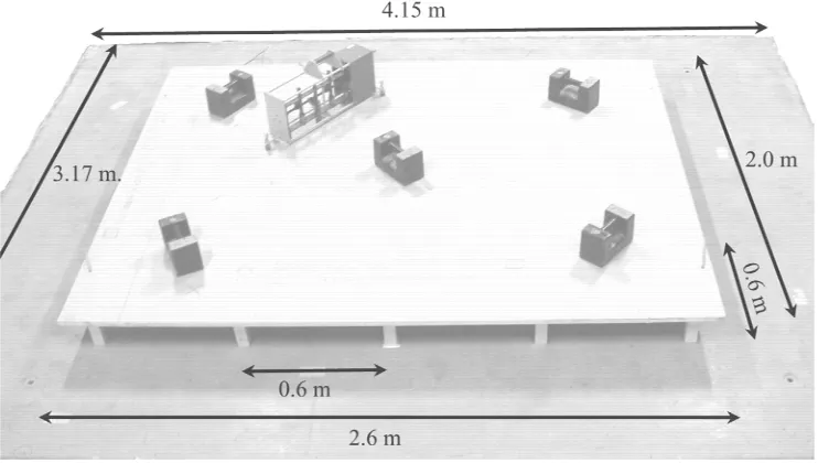
[image:1.595.112.483.521.731.2]

A theoretical model of a construction addition on top of the concrete slab, used for impact sound measurements, substituting a full-scale lightweight floor in a laboratory floor opening is presented. This new test method makes it possible to extend impact sound improvement according to ISO 140-8 to be valid also for lightweight floors. The experimental part of this project has been conducted earlier and resulted in good agreement in comparison of impact sound insulation improvement between a lightweight wooden floor and simulation of the new method. The part described in this paper shall lead to an analytical lumped model of the measurement set-up and method, since some parts of the results and acoustic behaviour of the floor could not be optimised or explained satisfactory.

(2)

INTRODUCTION

A simple impact test procedure for lightweight floors that could be carried out without floor exchange has been proposed by Nordtest and developed empirically. The procedure involves a small lightweight construction placed on top of the standard concrete floor, which can be easily mounted by two persons in about half an hour. Tests that have been carried out on this test floor were compared with laboratory measurements on a complete lightweight joist floor with promising results. The cost of the test rig, total man-time spent and the small area of the test specimen make the method very interesting. In this paper the method is analysed theoretically. The lumped model is divided into a tapping machine, a free-free chipboard plate, here also called the top floor, loaded with five 25 kg weights, supported with twenty wooden legs and standing on a free-supported concrete plate. The modelled legs can easily be connected in series, so other materials in layers can be calculated. The contribution in parallel i.e. the air volume in the cavity between the two plates is to be added to the model in the future.

[image:2.595.87.350.550.728.2]

The model can easily be used for other construction types or purposes. Like floors on adjustable feet and under some circumstances even for joist floors. The influence of loading and combinations of materials in the top-floor layer can also be studied. The set-up of the top floor, the legs, the concrete slab, the five loading weights and the tapping machine is clearly visible in figure 1. The analysis is made under the assumption that the linear Kirchhoff’s plate theory is valid and the amplitudes are small. The time function

e

i tw is omitted.

TAPPING MACHINE MODEL

The standard ISO tapping machine is modelled as a point acting Dirac-source. Since the frequency of the tapping machine is 10 Hz and the acoustic frequency of interest ranges from 50 to 3150 Hz, the contributing energy has to be divided into 10 Hz steps from the third-octave lower frequency limit 44.7 Hz, to the third-octave upper frequency limit 3550 Hz. All-in-all 350 discrete steps. Each third-octave band consists hereby of the frequencies that fall within the band limits. [1] The force from tapping machine impact is expressed in eq. (1).

(

, ,

, , ,

0 T

)

under over, T

F

w

K M R v f

=

F

f

(1)

The Fourier impacts transforms of a single impact can be seen in eq. (4) the over-critical or stuck-to-the-floor case and eq. (5) the under-critical or rebound case. The choice of over- or under-critical case in eq. (1) is dependant of if

W

(4) is real. Then the over-critical case (2) is used, or else the under-critical case (3) is used.

oc

0 2 over

v KM

F

i KM

K

M

R

w

=

-

+

(2)

2

0

2

1

uc

K i

R under

e

F

v KM

i KM

K

M

R

p _w

w

æ ö - _ç + _÷ W è ø

+

=

-

+

(3)

(

)

2

oc

K R

K M

W º

-

(4)

(

)

2

uc

K M

K R

W º

-

(5)

(3)

falling hammer before impact 0.886 [m/s]; w = frequency of interest; F = excitation force; m’’= chipboard mass per unit area:

L

_x

or

l

_xis in direction of x-axis

L

_y

or

l

_yis in direction of y-axis;

w = frequency; wpq = eigenfrequency; v = velocity; p = excitation pressure; x,y = positions on

chipboard (x’,y’ excitation; x,y reception).

LUMPED PLATE MODEL

The assumption made in the modelled plate is that there only exist bending waves and that the thickness is much smaller then the other dimensions. The supports, loading mass and tapping hammer are assumed to act as points. The finite plate has the general two-dimensional equation of motion [3,4]:

( )

_,

2

( )

_,

(

v x y

m

¢¢

w

v x y

j p x y

w

DD

-

=

,

)

(6)

where

_{D = ¶ ¶ + ¶ ¶}

2

_x

2 2

_y

2

The equation (6) has solution for zero excitation

p x y

( )

,

=

0

and eigenfrequencies

j

_pq and eigenfunctions

w

_pq.

DD

j

_pq

( )

x y

,

-

m

¢¢

w

_pq2

j

_pq

( )

x y

,

=

0

(7)

The velocity of a receiving point on the plate compared to an excitation point on the same plate:

(

)

(

2

) ( )

2

(

)

1 1

,

4 ,

,

pq pq

,

p q

x y pq

x y

Fj

v x y x y

FG x y x y

m l l

j

w

¥ ¥

= =

¢ ¢

=

¢ ¢

¢¢

åå

-

(8)

The Green function for a rectangular simply supported plate:

(

)

(

2

) ( )

2 1 1

,

4 ,

,

pq pq

p q

x y pq

x y

x

j

x y x y

m l l

j

w

¥ ¥

= =

¢ ¢

=

¢¢

åå

-n

G

y

(9)

The concrete floor is modelled as an edge supported plate. From the boundary conditions for the eigenequation is given by (10) and the eigenfrequency by (11).

( )

,

sin

pq

x y

p x

q

x y

l

p

j

=

y

(10)

( )

2 2

pq x y

x y

B

p

q

B

k

m

l

m

p

w

=

¢

_¢¢

é

_ê

ê

æ

ç

ö

÷

+

æ

ç

_ç

_÷

ö

÷

_ú

ú

ù

=

_¢¢

¢ é

_ê

_ë

+

_ú

ù

_û

è

_{ø è}

ø

ë

û

(11)

The top floor is modelled as a free-free supported plate. A simplification is used when creating a plate from the product of two free-free supported bars into two-dimensional space. This simplification is still better than using the product of two guided beams. In comparison the peek-offset created by heavy curvature near the ends, leading to zero angle contributes to inferiority of the guided beams solution. [2,4]

The Green function is the same as for the freely supported plate, but the eigenequation is changed into:

( )

,

cos

cosh

sin

sinh

pq x

x x x x

pkx

x y

A

l

j

=

é

ê

æ

ç

+

ö æ

÷ ç

+

ù

ú

ê

è

ø è

ú

ë

û

(4)

… _y

cos

cosh

sin

sinh

y y y y

pkx

A

l

é

æ

ö æ

ù

+

ê

ç

_ç

÷ ç

_{÷ ç}

ú

ê

_è

_{ø è}

ú

ë

û

ö

÷÷

ø

(

g

;

)

(

)

cos

cosh

sin

sinh

kl

A

kl

-=

+

(12)

WOODEN LEGS MODEL

The wooden-feet are modelled as twenty two-port or four-pole couplings between top-floor and concrete floor. This is done under the assumption that the transfer through the leg is in the form of quasi-longitudinal waves and that the bending moment is negligible since the leg is not rigidly connected to the concrete plate but only standing freely on the same. [3]

(

)

(

)

(

)

(

)

cos

sin

1 sin

cos

Ln n Ln Ln n

Ln n Ln n

Ln

k h

jZ

k h

j

k h

Z

é

ù

ê

ú

= ê

ú

ê

ú

ë

û

n

Z

(13)

Area S << bending wavelength in plate 1/6 of bending wavelength in plate, (14) is the longitudinal wave impedance, and (15) the wavenumber of quasi-longitudinal waves.

Fn,vn

S

m

ES

Z

_Ln

=

¢

(14)

ES

m

k

_Ln

=

w

¢

(15)

Fn0,vn0

Figure 2

ESTABLISHMENT OF THE G-MATRIX AND THE GLOBAL SOLUTION

The velocity in an arbitrary point without other points is expressed as the zero fields.

The reactive field, consisting of other forces like the support-legs and the loading mass, also influences resulting velocity in arbitrary point with other points present.

0

F

=

0

v G

0

F

_{R R}

=

0

-v G

G F

(16)

The matrix of reactive forces is not known. The displacement of supports is first set to zero to find the and thereafter used to obtain v. Point support generates v = 0 in the support and hereby two equations and two unknowns.

R

F

n0 n

F

v

n

é

ù

é ù

₌

ê

ú

ê ú

ë û

Z

ë

û

(17)

where

Z

_nis the impedance of the leg. See figure 2.

Let

v

_n0

=

0

i.e. no motion in the lower point in figure 2. This yields

n n

F

B

=

Þ

ú

û

ù

ê

ë

é

=

ú

û

ù

ê

ë

é

n n0

n n

v

0 F

v

F

n

(5)

0

F

_{R R}

=

0

-BF G

G F

Þ

BF GF F G

+

=

0 0

Û

[

B G F F G

+

]

=

0 0

Þ

F

_R

=

F G B G

0 0

[

+

]

-1

By inserting

F

_R into (16) we yield the velocity. Inserting

F

_R and v into

ntop nc 1 ntop nc

F

v

n

-é

ù

é ù

=

_ê

ê ú

ë û

Z

ë

û

ú

(19)

we yield and on top of the concrete slab. used together with the

G

for the free-supported concrete plate in an arbitrary point.

nc

F

v

_nc

F

_nc _c

c

F

=

c c

v

G

Loading mass, the five 25 kg weights, generates an extra matrix of Green functions that is added to the reactive field matrix.

G

_ij

=

(

x

_i

¢ ¢

,

y x y

_i _j

,

_j

)

in eq. (20) and (21).

1 01 11 12 1

2 02 21 22

0 0 1

G

F

G

F

G

F

n

n n n nn

v

G

v

G

F

v

G

é ù

é

ù é

ù é ù

ê ú

ê

ú ê

ú ê ú

ê ú

ê

ú ê

ú ê ú

=

_{ê ú}

=

_ê

_{ú ê}

-

_{ú ê ú}

ê ú

ê

ú ê

ú ê ú

ê ú

ê

ú ê

ú ê ú

ë û

ë

û ë

û ë û

v

L

M

O

L

1 2 n

M

F

G

ù é ù

ú ê ú

û ë û

M

(20)

Where the forces to the outmost right can be from support legs or mass loads.

1 1 01 11 12 1 1

2 2 02 21 22 2

0

0 1

0

0 F

G

0 F

G

0

0 F

G

n

n n n n nn n

B

G

B

G

F

B

G

é

ù é ù

é

ù é

ê

ú ê ú

ê

ú ê

ê

ú ê ú

₌

ê

ú ê

-ê

ú ê ú

ê

ú ê

ê

ú ê ú

ê

ú ê

ê

ú ê ú

ê

ú ê

ë

û ë û

ë

û ë

L

M

O

M

O

L

(21)

By solving

F

₁

,

F

₂

K

F

_n and inserting into eq. (20) we yield v for the points under the top-plate. By using the impedance function for the wooden legs (17) and

v

_ntopand

F

_ntop, we yield

v

_ncand

nc

F

for the contact points on top of concrete plate.

1top 2top ntop

1c 2c nc 1

1top 2top ntop 1c 2c nc

F

v

n

-

é

ù

é

ù

₌

ê

ú

ë

û

Z

ë

û

L

ú

1 1 c c

ù

ú

úû

M

)

,

(22)

New free-field G matrix is established since the concrete plate has other dimensions, material properties and is free supported along the edge.

v

_nc

=

G F

₀_nc ₀_nc

1 11 12 1

2 21 22

1

c c c nc

c c c

c

nc n c nnc nc

v

G

F

v

G

F

v

G

F

é ù é

ù é

ê ú ê

ú ê

ê ú ê

ú ê

=

_{ê ú ê}

=

_{ú ê}

ê ú ê

ú ê

ê ú ê

ú ê

ë û ë

û ë

v

L

M

O

L

(23)

Velocity in an arbitrary contact point on the concrete plate can be generally expressed as

( )

_{( )}

₍

1 1 1 1 , 1

ˆ

,

pq N N n

c n n n pq pq pq pq

n p q n p q

v

v x y

F G x y

¥ ¥

F A

j

x y

¥

v

j

x y

(6)

where

G x y

_n

( )

,

is the Green function (9) described earlier.

*

1

c c

c c

v v ds

S

pq pq

v

pq

L

1

1 ˆ

c

pq c

v

S

¥

=

å

0 0 ly lx pq

L =

_òò

20

1 N pq

n

v

=

å

The velocity over the whole plate with the 20 points sets the N to 20, integrated over the area s and is expressed as

v

_c2 the spatial mean or:

2

ˆ

c

pq pq pq

S

v

=

å

ò

L

(25)

*

_j

since l and m in (26) are orthogonal

*

_ˆ

*

_{ˆ ˆ}

c c pq lm lm pq lm pq lm

lm pq lm

v v

=

æ

_ç

j

öæ

_÷ç

v

j

ö

_÷

=

v v

j

è

ø

è

å

ø

å

åå

(26)

The “norm” is in this case the energy content and SC is the concrete floor surface area. This leads to equation for the velocity over the whole concrete plate:

2 2

pq

v

L

_pq (27)

where

j

2_pq

( )

x y dxdy

,

(28)

and

ˆ

F

_n

A

( )_pqn and ( )_pqn

4

pq₂

(

,

₂

)

x y pq

x y

j

A

m l l

j

w

¢ ¢

=

¢¢

-

(29)

RESULTS AND DISCUSSION

The results show an interesting agreement in comparison with the tested floor addition and will be fully presented at in the oral presentation.

The model can easily be changed to look at the effect of different loading, different stiffness effects of floor coverings and top-boards. The effect of different resilient layers in series with the wooden feet can also be investigated.

The limitation of the model is that it uses simplified free-free plate model and a lot of computer capacity. A more accurate free-free plate model is available but its complexity makes it unsuitable for fast computations with many modes. The model of expanding the tapping machine to five tapping points is interesting since it would permit investigation of positioning on the floor and angle to the joists supporting the floor.

REFERENCES

[1] Brunskog J., Hammer P. The interaction between the ISO tapping machine and lightweight floors Lund University 1999 TVBA-3105

[2] Blevins R.D. Formulas for natural frequency and mode shape, Van Norstrand Reinhold Co.1979

[3] Cremer L., Heckel M., Ungar E.E. Structure-Borne sound, Springer-Verlag 1988 [4] Meirovitch L. Analytical methods in vibrations, The MacMillan Co. New York 1967

[5] Kartous M.S.; Jonnason H. A simplified method to determine impact sound improvement on lightweight floors, NT 1544-01 SP Report 2001:37 ISBN: 91-7848-886-9 (part in Proceedings ICA Rome 2001