Computations of the Directivity of Spherical Microphone Arrays

G

Guuiimmaarrããeess--PPoorrttuuggaall

paper ID: 132 /p.1

Computations of the Directivity of Spherical Microphone

Arrays

C.F. Cardoso, P.A. Nelson

Institute of Sound and Vibration Research, University of Southampton, University Road, Highfield, Southampton, SO17 1BJ, C.F.Cardoso@soton.ac.uk

ABSTRACT: The aim of this research is to create a microphone array on a rigid sphere that could be used for teleconferences and for recording of music with the aim of five-channel loudspeaker surround sound reproduction. Experiments were undertaken, within a MATLAB environment, by running computer simulations that tested the directivity of a rigid sphere microphone array in both near and far field. The simulations performed calculated the directivity of three different microphone arrays with 128 microphones: placed circularly around a rigid sphere, placed uniformly distributed in a rigid sphere and placed randomly distributed in a rigid sphere. It is shown that the directivity of the array of microphones placed uniformly in the sphere show a better directivity than the other arrays since it shows a narrower mainlobe and less sidelobes.

1.

INTRODUCTION

G

Guuiimmaarrããeess--PPoorrttuuggaall

paper ID: 132 /p.2

on a rigid sphere, by running simulations in a MATLAB environment, in both near and far field. The beamformer used in the study is a “focused beamformer” that enhances the microphone directivity. A focused beamformer attempts to map the distribution of acoustic source strength associated with a given source distribution by changing the beamforming operation in accordance with the assumed source position.

2. MICROPHONE ARRAY

Figure 1, shows the block diagram that illustrates the simulations performed. A point monopole source radiates sound to the microphone array. When the signal arrives at the microphones it is scattered due to the presence of a rigid sphere. The microphone array then processes the resulting signal through an array of filters that ensure the time alignment of the signals at the summing junction. The output is then passed through an inverse filter with the goal of obtaining an output impulse response that is an accurate replica, but delayed version, of the source signal.

...

Σ

...

g ( -n)2∆ g ( -n)1∆ g ( -n)m∆

g (n)2 g (n)1 g (n)m

q(n)

y(n) f(n)

Figure 1 – System used to perform the simulations

2.1 Scattering of Sound by a Rigid Sphere

When an acoustic wave has an obstacle in its path, in addition to the undisturbed plane wave there is a scattered wave, spreading out from the obstacle in all directions, interfering with the plane wave. The scattered wave is the difference between the actual sound wave and the undisturbed wave, which would be present if an obstacle was not there [12]. The scattered field ps is given by,

∑

s m b j ka j n ka P

k j

p (2 1) ( ( ) ( )) (cos )

4

0 φ

π ρ

G

Guuiimmaarrããeess--PPoorrttuuggaall

paper ID: 132 /p.3

where ρ0 is the air density, k=ω/c0 where c0 denotes the sound speed and ω is the angular

frequency, jm and nm are the m’th order spherical Bessel functions of the first and second kind

respectively, a is the distance from the sphere centre to the receiver, Pm is the m’th order

Legendre polynomial, φ is the angle subtended between the receiver point, centre of sphere and the source. The constant bm needs to be chosen in order to satisfy the boundary condition,

which states that the total pressure gradient must be zero on the sphere surface. Thus,

( )

( )

( ) ( )

(

)

= ρ ρ (2)

where ρ is the distance from the centre of the sphere to the source and the prime denotes differentiation with respect to the argument of the function.

2.2 Signal Processing for Accurate Replication of Source Strength Time Histories

Beamforming methods can be used to enhance the amplitude of the desired speech signal while reducing the effects of the interfering signals and reverberation. The beamformer used in the system is,

[

]

*

g g

g

w_opt = H + β− (3)

where g is the sum of the free field Green function with the scattered field Green function and

β is a regularisation parameter introduced in Equation 3 to improve the time domain response [11,13]. It should also be noted that this solution for the optimal beamformer is essentially that used in the focused beamformer where an attempt is made to map the distribution of acoustic source strength associated with a given source distribution by changing the assumed vector g of Green functions in accordance with the assumed source position [14]. The filter f in the system, illustrated in Figure 1, only represents the term [gHg]-1, since the filters g* are used to operate on the microphone outputs. Adapting properties in [15] a time reversal version of the Green function can be used to calculate g*. Thus

G*(ejω)= G(e-jω)=FT{g(-n)} (4)

The complex conjugate of the Green function equals the Fourier transform of the time reversed Green function in the time domain. Therefore the value of g* is calculated by taking the filter g impulse responses,reversing them and applying a delay, to avoid problems caused by non-causal systems.

3. SIMULATIONS

G

Guuiimmaarrããeess--PPoorrttuuggaall

paper ID: 132 /p.4

chosen to be 18cm, and λ is the acoustical wavelength [16]; it was decided to plot the directivity up to 20kHz. Therefore 0.5m was chosen to be the arbitrary distance between the source and the centre of the arrays in the near field, and in the far field, 5m was the distance used. All the directivities were calculated with increments of 1º in the source, using 4096 samples at a sampling frequency of 41kHz. All directivities are shown for ka where k=ω/c0

where c0 denotes the sound speed and ω is the angular frequency, a is the distance from the

centre of the sphere to the receivers, therefore the sphere radius. Three simulations were run where it was tested the y-z plane directivity of arrays of microphones in a rigid sphere: when the microphones were placed in a circular array around the x-y plane, and when the microphones were placed uniformly and randomly distributed in the sphere.

Figure 2 –Microphone array placed in the x-y plane and sources shown around the y-z plane

G

Guuiimmaarrããeess--PPoorrttuuggaall

paper ID: 132 /p.5

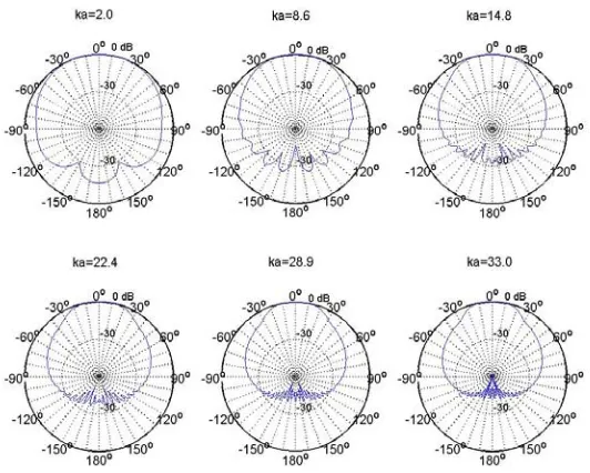
Figure 4 – y-z plane directivity for the source at 5m from an array of 128 microphones placed in the x-y plane

G

Guuiimmaarrããeess--PPoorrttuuggaall

paper ID: 132 /p.6

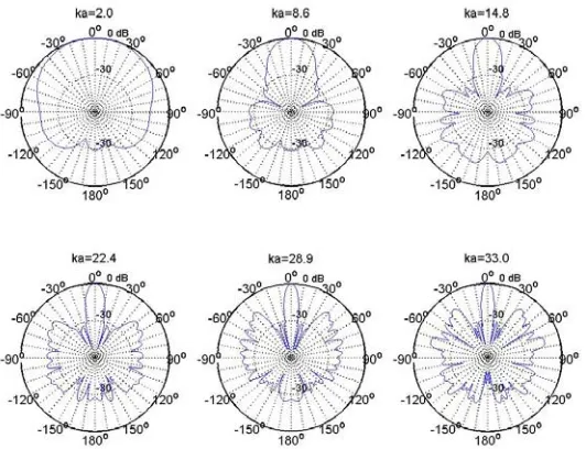
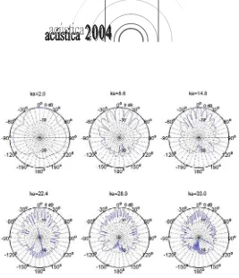
Figure 6 – y-z plane directivity for the source at 5m from an array of 128 microphones placed uniformly in a 9cm radius rigid sphere

The positioning of sensors in a random fashion helps to avoid the periodicity inherent in non-random arrangements, thus possibly flattening the co-array values [17].

G

Guuiimmaarrããeess--PPoorrttuuggaall

paper ID: 132 /p.7

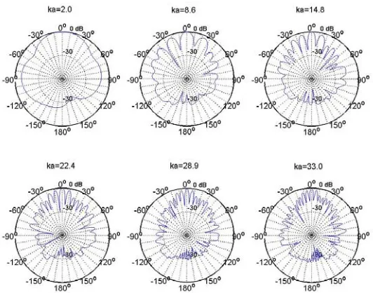
Figure 8 – y-z plane directivity for the source at5m from an array of 128 microphones placed randomly in a 9cm radius rigid sphere

4. CONCLUSIONS

Numerical experiments were undertaken, within a MATLAB environment, which compared the directivity performance of different microphone arrays. It was shown that when the microphones are placed uniformly around a sphere the directivity is better, since the mainlobe is narrower and there are less sidelobes than when the microphones are placed randomly or circularly around the sphere, the improvement goes up to 30dB.

REFERENCES

[1] M.J. Evans, A.I. Tew, J.A.S. Angus, Spatial Audio Teleconferencing - Which Way is

Better?, The Fourth International Conference on Auditory Display, Palo Alto, California

November, 1997.

[2] Y. Mahieux, G. Le Tourneur, A. Saliou, A Microphone Array for Multimedia

Workstations, Journal of the Audio Engineering Society 44 (5), May, 1996.

G

Guuiimmaarrããeess--PPoorrttuuggaall

paper ID: 132 /p.8

[4] J.L. Flanagan, D.A. Berkley, G.W. Elko, J.E. West, M.M. Sondhi., Autodirective

Microphone Systems, Acustica 73 (2): 58-71, February, 1991.

[5] B. Rafaely, Plane Wave Decomposition of the Sound Field on a Sphere by Spherical

Convolution, ISVR Technical Memorandum No. 910, University of Southampton, May, 2003.

[6] AES Staff Writer, Novel Surround Sound Microphone and Panning Techniques, A

digest of selected recent AES convention and conference papers, Journal of the Audio

Engineering Society 52 (1/2), January / February, 2004.

[7] B.N. Gover, J.G. Ryan, M.R. Stinson, Microphone Array Measurement System for

Analysis of Directional and Spatial Variations of Sound Fields, Journal of the Acoustical

Society of America 112 (5), Pt. 1, November, 2002.

[8] J.M. Rigelsford, A. Tennant, A 64 Element Acoustic Volumetric Array, Applied Acoustics 61: 469-475, 2000.

[9] J. Meyer, Beamforming for a Circular Microphone Array Mounted on Spherically

Shaped Objects, Journal of the Acoustical Society of America 109 (1): 185-193, January,

2001.

[10] J. Meyer, G.W. Elko, Echoes, The Newsletter of the Acoustical Society of America, Electroacoustic Systems for 3-D Audio – A report from the Pittsburgh meeting 12 (3), 2002.

[11] C. Cardoso, P. Nelson, Directivity of Spherical Microphone Arrays, In Proceedings of the Institute of Acoustics, Volume 26 (Part 2), Março, 2001.

[12] P.M. Morse, Vibration and Sound, McGraw-Hill Book Company, 1948.

[13] A. Tikhonov, V. Arsenin, Solution of Ill-Posed Problems, Winston, Washington D.C., 1977.

[14] P.A. Nelson, Source Strength Estimation in the Presence of Noise, unpublished notes, ISVR, University of Southampton, 2002.

[15] A.V. Oppenheim, R.W. Shaffer Digital Signal Processing, Prentice-Hall, London, 1975.

[16] C.A. Balanis, Antenna Theory: Analysis and Design, Wiley, New York, 1997.