O R I G I NA L A RT I C L E
Identification of asymmetric conditional
heteroscedasticity in the presence of outliers
M. Angeles Carnero1 · Ana Pérez2 · Esther Ruiz3
Received: 2 October 2014 / Accepted: 19 August 2015
© The Author(s) 2015. This article is published with open access at SpringerLink.com
Abstract The identification of asymmetric conditional heteroscedasticity is often based on sample cross-correlations between past and squared observations. In this paper we analyse the effects of outliers on these cross-correlations and, consequently, on the identification of asymmetric volatilities. We show that, as expected, one isolated big outlier biases the sample cross-correlations towards zero and hence could hide true leverage effect. Unlike, the presence of two or more big consecutive outliers could lead to detecting spurious asymmetries or asymmetries of the wrong sign. We also address the problem of robust estimation of the cross-correlations by extending some popular robust estimators of pairwise correlations and autocorrelations. Their finite sample resistance against outliers is compared through Monte Carlo experiments. Situations with isolated and patchy outliers of different sizes are examined. It is shown that a modified Ramsay-weighted estimator of the cross-correlations outperforms other esti-mators in identifying asymmetric conditionally heteroscedastic models. Finally, the results are illustrated with an empirical application.
Keywords Cross-correlations·Leverage effect·Robust correlations·EGARCH
JEL Classification C22
B
Esther Ruiz[email protected] M. Angeles Carnero [email protected] Ana Pérez
1 Department of Fundamentos del Análisis Económico, Universidad de Alicante, Alicante, Spain 2 Department of Economía Aplicada, Universidad de Valladolid, Valladolid, Spain
1 Introduction
One of the main topics that has focused the research of Agustín over a long period of time is seasonality. However, this is not his only topic of interest. Agustín’s con-tributions to the Econometric Time Series literature are much broader and include,
among others, the treatment of outliers in time series; see, for example,Maravall and
Peña(1986),Peña and Maravall(1991),Gómez et al.(1999) andKaiser and Maravall
(2003). In these papers, Agustín and his coauthors consider the effects and treatment
of outliers in macroeconomic data and, consequently, deal primarily with linear time series models. However, outliers are also present in the context of financial time series mainly when they are observed over long periods of time. It is important to note that, in this framework, the interest shifts from conditional means to conditional variances and, consequently, to non-linear models. Agustín has also contributions in this area; see Fiorentini and Maravall (1996) for an analysis of the dynamic dependence of second order moments.
When dealing with financial data, many series of returns are conditionally heteroscedastic with volatilities responding asymmetrically to negative and positive past returns. In particular, the volatility is higher in response to past negative shocks (‘bad’ news) than to positive shocks (‘good’ news) of the same magnitude. Following
Black(1976) this feature is commonly referred to asleverage effect. Incorporating the leverage effect into conditionally heteroscedastic models is important to better capture the dynamic behaviour of financial returns and improve the forecasts of future
volatility; seeBollerslev et al.(2006) for an extensive list of references andHibbert
et al.(2008) for a behavioral explanation of the negative asymmetric return–volatility relation. The identification of conditional heteroscedasticity is often based on the
sam-ple autocorrelations of squared returns.Carnero et al.(2007) show that the presence
of outliers biases these autocorrelations with misleading effects on the identification of time-varying volatilities. On the other hand, the identification of leverage effect is often based on the sample cross-correlations between past and squared returns. Nega-tive values of these cross-correlations indicate potential asymmetries in the volatility;
see, for example,Bollerslev et al.(2006),Zivot(2009),Rodríguez and Ruiz(2012) and
Tauchen et al.(2012). In this paper, we analyse how the identification of asymmetries, when based on the sample cross-correlations, can also be affected by the presence of outliers.
This paper has two main contributions. First, we derive the asymptotic biases caused
by large outliers on the sample cross-correlation of orderhbetween past and squared
observations generated by uncorrelated stationary processes. We show that klarge
consecutive outliers bias such correlations towards zero for h ≥ k, rendering the
detection of genuine leverage effect difficult. In particular, one isolated large outlier biases all the sample cross-correlations towards zero and so it could hide true leverage effect. Moreover, the presence of two big consecutive outliers biases the first-order
sample cross-correlation towards 0.5 (−0.5) if the first outlier is positive (negative)
and so it could lead to identify either spurious asymmetries or asymmetries of the wrong sign.
correlations and autocorrelations. In the context of bivariate Gaussian variables, there
are several proposals to robustify the pairwise sample correlation; seeShevlyakov
and Smirnov(2011) for a review of the most popular ones. However, the literature on robust estimation of correlations for time series is scarce and mainly focused on
autocovariances and autocorrelations. For example,Hallin and Puri(1994) propose
to estimate the autocovariances using rank-based methods. Ma and Genton(2000)
introduce a robust estimator of the autocovariances based on the robust scale
estima-tor ofRousseeuw and Croux(1992, 1993). More recently,Lévy-Leduc et al.(2011)
establish its asymptotic and finite sample properties for Gaussian processes.Ma and
Genton(2000) also suggest a possible robust estimator of the autocorrelation func-tion but they do not further discuss its properties neither apply it in their empirical
application. Finally,Teräsvirta and Zhao(2011) propose two robust estimators of the
autocorrelations of squares based on the Huber’s and Ramsay’s weighting schemes. The theoretical and empirical evidence from all these papers strongly suggests using robust estimators to measure the dependence structure of time series.
We analyse and compare the finite sample properties of the proposed robust esti-mators of the cross-correlations between past and squared observations of stationary uncorrelated series. As expected, these estimators are resistant against outliers remain-ing the same regardless of the size and the number of outliers. Moreover, even in the presence of consecutive large outliers, the robust estimators considered estimate the true sign of the cross-correlations although they underestimate their magnitudes. Among the robust cross-correlations considered, the modified version of the
Ramsay-weighted serial autocorrelation suggested byTeräsvirta and Zhao(2011) provides the
best resistance against outliers and the lowest bias.
To illustrate the results, we compute the sample cross-correlations and their robust counterparts of a real series of daily financial returns. We show how consecutive extreme observations bias the usual sample cross-correlations and could lead to wrongly identifying potential leverage effect. These empirical results enhance the importance of using robust measures of serial correlation to identify both conditional heteroscedasticity and leverage effect.
The rest of the paper is organized as follows. Section2is devoted to the
analy-sis of the effects of additive outliers on the sample cross-correlations between past and squared observations of stationary uncorrelated time series that could be either
homoscedastic or heteroscedastic. Section3considers four robust measures of
cross-correlation and compares their finite sample properties in the presence of outliers. The
difficulty of extending theMa and Genton(2000) proposal to the estimation of serial
cross-correlation is discussed in Sect.4. The empirical analysis of a time series of daily
Dow Jones Industrial Average index is carried out in Sect.5. Section6concludes the
paper with a summary of the main results and proposals for further research.
2 Effects of outliers on the identification of asymmetries
stationary processes that could be either homoscedastic or heteroscedastic. The main results are illustrated with some Monte Carlo experiments.
2.1 Asymptotic effects
Let yt,t = 1, ...,T, be a stationary series with finite fourth-order moment that is
contaminated from timeτ onwards bykconsecutive outliers with the same sign and
size,ω. The observed series is then given by
zt =
yt+ω if t =τ, τ+1, . . . , τ+k−1
yt otherwise. (1)
Denote byr12(h)the sample cross-correlation of orderh,h ≥1,between past and
squared observations ofzt, which is given by
r12(h)=
T t=h+1
zt−h−Z
(z2t −Z2)
T
t=1
zt−Z2Tt=1(z2t −Z2)2
(2)
whereZ = 1
T
T
t=1ztandZ2=
1
T
T
t=1z2t. The most pernicious impact of outliers
onr12(h)happens when they are huge and do not come up in the very extremes of the
sample but on such a position that they affect the two factors of the cross-products in
(2). In order to derive the impact of these outliers, we compute the limiting behaviour
ofr12(h)whenh+1≤τ ≤T −h−k+1 and|ω| → ∞.
The denominator of r12(h) in (2) can be written in terms of the original
uncontaminated seriesyt, as follows
t∈T0,0 yt2+
k−1
i=0
(yτ+i+ω)2−
1
T
⎡
⎣
t∈T0,0 yt+
k−1
i=0
(yτ+i +ω)
⎤ ⎦ 2 ×
t∈T0,0 y4t +
k−1
i=0
(yτ+i +ω)4−
1
T
⎡
⎣
t∈T0,0 yt2+
k−1
i=0
(yτ+i+ω)2
⎤ ⎦
2
(3)
whereTh,s= {t ∈ {h+1, ...,T}such thatt =τ+s, τ+s+1, . . . , τ +s+k−1}.
Since we are concerned with the limit as|ω| → ∞, we focus our attention on the terms
with the maximum power ofω. Then, it turns out that (3) is equal to
k−kT2
|ω|3+
o(ω3).
In order to make the calculations simpler, we consider the following alternative
expression of the numerator in (2), which is asymptotically equivalent if the sample
T
t=h+1
z2tzt−h−
1
T
T
t=h+1
zt2 T
t=h+1
zt−h
. (4)
Whenhis smaller than the number of consecutive outliers, i.e.h<k, expression (4)
can be written in terms of the original uncontaminated seriesyt, as follows
t∈Th,0∩Th,h
yt2yt−h+ h−1
i=0
(yτ+i+ω)2yτ+i−h+ k−1
i=h
(yτ+i +ω)2(yτ+i−h+ω)
+
k+h−1
i=k
yτ2+i(yτ+i−h+ω)
− 1
T
⎡
⎣
t∈Th,0 yt2+
k−1
i=0
(yτ+i +ω)2
⎤ ⎦
⎡
⎣
t∈Th,h yt−h+
k−1
i=0
(yτ+i+ω)
⎤
⎦. (5)
In expression (5), the terms with the maximum power ofωare the third and the fifth
ones, which containk−handk2terms inω3, respectively. Therefore, expression (5)
is equal to
k−h−kT2
ω3+o(ω3).
On the other hand, when the order of the cross-correlation is larger than the number
of outliers, i.e.h≥k, expression (4) can be written as follows
t∈Th,0∩Th,h
yt2yt−h+ k−1
i=0
(yτ+i +ω)2yτ+i−h+ k+h−1
i=h
yτ2+i(yτ+i−h+ω)+
−1
T
⎡
⎣
t∈Th,0 yt2+
k−1
i=0
(yτ+i+ω)2
⎤ ⎦
⎡
⎣
t∈Th,h yt−h+
k−1
i=0
(yτ+i+ω)
⎤
⎦. (6)
In this case, the term with the maximum power ofωis the fourth one, which contains
k2terms inω3. Therefore, expression (6) is equal to−kT2ω3+o(ω3).
Consequently, since the product in expression (3) is always positive, the sign of the
limit of the cross-correlations in (2) is given by the sign of its numerator, which in
turn depends on the sign ofω,and we get the following result:
lim
|ω|→∞r12(h)=
⎧ ⎨ ⎩
sign(ω)×
1− h
k(1−Tk)
ifh <k
sign(ω)×k−kT ifh ≥k.
(7)
Equation (7) shows that the effect of outliers on the sample cross-correlations depends
on: (1) whether the outliers are consecutive or isolated and (2) their sign. In particular,
one single large outlier (k=1 ) biasesr12(h)towards zero for all lags regardless of its
detection of genuine heteroscedasticity; seeCarnero et al.(2007). On the other hand,
a patch ofklarge consecutive outliers always biasesr12(h)towards zero for lagsh ≥
kand, for smaller lags, it generates positive or negative cross-correlations depending
on whether the outliers are positive or negative. For example, ifT is large, two huge
positive (negative) consecutive outliers generate a first order cross-correlation tending
to 0.5 (−0.5), being all the others close to zero; seeMaronna et al.(2006) andCarnero
et al.(2007) for a similar result in the context of sample autocorrelations of levels and squares, respectively. Therefore, if a heteroscedastic time series without leverage effect or an uncorrelated homoscedastic series is contaminated by several large negative consecutive outliers, the negative cross-correlations generated by the outliers can be
confused with asymmetric conditional heteroscedasticity.1In practice, we will not face
such huge outliers as to reach the limiting values ofr12(h)in (7), but the result is still
useful because it provides a clue on the direction of the bias of the cross-correlations. So far, we have assumed that the consecutive outliers have the same magnitude and sign. However, it could also be interesting to analyse the effects of outliers of different signs on the sample cross-correlations. For instance, one isolated positive (negative)
outlier in the price of an asset at timeτ, implies a doublet outlier in the corresponding
return series, i.e. a positive (negative) outlier at timeτfollowed by a negative (positive)
outlier at timeτ+1.In this case, we will havek=2 consecutive outliers of opposite
signs, that will be assumed, for the moment, to have equal magnitude, i.e. ωτ =
|ω|sign(ωτ)andωτ+1 = |ω|sign(ωτ+1). Then, ifh = 1 and the outlier size,|ω|,
goes to infinity, the largest contribution to the limit of the numerator ofr12(1)given
in (5) is due to the following term
(yτ+1+ωτ+1)2(yτ +ωτ)
and this is equal to |ω|3sign(ωτ). Therefore, the sign of the limit of the
cross-correlation is the sign of the first outlier: if this is positive and the second is negative,
the limit ofr12(1)as|ω| → ∞will be positive and equals to 0.5, while if the first
outlier is negative and the second is positive, the limit ofr12(1)as |ω| → ∞will
be negative and equals to−0.5. Forh ≥ 2,all the cross-correlationsr12(h)will go
to zero. A similar analysis can be carried out if the series is contaminated byk =3
consecutive outliers of the same size but different signs to know whether the limit of the cross-correlations is positive or negative.
Note also that the results above are still valid if the outliers have different sizes. In
this case, we can writeωt =ω+δt in (1) instead ofωand the results will be the same
when|ω| → ∞.
2.2 Finite sample effects
To further illustrate the results in the previous subsection, we generate 1000 artificial
series of sizeT =1000 by a homoscedastic Gaussian white noise process with unit
variance and by the EGARCH model proposed by Nelson (1991). The EGARCH
model generates asymmetric conditionally heteroscedastic time series and, according toRodríguez and Ruiz(2012), it is more flexible than other asymmetric GARCH-type models, to simultaneusly represent the dynamics of financial returns and satisfy the conditions for positive volatilities, covariance stationarity and finite kurtosis. The particular EGARCH model chosen to generate the data is given by
yt =σtεt
log(σt2)= −0.006+0.98 log(σt2−1)+0.2(|εt−1| −E(|εt−1|))−0.1εt−1
(8)
where εt is a Gaussian white noise process with unit variance and, consequently,
E(|εt−1|)=√2/π; seeNelson(1991) for the properties of EGARCH models. The
parameters in (8) have been chosen to imply a marginal variance of yt equal to one
and to resemble the values usually encountered in real empirical applications; see, for
instance,Hentschel(1995) andBollerslev and Mikkelsen(1999).2
Each simulated series is contaminated first, with a single negative outlier of size
ω= −50 at timet=500, and second, with two consecutive outliers of the same size
but opposite signs, the first negative (ω= −50) at timet=500 and the second positive
(ω=50) at timet=501. For each replicate, we compute the sample cross-correlations
up to order 50 and then, for each lag,h, we compute their average over all replicates.
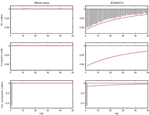
The first row of Fig.1plots the average sample cross-correlations from the
uncontam-inated white noise process (left panel) and for the uncontamuncontam-inated EGARCH process (right panel). The average sample cross-correlations computed from the correspond-ing contaminated series with one and two outliers are plotted in the second and third rows, respectively. In all cases, the red solid line represents the true cross-correlations. As we can see, when a series generated by the EGARCH model is contaminated with one single large negative outlier, we may wrongly conclude that there is not leverage effect since all the cross-correlations become nearly zero. On the other hand, when the series is contaminated with two consecutive outliers of different sign, being the first one negative, only the first cross-correlation will be different from zero and
approximately equal to −0.5 regardless of whether the series is homoscedastic or
heteroscedastic. Therefore, in this case, we can identify either a negative leverage effect when there is none (the series is truly a Gaussian white noise) or a much more negative leverage effect than the actual one (as in the case of the EGARCH model). Similar results would be obtained if the two outliers were positive, but in this case the
first cross-correlation would be biased towards 0.5.Consequently, we could wrongly
identify asymmetries in a series that is actually white noise or we could identify a positive leverage effect when it is truly negative as in the EGARCH process.
We now analyse how fast the limit in (7) is reached as the size of the outliers
increases. In order to do that, we contaminate the same 1000 artificial series simulated
before first with one isolated outlier of size{−ω}at timet =500 and second with two
consecutive outliers of sizes{−ω, ω}located at timest= {500,501}, whereωcould
2 We have also performed simulations with other EGARCH models with different parameter values and
0 10 20 30 40 50 -0,03
-0.06 0
White noise
sr
eil
t
u
o
o
N
0 10 20 30 40 50
-0,03 0
-0.06
EGAR C H
0 10 20 30 40 50
-0,03
-0.06 0
r
eil
t
u
o
e
vit
a
g
e
n
A
0 10 20 30 40 50
-0,03
-0.06 0
0 10 20 30 40 50
-0,4 -0,2 0
sr
eil
t
u
o
e
vit
u
c
e
s
n
o
c
o
w
T
Lag
0 10 20 30 40 50
-0,4 -0,2 0
Lag
Fig. 1 Monte Carlo means of sample cross-correlations in simulated white noise (first column) and EGARCH (second column) series without outliers (first row), with a single negative outlier (second row) and with two consecutive outliers, negative and positive (third row) of size|ω| =50. Thered solid linerepresents the true cross-correlations
take several values, namelyω = {1,2, ...,50}. We then compute the average of the
first and second order sample cross-correlations from these contaminated series over
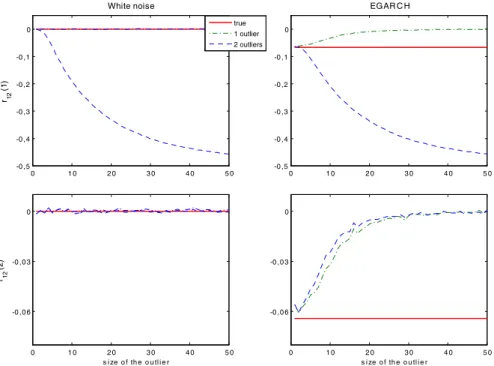
the 1000 replicates. Figure2plots the average ofr12(1)(first row) andr12(2)(second
row) against the size of the outlier,ω, for the two simulated processes and the two
types of contamination considered. The values of the theoretical cross-correlations for the uncontaminated processes are also displayed with a red solid line.
As we can see, the sample cross-correlations start being distorted when the outliers are larger (in absolute value) than 5 standard deviations. Furthermore, when the size of the outliers is over 20, the corresponding sample cross-correlations are already quite
close to their limiting values (−0.5 in the first order cross-correlation and 0 in the
0 1 0 2 0 3 0 4 0 5 0 -0 ,5
-0 ,4 -0 ,3 -0 ,2 -0 ,1 0
r21
)
1(
White noise
0 1 0 2 0 3 0 4 0 5 0
-0 ,5 -0 ,4 -0 ,3 -0 ,2 -0 ,1 0
EGAR C H
0 1 0 2 0 3 0 4 0 5 0
-0 ,0 6 -0 ,0 3 0
r21
)
2(
s i ze o f th e o u tl i e r
0 1 0 2 0 3 0 4 0 5 0
-0 ,0 6 -0 ,0 3 0
s i ze o f th e o u tl i e r true
1 outlier 2 outliers
Fig. 2 Monte Carlo means of sample cross-correlations of order 1 (first row) and of order 2 (second row) for white noise (first column) and EGARCH series (second column) contaminated with a single negative outlier and with two consecutive outliers, negative and positive, as a function of the outlier size. Thered solid linerepresents the true cross-correlation
3 Robust cross-correlations
In the previous section we have shown that the sample cross-correlations between past and squared observations of a stationary uncorrelated series are very sensitive to the presence of outliers and could lead to a wrong identification of asymmetries. In this section we consider robust cross-correlations to overcome this problem. In particular, we generalize some of the robust estimators for the pairwise correlations described inShevlyakov and Smirnov(2011) and one of the robust autocorrelations proposed byTeräsvirta and Zhao(2011). We discuss their finite sample properties and compare them to the properties of the sample cross-correlations.
3.1 Extensions of robust correlations
A direct way of robustifying the pairwise sample correlation coefficient between two random variables is to replace the averages by their corresponding nonlinear robust
counterparts, the medians; seeFalk(1998). By doing so in the sample cross-correlation
r12(h)in (2) we get the following expression, that is called thesample cross-correlation
median estimator:
r12,C O M E D(h)=
medt∈{h+1,...,T}{(zt−h−med(z))(z2t −med(z2))}
where med(x)stands for the sample median of x and M A D denotes the sample
median absolute deviation, i.e. M A D(x)= med(|x−med(x)|). Unless otherwise
stated, the median is calculated over the whole sample. When the median is calculated
over a subsample, this is specifically stated, as in (9), wheremedt∈{h+1,...,T}denotes
the sample median calculated over the subsample indexed byt ∈ {h+1, ...,T}.
Another popular robust estimator of the pairwise correlation is the Blomqvist quad-rant correlation coefficient. The extension of this coefficient to cross-correlations
yields the following expression, that will be called theBlomqvist cross-correlation
coefficient:
r12,B(h)=
1
T T
t=h+1
sign(zt−h−med(z))sign(z2t −med(z2)). (10)
Estimation of the correlation between two random variables XandY, denoted byρ,
can also be based on a scale approach, by means of the following identity:
ρ= V ar(U)−V ar(V)
V ar(U)+V ar(V) (11)
where
U =
X
σX + Y
σY
and V =
X
σX − Y
σY
(12)
are called the principal variables andσXandσY are the standard deviations ofX and
Y, respectively. In order to get robust estimators forρ,Gnanadesikan and
Ketten-ring(1972) propose replacing the variances and standard deviations in (11) and (12),
respectively, by robust estimators as follows
ρ= S2(U)−S2(V)
S2(U)+S2(V) (13)
where S is a robust scale estimator. Depending on the robust estimator S used in
(13), different robust estimators of the correlation may arise. For instance,Shevlyakov
(1997) considersSas the Hampel’s median of absolute deviations and gets the median
correlation coefficient. This estimator extended to compute cross-correlations, called
median cross-correlation coefficient, would be:
r12,M E D(h)=
medt∈{h+1,...,T}(|ut|)
2
−medt∈{h+1,...,T}(|vt|)
2
medt∈{h+1,...,T}(|ut|)
2
+medt∈{h+1,...,T}(|vt|)
2 (14)
where
ut = zt−h−med(z) M A D(z) +
z2t −med(z2)
M A D(z2) and vt =
zt−h−med(z) M A D(z) −
Finally, in the context of time series,Teräsvirta and Zhao(2011) propose robust esti-mators of the autocorrelations based on applying the Huber’s and Ramsay’s weights to the sample variances and autocovariances. We extend this idea to the cross-correlations
where the two series involved are the lagged levels, zt−h,and their squares, z2t. In
particular, we focus on the weighted correlation with the Ramsay’s weights using a slight modification to cope with squares. The resulting weighted estimator of the
cross-correlation of orderhproposed is given by
r12,W(h)= γ
12(h) √
γ1(0)γ2(0)
(15)
where
γ12(h)=
T
t=h+1wt−h
zt−h−Zw
w2
t(z2t −Zw2)
T
t=h+1wt−hw2t
,
γ1(0)=
T t=1wt
zt−Zw2
T t=1wt
and γ2(0)=
T t=1wt2
zt2−Z2
w
2
T t=1wt2
with
Zw =
T t=1wtzt
T t=1wt
, Z2
w =
T t=1wt2z2t
T t=1w2t
,
wt =exp
−a|zt−Z|
σz
and σz =
1
T −1
T t=1
zt −Z2.
FollowingTeräsvirta and Zhao(2011), we usea =0.3. By applying the weights
wt to the series in levels, every observation will be downweighted except those equal
to the sample mean. Note that when the weighting scheme is applied to squared observations, the weights are squared so that bigger squared observations are more downward weighted than their corresponding observations in levels.
3.2 Monte Carlo experiments
In order to analyse the finite sample properties of the four robust cross-correlations introduced above, we consider the same Monte Carlo simulations described in
Sect. 2.2. For each replicate, the robust cross-correlations are computed up to lag
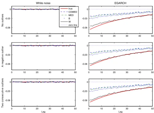
50. The first row of Fig. 3 plots the corresponding Monte Carlo averages for the
uncontaminated white noise process (left panel) and for the uncontaminated EGARCH
process (right panel). The second and third rows of Fig.3depict the averages of the
robust cross-correlations computed for the same series contaminated with one and two outliers, respectively. In all cases, the true cross-correlations are also displayed.
Several conclusions emerge from Fig. 3. First, as expected, robust measures of
note that the plots displayed in the first row are nearly the same to those displayed in the other two rows. Second, in EGARCH processes, the robust cross-correlations estimate the sign of the true cross-correlations properly but they underestimate their magnitude. In fact, the first three robust cross-correlations (r12,C O M E D,r12,Bandr12,M E D)
esti-mate asymmetries which are much weaker than the true ones. However, the weighted
cross–correlation,r12,W,performs quite well because its bias is much lower than those
of the other robust measures even in the presence of two big consecutive outliers.
Actu-ally, the values ofr12,W are very close to their theoretical counterparts. This could be
due to the fact that the first three robust measures considered are direct extensions of the corresponding robust estimators originally designed to estimate the pairwise correlation coefficient for a bivariate Gaussian distribution. In such framework, some of these measures, like the Blomqvist quadrant correlation and the median correlation coefficient are asymptotically minimax with respect to bias or variance. However, in time series data, and, in particular, in conditional heteroscedastic time series, none of these assumptions hold and hence the behaviour of these measures is not that good as postulated for the bivariate Gaussian case. Unlike, the Ramsay-weighted
autocorrela-tion estimator proposed byTeräsvirta and Zhao(2011) was already designed to cope
with time series data, and this could be the reason for the good performance ofr12,W
in estimating cross-correlations.
0 10 20 30 40 50
-0,06 -0.03 0 White noise sr eil t u o o N
0 10 20 30 40 50
-0.06 -0.03 0
EGARCH
0 10 20 30 40 50
-0.06 -0,03 0 r eil t u o e vit a g e n A
0 10 20 30 40 50
-0.06 -0,03 0
0 10 20 30 40 50
-0.06 -0,03 0 sr eil t u o e vit u c e s n o c o w T Lag
0 10 20 30 40 50
-0.06 -0,03 0 Lag true COMED MED B W zero line
Fig. 3 Monte Carlo means of robust cross-correlations in simulated white noise (first column) and EGARCH (second column) series without outliers (first row), with a single negative outlier (second row) and with two consecutive outliers, negative and positive (third row) of size|ω| =50. Thered solid line
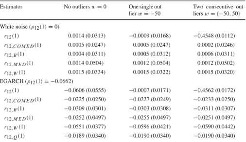
Table 1 Monte Carlo means and standard deviations of several estimators of the first-order cross-correlation between past and current squared observations from uncorrelated stationary processes
Estimator No outliersw=0 One single out-lierw= −50
Two consecutive out-liersw= {−50,50} White noise (ρ12(1)=0)
r12(1) 0.0014 (0.0313) −0.0009 (0.0168) −0.4548 (0.0112)
r12,C O M E D(1) 0.0005 (0.0247) 0.0005 (0.0247) 0.0002 (0.0246) r12,B(1) 0.0004 (0.0311) 0.0005 (0.0312) 0.0006 (0.0311)
r12,M E D(1) 0.0014 0.0504) 0.0012 (0.0504) 0.0012 (0.0502) r12,W(1) 0.0015 (0.0334) 0.0015 (0.0322) 0.0015 (0.0320)
EGARCH (ρ12(1)= −0.0662)
r12(1) −0.0606 (0.0555) −0.0007 (0.0171) −0.4562 (0.0172)
r12,C O M E D(1) −0.0225 (0.0250) −0.0227 (0.0249) −0.0233 (0.0250) r12,B(1) −0.0309 (0.0301) −0.0303 (0.0308) −0.0311 (0.0307)
r12,M E D(1) −0.0252 (0.0497) −0.0255 (0.0497) −0.0251 (0.0497)
r12,W(1) −0.0551 (0.0377) −0.0596 (0.0421) −0.0590 (0.0442) r12,Q(1) −0.0189 (0.0340) −0.0190 (0.0340) −0.0190 (0.0340) Sample size is T = 1000 and the number of replications is 1000
We also perform a similar analysis to that in Sect. 2.2, by studying the effect
of the size of the outliers on the four robust cross-correlations for the two types of
contamination, namely contamination with one isolated outlier of size{−ω}and with
two consecutive outliers of sizes{−ω, ω}, whereω= {1,2, ...,50}.The results, which
are not displayed here to save space but are available upon request, are as expected. Robust cross-correlations remain the same regardless of the size and the number of outliers. Moreover, they all subestimate the magnitude of the leverage effect, but
the bias in the weighted cross-correlation,r12,W, is negligible as compared to the
alternative robust cross-correlations considered.
So far, we have analysed the Monte Carlo mean cross-correlograms for different lags and sizes of the outliers. In order to complete these results, we next study the whole
finite sample distribution of the cross-correlations considered focusing on the first lag.3
Table1reports the Monte Carlo means and standard deviations (in parenthesis) of the
first order sample cross-correlation, as defined in (2), and of the four robust
cross-correlations introduced in Sect.3.1, for the two processes, Gaussian white noise and
EGARCH, and for the two types of contamination; Fig.4displays the corresponding
box-plots.
As expected, when the series is a homoscedastic Gaussian white noise and there are no outliers or there is one isolated outlier, all estimators behave similarly and the sample cross-correlations perform very well. Note that, in this case, the sample correlation is the maximum likelihood estimator of its theoretical counterpart and therefore it is consistent and asymptotically unbiased and efficient. Unlike, the robust
SA M P L E CO M E D ME D Q W -0 .2 -0 .1 0 0. 1 0. 2 W h it e no is e
s r e i l t u o o N
SA M P L E CO M E D ME D Q W -0 .2 0 0. 2 EG A R C H SA M P L E CO M E D ME D Q W -0 .2 -0 .1 0 0. 1 0. 2
r e i l t u o e v i t a g e n g i b A
SA M P L E CO M E D ME D Q W -0 .2 -0 .1 0 0. 1 0. 2 SA M P L E CO M E D ME D Q W -0 .4 -0 .2 0
s r e i l t u o e v i t u c e s n o c o w T
estimators have, in general, slightly larger dispersion since they are not as efficient as maximum likelihood estimators. However, when there are two consecutive outliers, the sample cross-correlation breaks down and it becomes unreliable: its distribution is completely pushed downwards and it would be estimating a large negative asymmetry when there is none. Unlike, all the robust estimators considered perform very well in
terms of bias andr12,C O M E D(1)also performs quite well in terms of variance.
When the simulated process is an EGARCH, another picture comes up. When the
series is not contaminated, either the sample cross-correlation,r12(1), or the weighted
cross–correlation,r12,W(1), performs better than any of the other robust measures
originally designed to estimate pairwise correlations in bivariate Normal distributions. However, when the EGARCH series is contaminated by one single negative outlier, the sample cross-correlation is pushed upwards towards zero, as postulated from the
theoretical results in Sect.2, and it would be unable to detect the true leverage effect
in the data. The situation becomes even worse in the presence of two consecutive outliers, where the sample cross-correlation becomes completely unreliable due to its huge negative bias. As expected, the distribution of all the robust cross-correlations remain nearly the same regardless of the presence of outliers. However, the estimators
r12,C O M E D(1),r12,B(1)andr12,M E D(1), in spite of their robustness, are upwards
biased towards zero and so they will underestimate the true leverage effect. Unlike,
the weighted sample cross-correlation with the modified Ramsay’s weights,r12,W(1),
performs surprisingly well in terms of bias, even in the presence of two big outliers.
As it happened with the simulated white noise process, the estimatorr12,M E D(1)has
the largest standard deviation of all the estimators considered; see Table1. Therefore,
it seems that the robust cross-correlationr12,W(1)is preferable to any other
mea-sure considered in this section for the identification of asymmetries in conditionally heteroscedastic models.
4 Discussion
In the previous section, we analyse the finite sample performance of several robust
estimators of the cross-correlations, including the estimator in (13) withSdefined as
the Hampel’s median of absolute deviations. Other possible choices forSare the robust
scale estimatorsSn andQn proposed byRousseeuw and Croux(1993).Shevlyakov
and Smirnov(2011) show that the robust estimator of the pairwise correlation between
bivariate Gaussian variables based onQnperforms better than other robust correlation
estimators. Ma and Genton (2000) suggest bringing this approach to estimate the
autocorrelation of Gaussian time series. In this section, we show that this extension is not so straight when the processes involved are non-Gaussian.
Let us consider replacing the scale estimatorS in Eq. (13) by the highly efficient
robust scale estimator Qnproposed byRousseeuw and Croux (1992, 1993). Given
the sample observationsx=(X1, ...,Xn)from a distribution function FX, the scale
estimatorQnis based on an order statistic of alln2pairwise distances and it is defined
as follows:
Qn(x)=c(FX)Xi−Xj,i < j
where{X}(k)denotes thek-th order statistic of X,k≈
n
2
/4 for largen andc(FX)
is a constant, that depends on the shape of the distribution function FX,introduced
to achieve Fisher consistency. In particular, ifFXbelongs to the location-scale family
Fμ,σ(x)=F((x−μ)/σ), the constant is chosen as follows
c(F)=1/(K−F1(5/8)),
whereKFis the distribution function ofX−X, beingXandXindependent random
variables with distribution functionF; seeRousseeuw and Croux(1993). In particular,
in the Gaussian case(F =), the constant is:
c()=1/(√2−1(5/8))=2.21914.
Althoughc(FX)can also be computed for various other distributions, the FORTRAN
code provided byCroux and Rousseeuw(1992) and the MATLAB Library for Robust
Analysis (https://wis.kuleuven.be/stat/robust/LIBRA) developed at
ROBUST@Leu-ven, compute the estimatorQnwith the Gaussian constantc().4
In the time series setting,Ma and Genton (2000) propose the following robust
estimator of the serial autocorrelation. Let y=(Y1, ...,YT)be the observations of
a stationary process Yt and let ρ(h) = Corr(Yt−h,Yt) be the corresponding
autocorrelation function. In this case, the variables X andY in (12) represent two
variables,Yt−handYt, with the same model distribution and, consequently,σX =σY.
Therefore, using identity (12) withσX =σY, plugging the scale estimatorQnin (13)
and taking into account thatQnis affine equivariant, i.e.Qn(a X+b)= |a|Qn(X),
the robust estimator ofρ(h)would be:
ρQ(h)=
Q2T−h(u)−Q2T−h(v)
Q2T−h(u)+Q2T−h(v) (17)
where uis a vector of lengthT −h defined asu = (Y1+Yh+1, , ...,YT−h+YT)
andvis another vector of lengthT −hdefined asv=(Y1−Yh+1, , ...,YT−h−YT).
Ma and Genton(2000) argue that the estimatorρQ(h)is independent of the choice of
the constants needed to compute the scale estimatorsQninvolved in (17). In another
framework,Fried and Gather(2005) use the estimatorρQ(1)and also state that such
constants cancel out. However, as we show bellow, the constants do not cancel out in general and this simplification only applies for Gaussian variables. By rewriting
Qn(x)=c(FX)Q∗n(x)where Q∗n(x)=Xi −Xj,i< j
(k), the estimator ρQ(h)
in (17) becomes:
ρQ(h)=
c2(FU)Q∗T2−h(u)−c2(FV)Q∗T2−h(v)
c2(FU)Q∗2
T−h(u)+c2(FV)Q∗T2−h(v)
(18)
4 Note that the algorithm inCroux and Rousseeuw(1992) also includes a correction factor to improve
where FU and FV denote the cumulative distribution functions of Yt−h +Yt and
Yt−h−Yt, respectively. Note that this estimator requires computingc(FU)andc(FV).
AsLévy-Leduc et al.(2011) point out, this is easily done in the Gaussian case, where
c(FU)=c(FV)=2.21914; otherwise, the problem could become unfeasible.
More-over, the constants only cancel out if c(FU) = c(FV), but this condition is rarely
achieved, unless the processYt is Gaussian.
Turning back to the estimation of cross-correlations between past and squared observations of uncorrelated stationary processes, the situation becomes even more
tricky. In this case, the two series involved are the lagged levels, Yt−h, and its
own squares,Yt2, which are not equally distributed neither Gaussian. Furthermore,
the variables X and Y in (12) will stand for Yt−h and Yt2 and so the constraint
σX = σY no longer holds. Hence, the first step to compute the robust
estima-tor of ρ12(h) = Corr(Yt−h,Yt2), based on identities (11) and (12), will be to
‘standardize’ the two series involved. LetYt = Yt/QT(y)andY2
t = Yt2/QT(y2)
denote the robust ‘standardized’ forms of the seriesYt andY2
t , respectively, where
QT(y) = c(FY)Q∗T(y)and QT(y2) = c(FY2)Q∗T(y2). The second step will be to
form the vector of sums and the vector of differences:
u=(Y1+Yh2+1, , ...,YT−h+YT2),
v=(Y1−Yh2+1, , ...,YT−h−Y 2
T).
The third step will be to calculate the robust variance estimates of these two vectors,
Q2T−h(u)andQ2T−h(v), respectively, and finally, replace these variance estimators in
(11) and obtain the following estimator ofρ12(h):
r12,Q(h)=
c2(FU)QT∗2−h(u)−c2(FV)QT∗2−h(v)
c2(F
U)Q∗T2−h(u)−c2(FV)Q∗T2−h(v)
(19)
where FU and FV denote the cumulative distribution functions of Yt−h +Yt2 and
Yt−h−Yt2, respectively.
Therefore, it is clear that the estimator (19) will require computing four constants,
c(FY),c(FY2),c(FU)andc(FV), but this task seems to be unfeasible. Note that, even
ifYwere Gaussian,Y2would be no longer Gaussian, neitherY+Y2norY−Y2would
be. Moreover, even if we could compute the constants in such case, the assumption of
Gaussianity forY would be unsuitable, because the distribution of financial returns is
known to be heavy-tailed.
To further illustrate what would it happen if we ignored the constants and proceed as in the Gaussian setting, we repeat the same Monte Carlo experiment described in previous sections for the EGARCH model, computing for each replicate the estimator
r12,Q(1)in (19) with all constants equal toc(). The Monte Carlo means and
stan-dard deviations are reported in the last row of Table1. As expected, the results are
disappointing: the estimatorr12,Q turns out to be the most biased among the robust
estimators considered and it also has larger variance than both r12,C O M E D(1)and
Hence, one should be very cautious before implementing robust estimators origi-nally designed for bivariate Gaussian distributions in a time series setting with potential non-Gaussian variables.
5 Empirical application
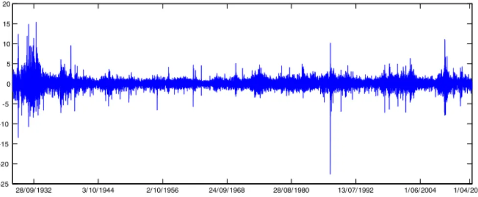
In this section we illustrate the previous results by analyzing a series of daily Dow Jones Industrial Average (DJIA) returns observed from October 2, 1928 to August
30, 2013, comprising 21409 observations. This is the series considered byCharles
and Darné(2014). Figure5plots the data. As expected, the returns exhibit the usual volatility clustering, along with some occasional extreme values that could be regarded as outliers, the largest one corresponding to October 19, 1987, when the index collapsed by −22.6 %. Charles and Darné(2014) apply the procedure proposed by Laurent et al. (2014) to detect and correct additive outliers in this return series and show that large shocks in the volatility of the DJIA are mainly due to particular events (financial crashes, US elections, wars, monetary policies, etc.), but they also find that some shocks are not identified as outliers due to their occurring during high volatility periods.
In order to show how the potential outliers can mislead the detection of the leverage effect, as measured by the cross-correlations between past and squared returns, we use a rolling window scheme, where the sample size used to compute the cross-correlations
isT =1000.Therefore, we first estimate the cross-correlations over the period from 2
October 1928 to 28 September 1932. When a new observation is added to the sample, we delete the first observation and re-estimate the cross-correlations. This process is repeated until we reach the last 1000 observations in the sample, from November 2,
2009 to August 30, 2013. This amounts to considering 20,410 different subsamples
covering periods of different volatility levels and different types and sizes of outliers. For instance, the first subsample, runing from 2 October 1928 to 28 September 1932,
28/ 09/ 1932 3/ 10/ 1944 2/ 10/ 1956 24/ 09/ 1968 28/ 08/ 1980 13/ 07/ 1992 1/ 06/ 2004 1/ 04/ 2013 -25
-20 -15 -10 -5 0 5 10 15 20
28/09/1932 3/10/1944 2/10/1956 24/09/1968 28/08/1980 13/07/1992 1/06/2004 1/04/2013 -0.3
-0.2 -0.1 0 0.1
28/09/1932 3/10/1944 2/10/1956 24/09/1968 28/08/1980 13/07/1992 1/06/2004 1/04/2013 -0.3
-0.2 -0.1 0 0.1
sample robust confidence bands
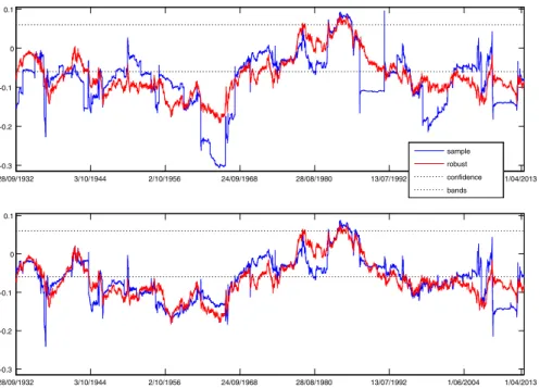
Fig. 6 Sample and robust first order cross-correlations computed with subsamples of size T=1000 using a rolling window of both the DJIA daily returns (top panel) and its outlier-corrected counterpart (bottom panel). The dates in thex-axisrefer to the end-of-window dates
includes outliers associated with the 1929 Stock market crash, while the 13900t h
subsample, corresponding to observations from 21 March 1984 to 4 March 1988, includes outliers due to the 1987 Stock market crash. For each subsample considered,
we compute the first order sample cross-correlation, r12(1),using Eq. (2) and the
corresponding robust weighted cross-correlation,r12,W(1),as defined in Eq. (15), for
both the original return series and the outlier-adjusted return series of Charles and
Darné(2014)5. Figure6displays the values of these cross-correlations for the 20410 subsamples considered. Note that the dates in the x-axis refer to the end-of-window
dates. Figure 6 also displays the 95 % confidence bands based on the asymptotic
distribution of the sample cross-correlations under the null of zero cross-correlations; seeFuller(1996). These bands are only shown for guidance, since not all the conditions for the asymptotic results to hold are fulfilled in our setting. Nevertheless, it is worth noting that the standard deviation predicted by the asymptotic theory for samples
of size T = 1000 is aproximately 0.032, which is just the value of the standard
deviation ofr12,W(1)in our Monte Carlo experiments with a white noise process; see
Table1.
Several conclusions emerge from Fig. 6. First, this figure clearly reveals how
extreme observations can bias the sample cross-correlation and could lead to a wrong identification of asymmetries. As expected, the 1st order sample cross-correlation,
r12(1), presents several sharp drops and rises when it is computed for the original
returns (top panel) and it is quite different from its robust counterpart. These changes are generally associated with the entrance and/or exit of outlying observations in the corresponding subsample. For instance, the entrance of the “Black Monday” October
19, 1987, where the DJIA sustained its largest 1-day drop (y14804= −22.61),
follow-ing another large negative return (y14804= −4.60), conveys a sudden fall in the value
ofr12(1)from nearly zero to a negative value around−0.17. Unlike, the next sudden
rise in the value ofr12(1),from nearly−0.11 to a positive value around 0.10, is due to
the consecutive exit from the corresponding subsamples of the “Black Monday” and
two adjacent extreme observations,y14805 =5.88 (19/10/1987) and y14806 =10.15
(21/10/1987). When these three observations, the first one being negative and the
other two positive, are in the subsample, the value ofr12(1)is pushed downwards
to a negative value, but when the first of these observations leaves the sample and
only the positive outliers remain,r12(1)is pushed upwards to a value even larger than
zero, as postulated by our theoretical result in Sect.2. Moreover, the bunch of lowest
negative values ofr12(1), ranging from−0.25 to−0.3, is related to the entrance/exit
in the corresponding subsamples of two consecutive extreme observations, namely
y8422 = −5.71 (28/5/1962) and y8423 =4.68 (29/5/1962), the former being
identi-fied as an outlier inCharles and Darné(2014). According to our theoretical result in
Sect.2, the entrance of these two observations, the first one being negative and the
second positive, biases downwards the first-order sample cross-correlation, but when the first of these observations leaves the sample and only the positive outlier remains,
r12(1)is again pushed to a value closer to zero. Similarly, the following sharp rise
inr12(1)from around−0.17 to−0.05 is due to an isolated positive outlier, namely
y8799=4.50 (26/11/1963).
Another remarkable feature from Fig.6is the difference between the values of the
sample cross-correlation in the top and bottom panels, enhancing the little resistance of
r12(1)to the presence of outliers. Unlike, the weighted cross-correlation,r12,W(1), is
robust to the presence of potential outliers: its values remain nearly the same in the two panels, indicating that the leverage effect suggested by the sample cross-correlation could be misleading in some cases.
Noticeable, the weighted robust and the sample 1st order cross-correlations are quite similar when computed for the outlier-corrected series (bottom panel), but the latter still exhibits some breaks even in this case. These breaks are associated with
extreme observations that were not identified as outliers neither corrected inCharles
and Darné(2014). For instance, the first sharp drop inr12(1)from around−0.10 to
−0.24 and its immediate rise again to−0.10, have to do with the presence/absence of
two couples of outliers: a doublet positive outlier made up ofy1130=9.03 (19/4/1933)
andy1131=5.80 (20/4/1933) and a doublet negative outlier made up ofy1194= −7.07
(20/7/1933) and y1195 = −7.84 (21/7/1933). A similar situation arises at one of the
last subsamples, where the value ofr12(1)decays towards−0.22; such a big drop is
associated with the entrance of three consecutive extreme observations at the end of
the subsample, namelyy20162 = −5.07 (19/11/2008),y20163 = −5.56 (20/11/2008)
andy20164=6.54 (21/11/2008), which, according to our theoretical result in Sect.2,
Finally, Fig.6highlights that the value of the robust cross-correlation,r12,W(1),
does not remain constant across all the subsamples considered. This feature suggests
time-varying leverage effects, with periods wherer12,W(1)is nearly zero (possibly
indicating no leverage) followed by periods where r12,W(1)clearly takes negative
values (leverage effect). In particular, there seems to be three sample periods where
the leverage effect, as measured byr12,W(1), seems to be stronger: a first period at the
beginning of the sample, from April 1933 till June 1936, a second long period that spans from July 1940 till April 1971, aproximately, and a final period from around September 1989 till the end of the sample. Notice that only along these periods the robust sample cross-correlations are outside the approximated 95 % asymptotic confidence bands. Obviously, this feature requires further investigation; see, for instance, the recent
papers ofBandi and Renò(2012),Yu(2012) andJensen and Maheu(2014) dealing
with time-varying leverage effects.
6 Conclusions
This paper shows that outliers can severely affect the identification of the asymmetric response of volatility to shocks of different signs when this is performed based on the sample cross-correlations between past and squared returns. In particular, the presence of one isolated outlier biases such cross-correlations towards zero and hence could hide true leverage effect while the presence of two big outliers could lead to detect either spurious asymmetries or asymmetries of the wrong sign. As a way to protect against the pernicious effects of outliers, we suggest using robust cross-correlations. Our Monte Carlo experiments show that, among the robust measures considered in this paper, the weighted cross-correlation based on a slight modification of the serial
correlation with Ramsay’s weights proposed byTeräsvirta and Zhao(2011), seems
to be the more appropriate when dealing with conditionally heteroscedastic models. These results are further illustrated in the empirical application. It is shown that the first order sample cross-correlation between past and squared daily DJIA returns is harmfully affected by the presence of outliers, while its robust counterpart is not. In fact, depending on which measure of cross-correlation is used, the detection of asymmetries could be misleading. It is also shown that some observations which are not identified as outliers may still have a distorting effect on the identification of asymmetries in the volatility, enhancing the advantages of using robust methods as a protection against outliers rather than detecting and correcting them. The empirical application also prompts to the existence of possible time-varying leverage effects. We leave this topic for further research along with the problem of robust estimation of asymmetric GARCH models.
Open Access This article is distributed under the terms of the Creative Commons Attribution 4.0 Interna-tional License (http://creativecommons.org/licenses/by/4.0/), which permits unrestricted use, distribution, and reproduction in any medium, provided you give appropriate credit to the original author(s) and the source, provide a link to the Creative Commons license, and indicate if changes were made.
References
Bandi F, Renò R (2012) Time-varying leverage effects. J Econom 169:94–113
Black R (1976) Studies in stock price volatility changes. In: Proceedings of the 1976 business meeting of the business and economics statistics sections, American Statistical Association, pp 177–181 Bollerslev T, Litvinova J, Tauchen G (2006) Leverage and volatility feedback effects in high-frequency
data. J Financ Econom 4:353–384
Bollerslev T, Mikkelsen HO (1999) Long-term equity anticipation securities and stock market volatility dynamics. J Econom 92(1):75–99
Carnero MA, Peña D, Ruiz E (2007) Effects of outliers on the identification and estimation of GARCH models. J Time Ser Anal 28(4):471–497
Charles A, Darné O (2014) Large shocks in the volatility of the Dow Jones Industrial Average index: 1928–2013. J Bank Financ 43:188–199
Croux C, Rousseeuw PJ (1992) Time-effcient algorithms for two highly robust estimators of scale. In: Dodge Y, Whittaker J (eds) Comput Stat, vol 1. Physika-Verlag, Heidelberg, pp 411–428
Falk M (1998) A note on the comedian for elliptical distributions. J Multivar Anal 67(2):306–317 Fiorentini G, Maravall A (1996) Unobserved components in ARCH models: an application of seasonal
adjustment. J Forecast 15(3):175–201
Fried R, Gather U (2005) Robust trend estimators for AR(1) disturbances. Austrian J Stat 34(2):139–151 Fuller WA (1996) Introduction to statistical time series, 2nd edn. Wiley, Hoboken
Gnanadesikan R, Kettenring JR (1972) Robust estimates, residuals and outlier selection with multiresponse data. Biometrics 28:81–124
Gómez V, Maravall A, Peña D (1999) Missing observations in ARIMA models: skipping approach versus additive approach. J Econom 88:341–363
Hallin M, Puri ML (1994) Aligned rank tests for linear models with autocorrelated error term. J Multivar Anal 50:175–237
Hentschel L (1995) All in the family: nesting symmetric and asymmetric GARCH models. J Financ Econo 39:71–104
Hibbert AM, Daigler RT, Dupoyet B (2008) A behavioral explanation for the negative asymmetric return-volatility relation. J Bank Financ 32:2254–2266
Jensen MJ, Maheu JM (2014) Estimating a semiparametric stochastic volatility model with a Dirichlet process mixture. J Econom 178:523–538
Kaiser R, Maravall A (2003) Seasonal outliers in time series. Estadística (J Interam Stat Inst) 15:101–142 Laurent S, Lecourt C, Palm FC (2014) Testing for jumps in Gaussian ARMA-GARCH models, a robust
approach. Comput Stat Data Anal. doi:10.1016/j.csda.2014.05.015
Lévy-Leduc C, Boistard H, Moulines E, Taqqu MS, Reisen VA (2011) Robust estimation of the scale and of the autocovariance function of Gaussian short- and long-range dependent processes. J Time Ser Anal 32:135–156
Ma Y, Genton MG (2000) Highly robust estimation of the autocovariance function. J Time Ser Anal 21:663– 684
Maravall A, Peña D (1986) Missing observations and additive outliers in time series models. In: Mariano RS (ed) Advances in statistical analysis and statistical computing. JAI Press, Stanford
Maronna R, Martin D, Yohai V (2006) Robust Statistics: theory and methods. Wiley, Hoboken
Nelson DB (1991) Conditional heteroskedasticity in asset returns: a new approach. Econometrica 59(2):347– 370
Peña D, Maravall A (1991) Interpolation, outliers and inverse autocorrelations. Commun Stat Theory Methods 20(10):3175–3186
Rodríguez MJ, Ruiz E (2012) GARCH models with leverage effect: differences and similarities. J Financ Econom 10:637–668
Rousseeuw PJ, Croux C (1993) Alternatives to the median absolute deviation. J Am Stat Assoc 88:1273– 1283
Shevlyakov G (1997) On robust estimation of a correlation coefficient. J Math Sci 83(3):434–438 Shevlyakov G, Smirnov P (2011) Robust estimation of the correlation coefficient: an attempt of survey.
Austrian J Stat 40(1):147–156
Tauchen G, Bollerslev T, Sizova N (2012) Volatility in equilibrium: asymmetries and dynamic dependencies. Rev Financ 16:31–80
Teräsvirta T, Zhao Z (2011) Stylized facts of return series, robust estimates and three popular models of volatility. Appl Financ Econ 21:67–94
Yu J (2012) A semiparametric stochastic volatility model. J Econom 167:473–482 Zakoian JM (1994) Threshold heteroskedastic models. J Econ Dyn Control 18:931–955