C
C
|
E
E
|
D
D
|
L
L
|
A
A
|
S
S
Centro de Estudios
Distributivos, Laborales y Sociales
Maestría en Economía Universidad Nacional de La Plata
Assessing Benefit-Incidence Results Using
Decompositions: The Case of Health Policy in
Argentina
Leonardo Gasparini
Assessing Benefit-Incidence Results using Decompositions
The case of Health Policy in Argentina 1
Leonardo Gasparini
CEDLAS
Universidad Nacional de La Plata*
Abstract
This paper discusses the use of aggregate and microeconometric decompositions to compare benefit-incidence results over time and across regions. Decompositions are applied to explore changes in targeting in health policies directed to pregnant women and children under 4 in Argentina. The results suggest that although health public programs are pro-poor, incidence changes in the last 5 years have been pro-rich due to two different factors: a substantial reduction in the fertility rate of poor couples, and an increase in the use of public facilities by wealthier households, likely triggered by the economic crisis that Argentina has suffered since 1998.
Keywords: health, children, targeting, decompositions, Argentina
JEL classification: D3, I1, I38. 1
This paper is the follow-up of a study on targeting health and nutrition policies in Argentina written by the author in FIEL for the World Bank’s Thematic Group on Health, Nutrition and Population and Poverty. I am grateful to the outstanding research assistance of Julieta Trías (UNLP) and Eugenia Orlicki (FIEL). I am also grateful to seminar participants at the World Bank and Universidad Nacional de La Plata, and Davidson Gwatkin, Mónica Panadeiros, Daniel Bergna and two anonymous referees in the World Bank for useful comments and suggestions.
*
Centro de Estudios Distributivos, Laborales y Sociales (CEDLAS) de la Universidad Nacional de La Plata. Calle 6 entre 47 y 48, oficina 516, 1900 La Plata, Argentina. Tel-fax: 54-221-4229383.
1. Introduction
A benefit-incidence analysis allows an assessment of the degree of targeting of average public spending. Although incidence results of particular programs are useful on their own, more can be learnt from the comparison of results over time and across regions. This paper illustrates the usefulness of decomposition techniques to shed light on the factors behind differences in benefit-incidence results between time periods, regions or programs.
In particular, changes in the benefit-incidence results for a particular health service are decomposed into three components: (i) changes in individual and household characteristics linked to the decision to consume that health service, (ii) changes in the way decisions whether to consume the service or not are made, and (iii) changes in the public/private decision to where to consume the service. Both aggregate and microeconometric decompositions are implemented to provide estimates of these three components. Results of the decompositions are useful for the understanding of the reasons why a given health program has become less or more pro-poor over time, or why a program is less or more pro-poor in one region than in another.
two different factors: a substantial reduction in the fertility rate of poor couples, and an increase in the use of public facilities by wealthier households, likely triggered by the economic crisis that Argentina has suffered since 1998.
The rest of the study is organized as follows. Section 2 shows the results from a typical benefit-incidence analysis for different health services. Section 3 is the core of the paper as aggregate and microeconometric decomposition techniques are introduced, and the main results are shown and discussed. Some brief comments in section 4 close the paper.
2. Benefit-incidence results
Argentina has had a disappointing economic performance over the last three decades. Figure 2.1 shows large cyclical fluctuations in the disposable mean income, without signs of an increasing trend. The vertical lines in the Figure indicate the period covered by this analysis, 1997 to 2001, a period of substantial income fall. Per capita disposable income in real terms fell 13% between 1997 and 2001 according to National Accounts estimates. Along with a stagnant economy, Argentina has suffered dramatic transformations in its income distribution.2 Inequality and poverty have substantially increased over the last three decades, and in particular in the period 1997-2001.
Benefit-incidence analysis is aimed at evaluating the degree of targeting of average public spending in a specific program. Benefits from the program are assigned to individuals according to their answers to a household survey on the program use.3 We first describe the data used for the analysis and then present and discuss the basic results.
The data
Benefit-incidence analyses require household surveys with data on a welfare indicator and information on the use of social programs. In the last decade Argentina has conducted two Living Standard Surveys with questions on the use of various health and nutrition services. The first survey, known as Encuesta de Desarrolo Social (EDS), was conducted in 1996/7 and includes 73,410 individuals (representing 83% of total
2
See Gasparini (2003). 3
population) living in urban areas. The second survey, Encuesta de Condiciones de Vida (ECV), with similar coverage and questionnaires, was conducted in 2001.
Both surveys include questions on housing, some assets, demographics, labor variables, health status and services, and education. The EDS and ECV were sponsored by The World Bank and have questionnaires similar to those in other countries.4 However, they are not part of the Living Standard Measurement Surveys (LSMS) program and they do not include questions on expenditures as the LSMS surveys do.5
Welfare indicators
A crucial stage in a benefit-incidence analysis is sorting households by a welfare indicator. Among the variables usually included in a household survey household consumption adjusted for demographics is the best proxy for individual welfare (Deaton and Zaidi, 2002). Unfortunately, most household surveys in Argentina, including the EDS and the ECV, do not have household-expenditures questions. This paper uses household income adjusted for demographics, or equivalized household income, as the individual welfare indicator. Equivalized household income y for each individual is defined as
Heckman (2002). For benefit-incidence analysis in Argentina see Flood et al. (1993), Harriague and Gasparini (1999), Gasparini et al. (2000) and DGSC (2002).
4
See http://www.siempro.gov.ar/Encuesta%20de%20desarrollo%20social/encuesta%202001/encuesta.htm
for more information on the surveys. 5
(
α α)
θ2 2 1
1K K
A
Y y
+ +
=
where Y is total household income, A is the number of adults in the household, K1 the
number of children under 5, and K2 the number of children aged 6 to 14. Parameters αs
allow for different weights for adults and kids, while θ regulates the degree of household
economies of scale. Following Deaton and Zaidi (2002) and given the characteristics of the Argentinean economy, we take intermediate values of the αs (α1=0.5 and α2=0.75),
and a rather high value of θ (0.9) as the benchmark case. Per capita household income
can also be viewed as a particular case of equivalized income with no differential weights (all αs equal to 1) and no economies of scale (θ=1).
In Table 2.1 individuals with consistent answers and positive reported household income are grouped in quintiles. The table shows mean income of each quintile for the distribution of per capita household income and equivalized household income. Argentina underwent a recession between 1998 and 2002, which shows up in Table 2.1: incomes fell along the distribution.
The use of health services and nutrition programs
the number of children per household is decreasing in income, the share of children is not uniform along the income distribution. For instance, the share of children under 4 was 30.1 in the bottom quintile and 12.1 in the top quintile in 1997. This fact will have a fundamental consequence on the distributional incidence of public programs directed to children. Even a universal program to all children will be pro-poor, given the negative correlation between the number of children and household income. This relationship became less strong between 1997 and 2001, as a consequence of a fall in the fertility of low-income families relative to the rest,6 implying, other things equal, a potential reduction in the targeting of social policies.
The public sector finances public health facilities. These resources allow public hospitals and centers to provide health services free of charge or at subsidized prices. Who are the beneficiaries of this subsidy? A usual assumption is that the users of the service and their families are the beneficiaries of the public program. By using a public health service free of charge a family saves the cost of buying that service, which is assumed to be equal to the average cost of public provision.7
Table 2.3 shows benefit-incidence results for five health services: antenatal care, attended deliveries, visits to doctors, free medicines and hospitalizations. More details on each of these services and results for other services can be obtained from a companion paper (Gasparini and Panadeiros, 2004). Subsidies to antenatal care in public facilities are
6
highly pro-poor. In 1997 more than 46% of total beneficiaries of this program belonged to the first quintile of the income distribution. The share of beneficiaries from the top quintile was 2%. The degree of targeting of the public subsidy to antenatal care decreased between 1997 and 2001. Similar results are obtained for the rest of the health services.
Table 2.4 shows the concentration index (CI) of each service, a measure of the extent to which a particular variable is distributed unequally across the income strata (see Lambert, 1993). Negative numbers reflect pro-poor programs. The higher the CI in absolute value the more pro-poor the program.
Concentration indices are computed from household survey data. Surveys are just a sample of the population. Even with a stable population the computed value of an index may change if we take two different samples. Hence, it is important to compute the statistical significance of the changes in a given statistic, like the CI. This practice is a rigorous way of assessing whether the recorded change in the statistic is large enough to be reasonably confident on the fact that the statistic also changed in the population. Although benefit-incidence results are typically subject to the problem of sample variability, they are never complemented with a statistic-significance analysis. In this paper confidence intervals are computed using bootstrapping techniques.8 Table 2.4 shows the limits of the 95% confidence interval below the value of each CI estimate.
7
All health programs considered are pro-poor. The free delivery of medicines seems to be the most pro-poor program. Between 1997 and 2001 there has been a decrease in the degree of targeting in all health services. This fall is illustrated in Figure 2.2 where all the concentration curves for the health programs in 2001 are below the corresponding curves for 1997. The next section explores these changes with the help of decompositions.
3. Characterizing changes in targeting
Benefit-incidence results come from aggregating individual decisions on the consumption of publicly provided services. A household will consume a given service if (i) at least one of its members is eligible for that service, (ii) she (or her parents) decides to consume the service, and (iii) she decides to do it in the public sector. Accordingly, differences in targeting of a given program over time or across regions are the result of differences in the three stages described above. It is relevant to identify to what extent the change in the degree of targeting for a given program is the result of changes in the socio-demographic structure of the population, or the result of changes in the household decisions on the consumption of the service (whether to consume the service or not, and where to do it). In this section this question is tackled using aggregate and microeconometric decompositions.
8
Aggregate decompositions
Suppose we group total population in quintiles h=1,…,5 according to their equivalized household income. The proportion of total users of a given health service j in a public facility that belong to quintile h in time t is denoted as bhjt. These proportions are the
inputs of any benefit-incidence measure. If bhjt is decreasing in income, it is said that the
public program j is “pro-poor”. The value bhjtcan be written as
hjt hjt hjt
hjt q a p
b = . .
where qhjt is the proportion of people who qualify for service j who belong to quintile h,
ahjt is the rate of use of service j in quintile h relative to the population mean, while phjt is
the share of users in the public sector in h relative to the population mean. Differences among quintiles in the value of b are driven by differences in q, a, and p.
The relative use of a given service (summarized by a) is the second determinant of the incidence results. Keeping all the other things constant, if in contrast to pregnant women from rich households, most women from poor households decide not to see a medically-trained person for antenatal care, the value of a will be increasing in income. Finally, the choice public/private is the third crucial determinant of the incidence results. If poor pregnant women choose a public facility more often than rich women, the value of p will be decreasing in income.
Differences in the pattern of the bs, and then in the incidence results over time and across regions depend on differences in the right-hand-side factors of the previous equations. We use this simple decomposition to get a preliminary characterization of differences in incidence results over time and across regions in Argentina.
Table 3.1 shows the results of the decomposition of incidence results by quintiles for different health programs. The first three panels in each table reproduce results for q, a, and
p. The distribution of potential users, the participation decision and the choice public/private determine the incidence results of the fourth panel. The differences in incidence by quintile are reported in row 5.
the top quintile. Where does this reduction in targeting come from? The last panel helps us to characterize the incidence changes by showing decomposition results. The line labeled
potential users shows incidence results if we change the distribution of pregnant women (first panel) between 1997 and 2001 but we keep fixed the participation rates and the public/private decisions at the values of a given year. Since the values of a and p can be fixed at two alternative years, in the Table we report the average over the 4 possible simulations.
The distribution of pregnant women became less pro-poor between 1997 and 2001, implying a 1.4 drop in the incidence on the bottom quintile. This means that everything constant, the demographic changes would explain a sizeable part of the decrease in the degree of targeting of the subsidy to antenatal care in public hospitals and primary health centers. Poor women are now more likely to be seen by medically trained persons. This increase in participation (combined with the changes for the rest of the distribution) implies an increase in incidence on the bottom quintile of 0.9 points. The last effect, labeled public provision, seems the most relevant one: although the use of public hospitals increased for poor people it increased proportionally more for the rest of the population. This effect implies a sizeable drop in the degree of targeting in the bottom quintile.
public facilities by non-poor women. In contrast with the case of antenatal care, the first effect seems to be the dominant one. Similar results are obtained for the case of public subsidies to medicines. The incidence of public hospital admissions increased a bit for the bottom quintile, and decreased a lot for the second one, leading to a fall in the overall degree of targeting as measured by the concentration index. This fall for the second quintile is explained by a relative reduction in fertility, a large drop in the share of hospitalized children, and a less pronounced increased in the use of public facilities, compared to other quintiles of the distribution.
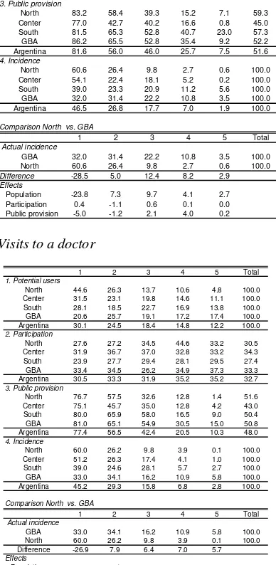
Aggregate decompositions can also be applied to study differences in incidence results across regions. Table 3.2 shows results for deliveries and visits to doctors in 1997.9 Differences between two regions in incidence results are the consequence of differences in the distribution of potential users, the participation rates and the choice of public facilities. The Table shows the decomposition of differences between the North and GBA. Similar results can be obtained for any other two regions from the information of the Table. There is a substantial difference in the degree of targeting of the public subsidy to deliveries in public hospitals between the North and GBA. Most of that difference comes from a much more concentrated distribution of children under 4 in the bottom quintile of the national
income distribution in the North than in GBA. While 19.5% of children under 4 in GBA belong to the bottom quintile of the national distribution of equivalized household income, that share rises to 44.1% in the North. 23.8 out of the 28.5 points of the incidence
9
difference for the bottom quintile between the two regions are explained by this population effect. If all women chose public hospitals to have their babies, a subsidy to deliveries in public facilities would be more pro-poor in the North, since the population in that region is considerable poorer than in the GBA. In the North even without much effort for a better targeting, public programs are usually more pro-poor.
In addition to the population effect, the difference in targeting in favor of the North is accounted by a less intensive use of public facilities by the rich in the North compared to the GBA. Similar results apply to visits to doctors in 1997 and to all health services in 2001 (see Table 3.3).
Microeconometric decompositions (microsimulations)
characteristics of each individual (and her family), (ii) the way these characteristics are linked to the decision of visiting a doctor, and (iii) the way these characteristics are linked to the choice of attending a public facility instead of a private one.
To implement this methodology we estimate econometric models of the decision of visiting a doctor, and the conditional decision of attending a public facility as functions of various individual and household characteristics. Changes in the concentration index are decomposed into three effects. The population effect is obtained by simulating the health decisions in time t if the individual and household characteristics were those of time t´; the participation effect comes from simulating each individual’s health decisions in time t
if the parameters that govern the decision to visit a doctor were those of time t´, while the
public provision effect is computed by assuming that the parameters governing the public/private decision were those of time t´.
To explain the methodology analytically, suppose there are there are N individuals indexed with i=1, …,N. Each individual i is defined by a vector of individual observable characteristics Xi and a vector of individual unobservable characteristics Ui. Individual
characteristics include age, gender, education as well as household characteristics as income and location.
People who qualify for a given health service j can use a private or a public provider. Let
bijt be a binary variable that identifies people who get the service j in the public sector at
10
time t (beneficiaries of public expenditures in the program j). As before, this variable can be expressed as
ijt ijt ijt
ijt q a p
b = . .
where now q is equal to 1 if the individual qualifies for the service and 0 otherwise, a is equal to 1 if the individual decides to use the health service and 0 otherwise, and p is 1 if the individual uses a public provider. Variable q is deterministic:
) , ( it jt
ijt Q X
q = α
Given observable characteristics Xi an individual qualifies or not for the service (e.g.
being pregnant qualifies for antenatal care). The vector of parameters α determines the
rule of access to a given service.
Variables a and p instead are random variables as they depend on unobservable factors.
) , ,
( it it jt
ijt A X U
a = β
) , , ( it it jt
ijt P X U
p = γ
) , , , ,
( it it jt jt jt
ijt B X U
b = α β γ
A measure of distributional incidence of public expenditures in service j is a combination of the distribution of b and of certain characteristics Y of the vector X (e.g. household income)
}) { }, ({ ijt it
jt I b Y
I =
where Y ∈X. Hence,
) , , }, { },
({ it it jt jt jt
jt F X U
I = α β γ
A similar equation can be derived for other time period t1
) , , }, { },
({ 1 1 1 1 1
1 it it jt jt jt
jt F X U
I = α β γ
We define three effects in which the change in I between t and t1 can be decomposed:
Participation effect ) , , }, { }, ({ ) , , }, { },
({ it1 it1 jt1 jt1 jt1 it1 it1 jt1 jt jt1
j F X U F X U
This effect captures the change in incidence resulting from a change in the parameters governing the decision of consuming a given service (β).
Public-provision effect ) , , }, { }, ({ ) , , }, { },
({ it1 it1 jt1 jt jt1 it1 it1 jt1 jt jt
j F X U F X U
PP = α β γ − α β γ
This effect measures the change in incidence as the consequence of changes in the parameters governing the public/private decision.
Population effect ) , , }, { }, ({ ) , , }, { },
({ it1 it1 jt jt jt it it jt jt jt
j F X U F X U
PO = α β γ − α β γ
This effect measures changes in incidence resulting from changes in the distribution of observable and unobservable characteristics of the population.
Assuming α does not change, the change in I can be expressed as
j j j
j PA PP PO
I = + +
∆
Some of the functions and parameters in the decomposition are either know or assumed, and some should be estimated. We observe the function and parameters that determine
potential users (Q and α) and vector X. We assume a form for A and P, and propose a
benefit-incidence index I. We estimate parameters β and γ and the vector of
unobservables U.
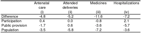
Table 3.4 reports the results of performing the decompositions. The first row shows the change in the absolute value of the concentration index between 1997 and 2001 for each health service, while the last three rows show the values of each of the effects. The concentration index for the program of antenatal care in public facilities went down 4.8 points between 1997 and 2002, implying lower targeting. If only the way individual decisions on pregnancy controls are taken had changed between 1997 and 2001, the CI would have increased 0.4 points, which represents a negligible change. The effect of the changing public/private decisions between 1997 and 2001 contributed with 1.7 points in the overall fall of the CI. The most significant factor in this fall was the change in the population characteristics. Even with all parameters kept constant, the change in characteristics would have contributed to the reduction in the CI with 3.5 points. The reduction in the number of children in poor families is likely the main factor behind this result.
attended deliveries, likely reflecting an increasing number of middle and high-income groups attending public hospitals as the result of the economic crisis. The participation effect is negligible in all cases, except for hospitalizations, which is a sign of the increase in hospitalizations for children from the poorest quintile.
4. Concluding remarks
References
Bourguignon, F., Lustig, N. and Ferreira, F. (eds.) (2003). The Microeconomics of Income Distribution Dynamics, forthcoming.
Bourguignon, F., Pereira da Silva, L. and Stern, N. (2002). Evaluating the poverty impact of economic policies: some analytical challenges. Mimeo, The World Bank.
Carneiro, P., Hansen, K., and Heckman, J. (2002). Removing the veil of ignorance in assessing the distributional impacts of social policies. Mimeo, University of Chicago.
CEDLAS (2003). Estadísticas distributivas en la Argentina. Centro de Estudios
Distributivos, Laborales y Sociales, Departamento de Economía, Universidad Nacional de La Plata.
Deaton, A. and Zaidi, S. (2002). Guidelines for constructing consumption aggregates for welfare analysis. LSMS Working Paper 135.
DGSC (2002). El impacto distributivo de la política social en la Argentina. Dirección de Gastos Sociales Consolidados. Secretaría de Política Económica, Ministerio de Economía.
social: Argentina, 1991. Anales de la XXVIII Reunión de la Asociación Argentina de Economía Política, Tucumán.
Gasparini, L. (director) (2000). El impacto distributivo del gasto público en sectores sociales en la Provincia de Buenos Aires. Un análisis en base a la Encuesta de Desarrollo Social. Cuadernos de Economía 50, La Plata.
Gasparini, L. (2003). Argentina´s distributional failure. Mimeo, IADB.
Gasparini, L. and Panadeiros, M. (2004). Targeting health and nutrition policies. The case of Argentina. World Bank’s Thematic Group on Health, Nutrition and Population and Poverty
Harriague, M. and Gasparini, L. (1999). El impacto redistributivo del gasto público en los sectores sociales. Anales de la XXXIV Reunión de la Asociación Argentina de Economía Política, Rosario.
Lambert, P. (1993). The distribution and redistribution of income. Manchester University Press.
Marchionni, M. and Gasparini, L. (2003). Tracing out the effects of demographic changes on the income distribution. The case of Greater Buenos Aires, 1980-2000.
Mills, J. and Zandvakili, S. (1997). Statistical inference via bootstrapping for measures of inequality. Journal of Applied Econometrics 12, 133-150.
Sosa Escudero, W. and Gasparini, L. (2000). A note on the statistical significance of changes in inequality. Económica XLVI (1). Enero-Junio.
van de Walle, D. and Nead, K. (1995). Public Spending and The Poor: Theory and Evidence. Johns Hopkins University Press for the World Bank.
Table 2.1
Mean incomes by quintile
Distribution of equivalized household income
Per capita income Equivalized income
1997 2001 1997 2001
(i) (ii) (iii) (iv)
1 54.6 38.1 75.4 52.7
2 120.9 93.0 159.6 121.9
3 196.9 156.9 248.8 198.4
4 321.1 263.9 393.6 322.1
5 853.9 704.6 1000.1 823.9
Mean 309.5 251.3 375.6 303.8
[image:25.612.90.271.261.332.2]Source: authors´ calculations based on the EDS and ECV.
Table 2.2
Children by quintiles
Distribution of equivalized household income
Children under Children under 2 years-old 4 years-old
1997 2001 1997 2001
(i) (ii) (i) (ii)
1 29.7 27.6 30.1 27.8
2 24.6 21.7 24.5 21.6
3 19.1 20.1 18.4 20.4
4 13.6 15.6 14.8 15.6
5 13.0 15.1 12.1 14.6
Total 100.0 100.0 100.0 100.0
[image:25.612.89.275.391.536.2]Source: authors´ calculations based on the EDS and ECV.
Table 2.3
Benefit-incidence results
Distribution of equivalized household income
1 2 3 4 5 Tota
1. Antenatal care
1997 46.5 26.8 17.7 7.0 2.0 100.0
2001 43.3 26.8 19.3 8.0 2.5 100.0
Change -3.2 0.0 1.6 1.0 0.6 0.0
2. Attended deliveries
1997 44.5 27.7 17.9 7.1 2.7 100.0
2001 41.9 27.0 18.4 9.5 3.2 100.0
Change -2.6 -0.8 0.5 2.4 0.4 0.0
3. Visits to a doctor
1997 45.1 29.6 15.6 6.9 2.8 100.0
2001 43.2 27.5 19.1 6.7 3.4 100.0
Change -1.9 -2.1 3.6 -0.1 0.6 0.0
4. Medicines
1997 51.6 26.1 14.8 6.1 1.4 100.0
2001 49.4 21.7 16.3 8.7 3.9 100.0
Change -2.2 -4.4 1.4 2.6 2.5 0.0
5. Hospitalizations
1997 42.5 35.0 15.1 5.9 1.5 100.0
2001 44.5 17.5 27.1 9.1 1.8 100.0
Change 2.0 -17.5 12.0 3.2 0.3 0.0
l
[image:25.612.93.246.596.675.2]Source: authors´ calculations based on the EDS and ECV.
Table 2.4
Concentration indices
Health services 1997 2001 Antenatal care -46.9 -42.9
(-48.4, -45.8) (-44.5,-41.1)
Attended delivery -45.3 -41.4
(-46.4, -43.8) (-43.0,-39.1)
Visits to a doctor -44.0
(-44.9, -43.1)
Medicines -51.0 -38.7
(-53.5, -48.4) (-41.7,-36.6)
Hospitalizations -46.6 -37.2
(-49.9, -44.3) (-43.3,-33.1)
Source: authors´ calculations based on the EDS and ECV.
Table 3.1
Aggregate decomposition of incidence results Health services, 1997 and 2001
Antenatal care
1 2 3 4 5 Total
1. Potential users
1997 29.7 24.6 19.1 13.6 13.0 100.0 2001 27.6 21.7 20.1 15.6 15.1 100.0
2. Participation
1997 94.8 96.3 99.5 99.4 98.4 97.1 2001 97.6 96.5 97.6 98.5 99.2 97.7
3. Public provision
1997 81.6 56.0 46.0 25.7 7.6 51.6 2001 85.6 68.1 52.4 27.7 9.0 54.9
4. Incidence
1997 46.5 26.8 17.7 7.0 2.0 100.0 2001 43.3 26.8 19.3 8.0 2.5 100.0
5. Difference -3.2 0.0 1.6 1.0 0.6
6. Effects
Potential users -1.4 -2.1 1.7 1.4 0.4 Participation 0.9 -0.2 -0.5 -0.1 0.0 Public provision -2.7 2.4 0.4 -0.2 0.1
Attended deliveries
1 2 3 4 5 Tota
1. Potential users
1997 29.7 24.6 19.1 13.6 13.0 100.0
2001 27.6 21.7 20.1 15.6 15.1 100.0
2. Participation
1997 98.3 99.4 99.9 100.0 100.0 99.3
2001 98.3 99.4 99.9 100.0 100.0 99.3
3. Public provision
1997 79.5 59.4 49.1 27.3 10.9 53.4
2001 83.4 67.5 49.5 33.0 11.3 55.0
4. Incidence
1997 44.5 27.7 17.9 7.1 2.7 100.0
2001 41.9 27.0 18.4 9.5 3.2 100.0
5. Difference -2.6 -0.8 0.5 2.4 0.4
6. Effects
Potential users -1.5 -2.2 1.7 1.5 0.6
Participation 0.0 0.0 0.0 0.0 0.0
Public provision -1.1 1.5 -1.2 1.0 -0.1
l
Medicines
1 2 3 4 5 Tota 1. Potential users
1997 30.1 24.5 18.4 14.8 12.1 100.0 2001 27.8 21.6 20.4 15.6 14.6 100.0 2. Participation
1997 24.2 25.6 26.6 28.5 26.2 25.9 2001 51.6 52.0 57.8 54.8 63.1 55.5 3. Public provision
1997 49.7 29.2 21.4 10.1 3.1 27.2 2001 64.8 36.4 25.9 19.1 8.0 32.3 4. Incidence
1997 51.6 26.1 14.8 6.1 1.4 100.0 2001 49.4 21.7 16.3 8.7 3.9 100.0 5. Difference -2.2 -4.4 1.4 2.6 2.5 6. Effects
Potential users -1.7 -1.9 2.3 0.7 0.6 Participation 0.6 -0.9 0.6 -0.6 0.3 Public provision -1.1 -1.6 -1.5 2.6 1.6
l
Hospitalizations
1 2 3 4 5 Tota 1. Potential users
1997 30.1 24.5 18.4 14.8 12.1 100.0 2001 27.8 21.6 20.4 15.6 14.6 100.0 2. Participation
1997 8.8 10.6 6.9 7.1 7.0 8.4 2001 9.6 6.8 10.9 9.1 4.5 8.4 3. Public provision
1997 84.3 70.5 62.1 29.1 9.2 63.1 2001 91.9 66.0 67.3 35.1 15.0 65.4 4. Incidence
1997 42.5 35.0 15.1 5.9 1.5 100.0 2001 44.5 17.5 27.1 9.1 1.8 100.0 5. Difference 2.0 -17.5 12.0 3.2 0.3 6. Effects
Potential users -1.8 -2.2 3.0 0.6 0.4 Participation 2.7 -12.2 8.7 1.6 -0.8 Public provision 1.1 -3.2 0.4 0.9 0.7
l
Table 3.2
Aggregate regional decomposition of incidence results, 1997
Deliveries
1 2 3 4 5 Tota
1. Potential users
North 44.1 26.4 14.6 10.0 4.8 100.0 Center 32.1 23.2 19.7 13.7 11.3 100.0 South 27.5 20.3 22.7 15.6 13.9 100.0 GBA 19.5 25.4 20.6 15.2 19.3 100.0 Argentina 29.7 24.6 19.1 13.6 13.0 100.0
2. Participation
North 94.5 98.0 98.0 99.7 97.9 96.6 Center 95.7 99.2 100.0 99.5 99.9 98.3 South 98.2 99.0 98.3 100.0 99.6 98.9 GBA 93.4 92.6 100.0 99.0 97.6 96.1 Argentina 94.8 96.3 99.5 99.4 98.4 97.1
3. Public provision
North 83.2 58.4 39.3 15.2 7.1 59.3 Center 77.0 42.7 40.2 16.6 0.8 45.0 South 81.5 65.3 52.8 40.7 23.0 57.3 GBA 86.2 65.5 52.8 35.4 9.2 52.2 Argentina 81.6 56.0 46.0 25.7 7.5 51.6
4. Incidence
North 60.6 26.4 9.8 2.7 0.6 100.0 Center 54.1 22.4 18.1 5.2 0.2 100.0 South 39.0 23.3 20.9 11.2 5.6 100.0 GBA 32.0 31.4 22.2 10.8 3.5 100.0 Argentina 46.5 26.8 17.7 7.0 1.9 100.0
Comparison North vs. GBA
1 2 3 4 5 Tota
Actual incidence
GBA 32.0 31.4 22.2 10.8 3.5 100.0 North 60.6 26.4 9.8 2.7 0.6 100.0
Difference -28.5 5.0 12.4 8.2 2.9
Effects
Population -23.8 7.3 9.7 4.1 2.7 Participation 0.4 -1.1 0.6 0.1 0.0 Public provision -5.0 -1.2 2.1 4.0 0.2
l
l
Visits to a doctor
1 2 3 4 5 Tota
1. Potential users
North 44.6 26.3 13.7 10.6 4.8 100.0
Center 31.5 23.1 19.8 14.6 11.1 100.0
South 28.1 18.5 22.7 16.9 13.8 100.0
GBA 20.6 25.7 19.1 17.2 17.4 100.0
Argentina 30.1 24.5 18.4 14.8 12.2 100.0
2. Participation
North 27.6 27.2 34.5 44.6 33.2 30.5
Center 31.9 36.7 37.0 32.8 33.2 34.3
South 23.9 27.7 29.4 28.1 29.5 27.4
GBA 33.4 34.5 26.2 34.9 37.3 33.3
Argentina 30.5 33.3 31.9 35.2 35.2 32.7
3. Public provision
North 76.7 57.5 32.6 12.8 1.4 51.6
Center 75.1 45.7 35.0 12.8 4.2 43.0
South 80.0 65.9 58.0 16.5 9.0 50.4
GBA 81.0 65.1 54.9 30.5 15.0 50.8
Argentina 77.4 56.5 42.4 20.5 10.3 48.0
4. Incidence
North 60.0 26.2 9.8 3.9 0.1 100.0
Center 51.2 26.3 17.4 4.1 1.0 100.0
South 39.0 24.6 28.1 5.7 2.7 100.0
GBA 33.0 34.1 16.2 10.9 5.8 100.0
Argentina 45.2 29.3 15.8 6.8 2.8 100.0
Comparison North vs. GBA
1 2 3 4 5 Tota
Actual incidence
GBA 33.0 34.1 16.2 10.9 5.8 100.0
North 60.0 26.2 9.8 3.9 0.1 100.0
Difference -26.9 7.9 6.4 7.0 5.7
Effects
Population -22.8 7.4 7.7 5.2 2.5
Participation 3.5 3.9 -5.0 -2.5 0.1
Public provision -7.5 -3.5 3.6 4.4 3.0
l
l
Table 3.3
Aggregate regional decomposition of incidence results Comparison North vs. GBA
Health services, 2001
Antenatal care
1 2 3 4 5 Tota
1. Actual incidence
GBA 31.8 26.0 27.0 10.8 4.4 100.0 North 60.9 25.4 8.9 4.3 0.5 100.0
2. Difference -29.1 0.6 18.0 6.5 4.0
3. Effects
Population -19.5 -0.9 11.3 6.6 2.5 Participation 1.1 -1.4 -0.4 0.5 0.1 Public provision -10.8 2.9 7.1 -0.6 1.3
Deliveries
1 2 3 4 5 Tota
1. Actual incidence
GBA 42.0 21.2 25.5 8.0 3.2 100.0 North 63.8 25.4 7.0 3.4 0.3 100.0
2. Difference -21.8 -4.2 18.5 4.6 2.9
3. Effects
Population -19.2 1.0 10.9 5.4 1.8 Participation 0.3 -0.9 0.6 0.1 0.0 Public provision -3.0 -4.3 7.0 -0.8 1.0
Visits to doctors
1 2 3 4 5 Tota
1. Actual incidence
GBA 33.5 30.0 20.4 10.4 5.7 100.0 North 57.8 25.8 10.7 4.5 1.2 100.0
2. Difference -24.4 4.2 9.8 5.9 4.5
3. Effects
Population -22.7 1.8 9.8 6.8 4.3 Participation 0.8 3.9 -3.7 -1.1 0.2 Public provision -2.4 -1.4 3.8 0.2 -0.1
Medicines
1 2 3 4 5 Tota
1. Actual incidence
GBA 37.0 13.8 18.5 22.9 7.9 100.0 North 64.2 25.0 5.2 4.7 0.9 100.0
2. Difference -27.2 -11.2 13.3 18.2 7.0
3. Effects
Population -24.8 2.0 6.9 11.3 4.6 Participation -8.1 5.0 2.0 0.0 1.2 Public provision 6.0 -18.4 4.3 7.0 1.0
Hospitalizations
1 2 3 4 5 Tota
1. Actual incidence
GBA 38.2 8.5 40.8 12.4 0.0 100.0 North 65.9 21.6 6.5 5.4 0.6 100.0
2. Difference -27.7 -13.1 34.3 7.1 -0.6
3. Effects
Population -24.9 1.8 13.0 9.4 0.7 Participation -1.8 -5.7 5.5 2.5 -0.6 Public provision -1.0 -9.4 15.8 -4.3 -1.1
l
l
l
l
l
Table 3.4
Microeconometric decompositions (Microsimulations)
Change in the absolute value of the concentration index 1997-2001
Antenatal Attended Medicines Hospitalizations care deliveries
(i) (ii) (iii) (iv) Difference -4.8 -5.2 -11.6 -7.2 Participation 0.4 0.0 -0.8 2.1 Public provision -1.7 0.6 -3.6 -5.7 Population -3.5 -5.8 -7.2 -3.6
Figure 2.1
Mean disposable income Argentina, 1980-2002 1980=100 70 75 80 85 90 95 100 105 110 115 120
1980 1981 1982 1984 1985 1986 1987 1988 1989 1990 1991 1992 1993 1994 1995 1996 1997 1998 1999 2000 2001 2002
Source: CEDLAS (2003).
Figure 2.2
Concentration curves
Antenatal care, attended delive ry, medicines and hospitalizations, 1997 and 2001
Pregnancy control Attended delivery
Medicines Hospitalizations 0 0.1 0.2 0.3 0.4 0.5 0.6 0.7 0.8 0.9 1
0 0.1 0.2 0.3 0.4 0.5 0.6 0.7 0.8 0.9 1 1997 2001 Lorenz
0 0.1 0.2 0.3 0.4 0.5 0.6 0.7 0.8 0.9 1
0 0.1 0.2 0.3 0.4 0.5 0.6 0.7 0.8 0.9 1 1997 2001 Lorenz
0 0.1 0.2 0.3 0.4 0.5 0.6 0.7 0.8 0.9 1
0 0.1 0.2 0.3 0.4 0.5 0.6 0.7 0.8 0.9 1 1997 2001 Lorenz
0 0.1 0.2 0.3 0.4 0.5 0.6 0.7 0.8 0.9 1
[image:30.612.89.483.311.569.2]SERIE DOCUMENTOS DE TRABAJO DEL CEDLAS
Todos los Documentos de Trabajo del CEDLAS están disponibles en formato electrónico en <www.depeco.econo.unlp.edu.ar/cedlas>.
• Nro. 18 (Febrero, 2005). Leonardo Gasparini. "Assessing Benefit-Incidence Results Using Decompositions: The Case of Health Policy in Argentina".
• Nro. 17 (Enero, 2005). Leonardo Gasparini. "Protección Social y Empleo en América Latina: Estudio sobre la Base de Encuestas de Hogares".
• Nro. 16 (Diciembre, 2004). Evelyn Vezza. "Poder de Mercado en las Profesiones Autorreguladas: El Desempeño Médico en Argentina".
• Nro. 15 (Noviembre, 2004). Matías Horenstein y Sergio Olivieri. "Polarización del Ingreso en la Argentina: Teoría y Aplicación de la Polarización Pura del Ingreso". • Nro. 14 (Octubre, 2004). Leonardo Gasparini y Walter Sosa Escudero. "Implicit
Rents from Own-Housing and Income Distribution: Econometric Estimates for Greater Buenos Aires".
• Nro. 13 (Septiembre, 2004). Monserrat Bustelo. "Caracterización de los Cambios en la Desigualdad y la Pobreza en Argentina Haciendo Uso de Técnicas de Descomposiciones Microeconometricas (1992-2001)".
• Nro. 12 (Agosto, 2004). Leonardo Gasparini, Martín Cicowiez, Federico Gutiérrez y Mariana Marchionni. "Simulating Income Distribution Changes in Bolivia: a Microeconometric Approach".
• Nro. 11 (Julio, 2004). Federico H. Gutierrez. "Dinámica Salarial y Ocupacional: Análisis de Panel para Argentina 1998-2002".
• Nro. 10 (Junio, 2004). María Victoria Fazio. "Incidencia de las Horas Trabajadas en el Rendimiento Académico de Estudiantes Universitarios Argentinos".
• Nro. 9 (Mayo, 2004). Julieta Trías. "Determinantes de la Utilización de los Servicios de Salud: El Caso de los Niños en la Argentina".
• Nro. 8 (Abril, 2004). Federico Cerimedo. "Duración del Desempleo y Ciclo Económico en la Argentina".
• Nro. 7 (Marzo, 2004). Monserrat Bustelo y Leonardo Lucchetti. "La Pobreza en Argentina: Perfil, Evolución y Determinantes Profundos (1996, 1998 Y 2001)". • Nro. 6 (Febrero, 2004). Hernán Winkler. "Estructura de Edades de la Fuerza Laboral
• Nro. 5 (Enero, 2004). Pablo Acosta y Leonardo Gasparini. "Capital Accumulation, Trade Liberalization and Rising Wage Inequality: The Case of Argentina".
• Nro. 4 (Diciembre, 2003). Mariana Marchionni y Leonardo Gasparini. "Tracing Out the Effects of Demographic Changes on the Income Distribution. The Case of Greater Buenos Aires".
• Nro. 3 (Noviembre, 2003). Martín Cicowiez. "Comercio y Desigualdad Salarial en Argentina: Un Enfoque de Equilibrio General Computado".
• Nro. 2 (Octubre, 2003). Leonardo Gasparini. "Income Inequality in Latin America and the Caribbean: Evidence from Household Surveys".