Monetary
Theory
and
Policy
Carl E. Walsh
Third Edition
Carl E. Walsh
means (including photocopying, recording, or information storage and retrieval) without permission in writing from the publisher.
For information about special quantity discounts, please emailhspecial_sales@mitpress.mit.edui.
This book was set in Times New Roman on 3B2 by Asco Typesetters, Hong Kong. Printed and bound in the United States of America.
Library of Congress Cataloging-in-Publication Data
Walsh, Carl E.
Monetary theory and policy / Carl E. Walsh. — 3rd ed. p. cm.
Includes bibliographical references and index.
ISBN 978-0-262-01377-2 (hardcover : alk. paper) 1. Monetary policy. 2. Money. I. Title.
HG230.3.W35 2010
332.406—dc22 2009028431
Preface xi
Introduction xvii
1 Empirical Evidence on Money, Prices, and Output 1
1.1 Introduction 1
1.2 Some Basic Correlations 1
1.2.1 Long-Run Relationships 1
1.2.2 Short-Run Relationships 4
1.3 Estimating the E¤ect of Money on Output 9
1.3.1 The Evidence of Friedman and Schwartz 10
1.3.2 Granger Causality 14
1.3.3 Policy Uses 15
1.3.4 The VAR Approach 18
1.3.5 Structural Econometric Models 27
1.3.6 Alternative Approaches 28
1.4 Summary 31
2 Money-in-the-Utility Function 33
2.1 Introduction 33
2.2 The Basic MIU Model 35
2.2.1 Steady-State Equilibrium 41
2.2.2 Steady States with a Time-Varying Money Stock 46
2.2.3 The Interest Elasticity of Money Demand 48
2.2.4 Limitations 52
2.3 The Welfare Cost of Inflation 53
2.4 Extensions 58
2.4.1 Interest on Money 58
2.4.2 Nonsuperneutrality 59
2.5.1 The Decision Problem 62
2.5.2 The Steady State 65
2.5.3 The Linear Approximation 66
2.5.4 Calibration 71
2.5.5 Simulation Results 72
2.6 Summary 75
2.7 Appendix: Solving the MIU Model 76
2.7.1 The Linear Approximation 78
2.7.2 Collecting All Equations 85
2.7.3 Solving Linear Rational-Expectations Models with
Forward-Looking Variables 86
2.8 Problems 87
3 Money and Transactions 91
3.1 Introduction 91
3.2 Resource Costs of Transacting 92
3.2.1 Shopping-Time Models 92
3.2.2 Real Resource Costs 97
3.3 CIA Models 98
3.3.1 The Certainty Case 99
3.3.2 A Stochastic CIA Model 108
3.4 Search 115
3.5 Summary 126
3.6 Appendix: The CIA Approximation 126
3.6.1 The Steady State 127
3.6.2 The Linear Approximation 128
3.7 Problems 130
4 Money and Public Finance 135
4.1 Introduction 135
4.2 Budget Accounting 136
4.2.1 Intertemporal Budget Balance 141
4.3 Money and Fiscal Policy Frameworks 142
4.4 Deficits and Inflation 144
4.4.1 Ricardian and (Traditional) Non-Ricardian Fiscal
Policies 146
4.4.2 The Government Budget Constraint and the Nominal
Rate of Interest 150
4.4.3 Equilibrium Seigniorage 152
4.4.4 Cagan’s Model 156
4.5 The Fiscal Theory of the Price Level 162
4.5.1 Multiple Equilibria 163
4.5.2 The Fiscal Theory 165
4.6 Optimal Taxation and Seigniorage 170
4.6.1 A Partial Equilibrium Model 171
4.6.2 Optimal Seigniorage and Temporary Shocks 174
4.6.3 Friedman’s Rule Revisited 175
4.6.4 Nonindexed Tax Systems 188
4.7 Summary 191
4.8 Problems 191
5 Money in the Short Run: Informational and Portfolio Rigidities 195
5.1 Introduction 195
5.2 Informational Frictions 196
5.2.1 Imperfect Information 196
5.2.2 The Lucas Model 197
5.2.3 Sticky Information 203
5.2.4 Learning 207
5.3 Limited Participation and Liquidity E¤ects 209
5.3.1 A Basic Limited-Participation Model 211
5.3.2 Endogenous Market Segmentation 215
5.3.3 Assessment 218
5.4 Summary 218
5.5 Appendix: An Imperfect-Information Model 219
5.6 Problems 223
6 Money in the Short Run: Nominal Price and Wage Rigidities 225
6.1 Introduction 225
6.2 Sticky Prices and Wages 225
6.2.1 An Example of Nominal Rigidities in General
Equilibrium 226
6.2.2 Early Models of Intertemporal Nominal Adjustment 231
6.2.3 Imperfect Competition 234
6.2.4 Time-Dependent Pricing (TDP) Models 237
6.2.5 State-Dependent Pricing (SDP) Models 243
6.2.6 Summary on Models of Price Adjustment 249
6.3 Assessing Alternatives 250
6.3.1 Microeconomic Evidence 250
6.3.2 Evidence on the New Keynesian Phillips Curve 252
6.3.3 Sticky Prices versus Sticky Information 261
6.5 Appendix: A Sticky Wage MIU Model 262
6.6 Problems 264
7 Discretionary Policy and Time Inconsistency 269
7.1 Introduction 269
7.2 Inflation under Discretionary Policy 271
7.2.1 Policy Objectives 271
7.2.2 The Economy 273
7.2.3 Equilibrium Inflation 275
7.3 Solutions to the Inflation Bias 283
7.3.1 Reputation 284
7.3.2 Preferences 297
7.3.3 Contracts 301
7.3.4 Institutions 307
7.3.5 Targeting Rules 309
7.4 Is the Inflation Bias Important? 316
7.5 Summary 323
7.6 Problems 323
8 New Keynesian Monetary Economics 329
8.1 Introduction 329
8.2 The Basic Model 330
8.2.1 Households 331
8.2.2 Firms 333
8.3 A Linearized New Keynesian Model 336
8.3.1 The Linearized Phillips Curve 336
8.3.2 The Linearized IS Curve 339
8.3.3 Uniqueness of the Equilibrium 341
8.3.4 The Monetary Transmission Mechanism 344
8.3.5 Adding Economic Disturbances 347
8.3.6 Sticky Wages and Prices 351
8.4 Monetary Policy Analysis in New Keynesian Models 352
8.4.1 Policy Objectives 352
8.4.2 Policy Trade-o¤s 355
8.4.3 Optimal Commitment and Discretion 357
8.4.4 Commitment to a Rule 364
8.4.5 Endogenous Persistence 366
8.4.6 Targeting Regimes and Instrument Rules 370
8.4.7 Model Uncertainty 375
8.5 Summary 378
8.6.1 The New Keynesian Phillips Curve 379
8.6.2 Approximating Utility 381
8.7 Problems 387
9 Money and the Open Economy 395
9.1 Introduction 395
9.2 The Obstfeld-Rogo¤ Two-Country Model 396
9.2.1 The Linear Approximation 400
9.2.2 Equilibrium with Flexible Prices 401
9.2.3 Sticky Prices 408
9.3 Policy Coordination 413
9.3.1 The Basic Model 414
9.3.2 Equilibrium with Coordination 418
9.3.3 Equilibrium without Coordination 419
9.4 The Small Open Economy 422
9.4.1 Flexible Exchange Rates 424
9.4.2 Fixed Exchange Rates 427
9.5 Open-Economy Models with Optimizing Agents and Nominal
Rigidities 429
9.5.1 A Model of the Small Open Economy 430
9.5.2 The Relationship to the Closed-Economy NK Model 440
9.5.3 Imperfect Pass-Through 442
9.6 Summary 443
9.7 Appendix 444
9.7.1 The Obstfeld-Rogo¤ Model 444
9.7.2 The Small-Open-Economy Model 447
9.8 Problems 449
10 Financial Markets and Monetary Policy 453
10.1 Introduction 453
10.2 Interest Rates and Monetary Policy 453
10.2.1 Interest Rate Rules and the Price Level 454 10.2.2 Interest Rate Policies in General Equilibrium 457
10.2.3 Liquidity Traps 461
10.3 The Term Structure of Interest Rates 465
10.3.1 The Expectations Theory of the Term Structure 465
10.3.2 Policy and the Term Structure 468
10.3.3 Expected Inflation and the Term Structure 473
10.4 Macrofinance 475
10.5.1 Adverse Selection 479
10.5.2 Moral Hazard 483
10.5.3 Monitoring Costs 484
10.5.4 Agency Costs 489
10.5.5 Macroeconomic Implications 492
10.6 Does Credit Matter? 502
10.6.1 The Bank Lending Channel 504
10.6.2 The Broad Credit Channel 507
10.7 Summary 508
10.8 Problems 509
11 Monetary Policy Operating Procedures 511
11.1 Introduction 511
11.2 From Instruments to Goals 512
11.3 The Instrument Choice Problem 513
11.3.1 Poole’s Analysis 513
11.3.2 Policy Rules and Information 518
11.3.3 Intermediate Targets 521
11.3.4 Real E¤ects of Operating Procedures 529
11.4 Operating Procedures and Policy Measures 530
11.4.1 Money Multipliers 531
11.4.2 The Reserve Market 533
11.4.3 A Simple Model of a Channel System 543
11.5 A Brief History of Fed Operating Procedures 547
11.5.1 1972–1979 548
11.5.2 1979–1982 549
11.5.3 1982–1988 551
11.5.4 After 1988 552
11.6 Other Countries 553
11.7 Problems 555
References 559
Name Index 597
This book covers the most important topics in monetary economics and some of the models that economists have employed as they attempt to understand the interac-tions between real and monetary factors. It deals with topics in both monetary theory and monetary policy and is designed for second-year graduate students specializing in monetary economics, for researchers in monetary economics wishing to have a systematic summary of recent developments, and for economists working in policy institutions such as central banks. It can also be used as a supplement for first-year graduate courses in macroeconomics because it provides a more in-depth treatment of inflation and monetary policy topics than is customary in graduate macro-economic textbooks. The chapters on monetary policy may be useful for advanced undergraduate courses.
In preparing the third edition ofMonetary Theory and Policy, my objective has been to incorporate some of the new models, approaches, insights, and lessons that monetary economists have developed in recent years. As with the second edition, I have revised every chapter, with the goal of improving the exposition and incorporat-ing new research contributions. At the time of the first edition, the use of models based on dynamic optimization and nominal rigidities in consistent general equilib-rium frameworks was still relatively new. By the time of the second edition, these models had become the common workhorse for monetary policy analysis. And since the second edition appeared, these models have continued to provide the theoretical framework for most monetary analysis. They now also provide the foundation for empirical models that have been estimated for a number of countries, with many central banks now employing or developing dynamic stochastic general equilibrium (DSGE) models that build on the new Keynesian models covered in earlier editions.
In the introduction to the first edition, I cited three innovations of the book: the use of calibration and simulation techniques to evaluate the quantitative significance of the channels through which monetary policy and inflation a¤ect the economy; a stress on the need to understand the incentives facing central banks and to model the strategic interactions between the central bank and the private sector; and the focus on interest rates in the discussion of monetary policy. All three aspects remain in the current edition, but each is now commonplace in monetary research. For ex-ample, it is rare today to see research that treats monetary policy in terms of money supply control, yet this was common well into the 1990s.
When one is writing a book like this, several organizational approaches present themselves. Monetary economics is a large field, and one must decide whether to pro-vide broad coverage, giving students a brief introduction to many topics, or to focus more narrowly and in more depth. I have chosen to focus on particular models, models that monetary economists have employed to address topics in theory and policy. I have tried to stress the major topics within monetary economics in order to provide su‰ciently broad coverage of the field, but the focus within each topic is often on a small number of papers or models that I have found useful for gaining in-sight into a particular issue. As an aid to students, derivations of basic results are often quite detailed, but deeper technical issues of existence, multiple equilibria, and stability receive somewhat less attention. This choice was not made because the latter are unimportant. Instead, the relative emphasis reflects an assessment that to do these topics justice, while still providing enough emphasis on the core insights o¤ered by monetary economics, would have required a much longer book. By reducing the dimensionality of problems and by not treating them in full generality, I hoped to achieve the right balance of insight, accessibility, and rigor. The many references will serve to guide students to the extensive treatments in the literature of all the topics touched upon in this book.
Similar changes with regard to the simulation programs have been made for the CIA model of chapter 3. In addition, the timing of the asset and goods markets has been changed for the model used to study dynamics. Asset markets now open first, which ensures that the cash-in-advance constraint always holds as long as the nomi-nal interest rate is positive. The major change to chapter 3 is the extended discussion of the literature on money in search equilibrium. Less detail is now provided on the Kiyotaki and Wright (1989) model; instead, the main focus is on the model of Lagos and Wright (2005).
Chapter 4 has been shortened by eliminating some of the discussion of time series methods for testing budget sustainability.
Chapters 5–11 have seen a major revision. Chapters 5 and 6 focus on the frictions that account for the short-run impact of monetary policy. In previous editions, this material was entirely contained in chapter 5. Given the enormous growth in the liter-ature on topics like sticky information and state-dependent pricing models, the third edition devotes two chapters to the topic of frictions. Chapter 5 focuses on models with information rigidities, such as Lucas’s island model and models of sticky in-formation. It also discusses models based on portfolio frictions, such as limited-participation and asset-market-segmentation models. More formal development of a limited-participation model is provided, and a model of endogenous asset market segmentation is discussed. Chapter 6 focuses on nominal wage and price stickiness, and incorporates recent work on microeconomic evidence for price adjustment and research on state-contingent pricing models. The third edition focuses less on the issue of persistence in evaluating the new Keynesian Phillips curve but provides expanded coverage of empirical assessments of models of sticky prices, particularly related to the micro evidence now available.
Models of the average inflation bias of discretionary policy are discussed in chap-ter 7. Chapchap-ter 8 provides stand-alone coverage of new Keynesian models and their policy implications in the context of the closed economy. It incorporates material formerly split between chapters 5 and 11 of the second edition. The open economy is now the focus of chapter 9. Chapter 10 on credit frictions now includes a new section on macrofinance models as well as material on the term structure from the second edition. Finally, chapter 11, on operating procedures, has taken on a new rel-evance and provides a discussion of channel systems for implementing monetary policy.
scratch the surface of many topics. To those whose research has been slighted, I o¤er my apologies.
Previous editions were immensely improved by the thoughtful comments of many individuals who took the time to read parts of earlier drafts, and I have received many comments from users of the first two editions, which have guided me in re-vising the material. Luigi Buttiglione, Marco Hoeberichts, Michael Hutchison, Francesco Lippi, Jaewoo Lee, Doug Pearce, Gustavo Piga, Glenn Rudebusch, Willem Verhagen, and Chris Waller provided many insightful and useful comments on the first edition. Students at Stanford and the University of California, Santa Cruz (UCSC) gave important feedback on draft material; Peter Kriz, Jerry McIntyre, Fabiano Schivardi, Alina Carare, and especially Jules Leichter deserve special men-tion. A very special note of thanks is due Lars Svensson and Berthold Herrendorf. Each made extensive comments on complete drafts of the first edition. Attempting to address the issues they raised greatly improved the final product; it would have been even better if I had had the time and energy to follow all their suggestions. The comments and suggestions of Julia Chiriaeva, Nancy Jianakoplos, Stephen Miller, Jim Nason, Claudio Shikida, and participants in courses I taught based on the first edition at the IMF Institute, the Bank of Spain, the Bank of Portugal, the Bank of England, the University of Oslo, and the Swiss National Bank Studienzen-trum Gerzensee all contributed to improving the second edition. Wei Chen, Ethel Wang, and Jamus Lim, graduate students at UCSC, also o¤ered helpful comments and assistance in preparing the second edition.
I would like particularly to thank Henning Bohn, Betty Daniel, Jordi Galı´, Eric Leeper, Tim Fuerst, Ed Nelson, Federico Ravenna, and Kevin Salyer for very help-ful comments on early drafts of some chapters of the second edition. Many of the changes appearing in the third edition are the result of comments and suggestions from students and participants at intensive courses in monetary economics that I taught at the IMF Institute, the Swiss National Bank Studienzentrum Gerzensee, the Central Bank of Brazil, the University of Rome ‘‘Tor Vergata,’’ the Norges Bank Training Program for Economists, the Finnish Post-Graduate Program in Eco-nomics, the ZEI Summer School, and the Hong Kong Institute for Monetary Re-search. Students at UCSC also contributed, and Conglin Xu provided excellent research assistance during the process of preparing this edition.
Guerrero, Beka Lamazoshvili, Rasim Mutlu, A´ lvaro Pina, and Paul So¨derlind (and my apologies to anyone I have failed to mention). As always, remaining errors are my own.
Monetary economics investigates the relationship between real economic variables at the aggregate level (such as real output, real rates of interest, employment, and real exchange rates) and nominal variables (such as the inflation rate, nominal interest rates, nominal exchange rates, and the supply of money). So defined, monetary eco-nomics has considerable overlap with macroecoeco-nomics more generally, and these two fields have to a large degree shared a common history over most of the past 50 years. This statement was particularly true during the 1970s after the monetarist/ Keynesian debates led to a reintegration of monetary economics with macroeconom-ics. The seminal work of Robert Lucas (1972) provided theoretical foundations for models of economic fluctuations in which money was the fundamental driving factor behind movements in real output. The rise of real-business-cycle models during the 1980s and early 1990s, building on the contribution of Kydland and Prescott (1982) and focusing explicitly on nonmonetary factors as the driving forces behind business cycles, tended to separate monetary economics from macroeconomics. More recently, the real-business-cycle approach to aggregate modeling has been used to incorporate monetary factors into dynamic general equilibrium models. Today, macroeconomics and monetary economics share the common tools associated with dynamic stochastic approaches to modeling the aggregate economy.
issues in monetary economics. This book deals with models in the representative-agent class and with ad hoc models of the type often used in policy analysis.
There are several reasons for ignoring the overlapping-generations (OLG) ap-proach. First, systematic expositions of monetary economics from the perspective of overlapping generations are already available. For example, Sargent (1987) and Champ and Freeman (1994) covered many topics in monetary economics using OLG models. Second, many of the issues one studies in monetary economics re-quire understanding the time series behavior of macroeconomic variables such as inflation or the relationship between money and business cycles. It is helpful if the theoretical framework can be mapped directly into implications for behavior that can be compared with actual data. This mapping is more easily done with infinite-horizon representative-agent models than with OLG models. This advantage, in fact, is one reason for the popularity of real-business-cycle models that employ the representative-agent approach, and so a third reason for limiting the coverage to representative-agent models is that they provide a close link between monetary eco-nomics and other popular frameworks for studying business cycle phenomena. Fourth, monetary policy issues are generally related to the dynamic behavior of the economy over time periods associated with business cycle frequencies, and here again the OLG framework seems less directly applicable. Finally, OLG models emphasize the store-of-value role of money at the expense of the medium-of-exchange role that money plays in facilitating transactions. McCallum (1983b) argued that some of the implications of OLG models that contrast most sharply with the implications of other approaches (the tenuousness of monetary equilibria, for example) are directly related to the lack of a medium-of-exchange role for money.
A book on monetary theory and policy would be seriously incomplete if it were limited to representative-agent models. A variety of ad hoc models have played, and continue to play, important roles in influencing the way economists and policy-makers think about the role of monetary policy. These models can be very helpful in highlighting key issues a¤ecting the linkages between monetary and real economic phenomena. No monetary economist’s tool kit is complete without them. But it is important to begin with more fully specified models so that one has some sense of what is missing in the simpler models. In this way, one is better able to judge whether the ad hoc models are likely to provide insight into particular questions.
measurable data is critical, for example, in developing measures of monetary policy actions that can be used to estimate the impact of policy on the economy. Because empirical evidence aids in discriminating between alternative theories, it is helpful to begin with a brief overview of some basic facts. Chapter 1 does so, providing a dis-cussion that focuses primarily on the estimated impact of monetary policy actions on real output. Here, as in the chapters that deal with some of the institutional details of monetary policy, the evidence comes primarily from research on the United States. However, an attempt has been made to cite cross-country studies and to focus on empirical regularities that seem to characterize most industrialized economies.
Chapters 2–4 emphasize the role of inflation as a tax, using models that provide the basic microeconomic foundations of monetary economics. These chapters cover topics of fundamental importance for understanding how monetary phenomena af-fect the general equilibrium behavior of the economy and how nominal prices, in-flation, money, and interest rates are linked. Because the models studied in these chapters assume that prices are perfectly flexible, they are most useful for under-standing longer-run correlations between inflation, money, and output and cross-country di¤erences in average inflation. However, they do have implications for short-run dynamics as real and nominal variables adjust in response to aggregate productivity disturbances and random shocks to money growth. These dynamics are examined by employing simulations based on linear approximations around the steady-state equilibrium.
Chapters 2 and 3 employ a neoclassical growth framework to study monetary phe-nomena. The neoclassical model is one in which growth is exogenous and money has no e¤ect on the real economy’s long-run steady state or has e¤ects that are likely to be small empirically. However, because these models allow one to calculate the wel-fare implications of exogenous changes in the economic environment, they provide a natural framework for examining the welfare costs of alternative steady-state rates of inflation. Stochastic versions of the basic models are calibrated, and simulations are used to illustrate how monetary factors a¤ect the behavior of the economy. Such simulations aid in assessing the ability of the models to capture correlations observed in actual data. Since policy can be expressed in terms of both exogenous shocks and endogenous feedbacks from real shocks, the models can be used to study how eco-nomic fluctuations depend on monetary policy.
In chapter 4, the focus turns to public finance issues associated with money, infla-tion, and monetary policy. The ability to create money provides governments with a means of generating revenue. As a source of revenue, money creation, along with the inflation that results, can be analyzed from the perspective of public finance as one among many tax tools available to governments.
Chapter 5 discusses information and portfolio rigidities, and chapter 6 focuses on nominal rigidities that can generate important short-run real e¤ects of monetary pol-icy. Chapter 5 begins by reviewing some attempts to replicate the empirical evidence on the short-run e¤ects of monetary policy shocks while still maintaining the as-sumption of flexible prices. Lucas’s misperceptions model provides an important ex-ample of one such attempt. Models of sticky information with flexible prices, due to the work of Mankiw and Reis, provide a modern approach that can be thought of as building on Lucas’s original insight that imperfect information is important for understanding the short-run e¤ects of monetary shocks. Despite the growing research on sticky information and on models with portfolio rigidities (also discussed in chap-ter 5), it remains the case that most research in monetary economics in recent years has adopted the assumption that prices and/or wages adjust sluggishly in response to economic disturbances. Chapter 6 discusses some important models of price and in-flation adjustment, and reviews some of the new microeconomic evidence on price adjustment by firms. This evidence is helping to guide research on nominal rigidities and has renewed interest in models of state-contingent pricing.
Chapter 7 turns to the analysis of monetary policy, focusing on monetary policy objectives and the ability of policy authorities to achieve these objectives. Under-standing monetary policy requires an underUnder-standing of how policy actions a¤ect macroeconomic variables (the topic of chapters 2–6), but it also requires models of policy behavior to understand why particular policies are undertaken. A large body of research over the past three decades has used game-theoretic concepts to model the monetary policymaker as a strategic agent. These models have provided new insights into the rules-versus-discretion debate, provided positive theories of inflation, and provided justification for many of the actual reforms of central banking legisla-tion that have been implemented in recent years.
Models of sticky prices in dynamic stochastic general equilibrium form the foun-dation of the new Keynesian models that have become the standard models for monetary policy analysis over the past decade. These models build on the joint foun-dations of optimizing behavior by economic agents and nominal rigidities, and they form the core material of chapter 8. The basic new Keynesian model and some of its policy implications are explored.
Traditionally, economists have employed simple models in which the money stock or even inflation is assumed to be the direct instrument of policy. In fact, most cen-tral banks have employed interest rates as their operational policy instrument, so chapter 10 emphasizes the role of the interest rate as the instrument of monetary pol-icy and the term structure that links polpol-icy rates to long-term interest rates. While the channels of monetary policy emphasized in traditional models operate primarily through interest rates and exchange rates, an alternative view is that credit markets play an independent role in a¤ecting the transmission of monetary policy actions to the real economy. The nature of credit markets and their role in the transmis-sion process are a¤ected by market imperfections arising from imperfect informa-tion, so chapter 10 also examines theories that stress the role of credit and credit market imperfections in the presence of moral hazard, adverse selection, and costly monitoring.
Finally, in chapter 11 the focus turns to monetary policy implementation. Here, the discussion deals with the problem of monetary instrument choice and monetary policy operating procedures. A long tradition in monetary economics has debated the usefulness of monetary aggregates versus interest rates in the design and imple-mentation of monetary policy, and chapter 11 reviews the approach economists have used to address this issue. A simple model of the market for bank reserves is used to stress how the observed responses of short-term interest rates and reserve aggregates will depend on the operating procedures used in the conduct of policy. New material on channel systems for interest rate control has been added in this edition. A basic understanding of policy implementation is important for empirical studies that at-tempt to measure changes in monetary policy.1
1
1.1 Introduction
This chapter reviews some of the basic empirical evidence on money, inflation, and output. This review serves two purposes. First, these basic facts about long-run and short-run relationships serve as benchmarks for judging theoretical models. Sec-ond, reviewing the empirical evidence provides an opportunity to discuss the ap-proaches monetary economists have taken to estimate the e¤ects of money and monetary policy on real economic activity. The discussion focuses heavily on evi-dence from vector autoregressions (VARs) because these have served as a primary tool for uncovering the impact of monetary phenomena on the real economy. The findings obtained from VARs have been criticized, and these criticisms as well as other methods that have been used to investigate the money-output relationship are also discussed.
1.2 Some Basic Correlations
What are the basic empirical regularities that monetary economics must explain? Monetary economics focuses on the behavior of prices, monetary aggregates, nomi-nal and real interest rates, and output, so a useful starting point is to summarize briefly what macroeconomic data tell us about the relationships among these variables.
1.2.1 Long-Run Relationships
on relationships that are unlikely to depend on unique country-specific events (such as the particular means employed to implement monetary policy) that might influ-ence the actual evolution of money, prices, and output in a particular country. Based on their analysis, two primary conclusions emerge.
The first is that the correlation between inflation and the growth rate of the money supply is almost 1, varying between 0:92 and 0:96, depending on the definition of the money supply used. This strong positive relationship between inflation and money growth is consistent with many other studies based on smaller samples of countries and di¤erent time periods.1This correlation is normally taken to support one of the basic tenets of the quantity theory of money: a change in the growth rate of money induces ‘‘an equal change in the rate of price inflation’’ (Lucas 1980b, 1005). Using U.S. data from 1955 to 1975, Lucas plotted annual inflation against the annual growth rate of money. While the scatter plot suggests only a loose but positive rela-tionship between inflation and money growth, a much stronger relarela-tionship emerged when Lucas filtered the data to remove short-run volatility. Berentsen, Menzio, and Wright (2008) repeated Lucas’s exercise using data from 1955 to 2005, and like Lucas, they found a strong correlation between inflation and money growth as they removed more and more of the short-run fluctuations in the two variables.2
This high correlation between inflation and money growth does not, however, have any implication for causality. If countries followed policies under which money supply growth rates were exogenously determined, then the correlation could be taken as evidence that money growth causes inflation, with an almost one-to-one relationship between them. An alternative possibility, equally consistent with the high correlation, is that other factors generate inflation, and central banks allow the growth rate of money to adjust. Any theoretical model not consistent with a roughly one-for-one long-run relationship between money growth and inflation, though, would need to be questioned.3
The appropriate interpretation of money-inflation correlations, both in terms of causality and in terms of tests of long-run relationships, also depends on the statisti-cal properties of the underlying series. As Fischer and Seater (1993) noted, one can-not ask how a permanent change in the growth rate of money a¤ects inflation unless
1. Examples include Lucas (1980b); Geweke (1986); and Rolnick and Weber (1994), among others. A nice graph of the close relationship between money growth and inflation for high-inflation countries is provided by Abel and Bernanke (1995, 242). Hall and Taylor (1997, 115) provided a similar graph for the G-7 coun-tries. As will be noted, however, the interpretation of correlations between inflation and money growth can be problematic.
2. Berentsen, Menzio, and Wright (2008) employed an HP filter and progressively increased the smoothing parameter from 0 to 160,000.
actual money growth has exhibited permanent shifts. They showed how the order of integration of money and prices influences the testing of hypotheses about the long-run relationship between money growth and inflation. In a similar vein, McCallum (1984b) demonstrated that regression-based tests of long-run relationships in mone-tary economics may be misleading when expectational relationships are involved.
McCandless and Weber’s second general conclusion is that there is no correlation between either inflation or money growth and the growth rate of real output. Thus, there are countries with low output growth and low money growth and inflation, and countries with low output growth and high money growth and inflation—and coun-tries with every other combination as well. This conclusion is not as robust as the money growth–inflation one; McCandless and Weber reported a positive correlation between real growth and money growth, but not inflation, for a subsample of OECD countries. Kormendi and Meguire (1984) for a sample of almost 50 countries and Geweke (1986) for the United States argued that the data reveal no long-run e¤ect of money growth on real output growth. Barro (1995; 1996) reported a negative correlation between inflation and growth in a cross-country sample. Bullard and Keating (1995) examined post–World War II data from 58 countries, concluding for the sample as a whole that the evidence that permanent shifts in inflation produce permanent e¤ects on the level of output is weak, with some evidence of positive e¤ects of inflation on output among low-inflation countries and zero or negative e¤ects for higher-inflation countries.4 Similarly, Boschen and Mills (1995b) con-cluded that permanent monetary shocks in the United States made no contribution to permanent shifts in GDP, a result consistent with the findings of R. King and Watson (1997).
Bullard (1999) surveyed much of the existing empirical work on the long-run rela-tionship between money growth and real output, discussing both methodological issues associated with testing for such a relationship and the results of a large litera-ture. Specifically, while shocks to the level of the money supply do not appear to have long-run e¤ects on real output, this is not the case with respect to shocks to money growth. For example, the evidence based on postwar U.S. data reported in King and Watson (1997) is consistent with an e¤ect of money growth on real output. Bullard and Keating (1995) did not find any real e¤ects of permanent inflation shocks with a cross-country analysis, but Berentsen, Menzio, and Wright (2008), using the same fil-tering approach described earlier, argued that inflation and unemployment are posi-tively related in the long run.
However, despite this diversity of empirical findings concerning the long-run rela-tionship between inflation and real growth, and other measures of real economic activity such as unemployment, the general consensus is well summarized by the proposition, ‘‘about which there is now little disagreement, . . . that there is no long-run trade-o¤ between the rate of inflation and the rate of unemployment’’ (Taylor 1996, 186).
Monetary economics is also concerned with the relationship between interest rates, inflation, and money. According to the Fisher equation, the nominal interest rate equals the real return plus the expected rate of inflation. If real returns are indepen-dent of inflation, then nominal interest rates should be positively related to expected inflation. This relationship is an implication of the theoretical models discussed throughout this book. In terms of long-run correlations, it suggests that the level of nominal interest rates should be positively correlated with average rates of inflation. Because average rates of inflation are positively correlated with average money growth rates, nominal interest rates and money growth rates should also be positively correlated. Monnet and Weber (2001) examined annual average interest rates and money growth rates over the period 1961–1998 for a sample of 31 countries. They found a correlation of 0:87 between money growth and long-term interest rates. For developed countries, the correlation is somewhat smaller (0:70); for developing coun-tries, it is 0:84, although this falls to 0:66 when Venezuela is excluded.5This evidence is consistent with the Fisher equation.6
1.2.2 Short-Run Relationships
The long-run empirical regularities of monetary economics are important for gaug-ing how well the steady-state properties of a theoretical model match the data. Much of our interest in monetary economics, however, arises because of a need to understand how monetary phenomena in general and monetary policy in particular a¤ect the behavior of the macroeconomy over time periods of months or quarters. Short-run dynamic relationships between money, inflation, and output reflect both the way in which private agents respond to economic disturbances and the way in which the monetary policy authority responds to those same disturbances. For this reason, short-run correlations are likely to vary across countries, as di¤erent central banks implement policy in di¤erent ways, and across time in a single country, as the sources of economic disturbances vary.
Some evidence on short-run correlations for the United States are provided in fig-ures 1.1 and 1.2. The figfig-ures show correlations between the detrended log of real
5. Venezuela’s money growth rate averaged over 28 percent, the highest among the countries in Monnet and Weber’s sample.
Figure 1.2
Dynamic correlations, GDPtandMtþj, 1984:1–2008:2. Figure 1.1
GDP and three di¤erent monetary aggregates, each also in detrended log form.7 Data are quarterly from 1967:1 to 2008:2, and the figures plot, for the entire sample and for the subperiod 1984:1–2008:2, the correlation between real GDPt andMtþj against j, where M represents a monetary aggregate. The three aggregates are the monetary base (sometimes denotedM0),M1, andM2.M0 is a narrow definition of the money supply, consisting of total reserves held by the banking system plus cur-rency in the hands of the public.M1 consists of currency held by the nonbank public, travelers checks, demand deposits, and other checkable deposits.M2 consists ofM1 plus savings accounts and small-denomination time deposits plus balances in retail money market mutual funds. The post-1984 period is shown separately because 1984 often is identified as the beginning of a period characterized by greater macro-economic stability, at least until the onset of the financial crisis in 2007.8
As figure 1.1 shows, the correlations with real output change substantially as one moves fromM0 to M2. The narrow measureM0 is positively correlated with real GDP at both leads and lags over the entire period, but futureM0 is negatively corre-lated with real GDP in the period since 1984.M1 andM2 are positively correlated at lags but negatively correlated at leads over the full sample. In other words, high GDP (relative to trend) tends to be preceded by high values ofM1 andM2 but fol-lowed by low values. The positive correlation between GDPt and Mtþj for j<0 indicates that movements in money lead movements in output. This timing pattern played an important role in M. Friedman and Schwartz’s classic and highly influen-tialA Monetary History of the United States(1963a). The larger correlations between GDP andM2 arise in part from the endogenous nature of an aggregate such asM2, depending as it does on banking sector behavior as well as on that of the nonbank private sector (see King and Plosser 1984; Coleman 1996). However, these patterns for M2 are reversed in the later period, though M1 still leads GDP. Correlations among endogenous variables reflect the structure of the economy, the nature of shocks experienced during each period, and the behavior of monetary policy. One objective of a structural model of the economy and a theory of monetary policy is to provide a framework for understanding why these dynamic correlations di¤er over di¤erent periods.
Figures 1.3 and 1.4 show the cross-correlations between detrended real GDP and several interest rates and between detrended real GDP and the detrended GDP defla-tor. The interest rates range from the federal funds rate, an overnight interbank rate used by the Federal Reserve to implement monetary policy, to the 1-year and 10-year rates on government bonds. The three interest rate series display similar correlations
7. Trends are estimated using a Hodrick-Prescott filter.
Figure 1.3
Dynamic correlations, output, prices, and interest rates, 1967:1–2008:2.
Figure 1.4
with real output, although the correlations become smaller for the longer-term rates. For the entire sample period (figure 1.3), low interest rates tend to lead output, and a rise in output tends to be followed by higher interest rates. This pattern is less pro-nounced in the 1984:1–2008:2 period (figure 1.4), and interest rates appear to rise prior to an increase in detrended GDP.
In contrast, the GDP deflator tends to be below trend when output is above trend, but increases in real output tend to be followed by increases in prices, though this ef-fect is absent in the more recent period. Kydland and Prescott (1990) argued that the negative contemporaneous correlation between the output and price series suggests that supply shocks, not demand shocks, must be responsible for business cycle fluctu-ations. Aggregate supply shocks would cause prices to be countercyclical, whereas demand shocks would be expected to make prices procyclical. However, if prices were sticky, a demand shock would initially raise output above trend, and prices would respond very little. If prices did eventually rise while output eventually re-turned to trend, prices could be rising as output was falling, producing a negative unconditional correlation between the two even though it was demand shocks gener-ating the fluctuations (Ball and Mankiw 1994; Judd and Trehan 1995). Den Haan (2000) examined forecast errors from a vector autoregression (see section 1.3.4) and found that price and output correlations are positive for short forecast horizons and negative for long forecast horizons. This pattern seems consistent with demand shocks playing an important role in accounting for short-run fluctuations and supply shocks playing a more important role in the long-run behavior of output and prices. Most models used to address issues in monetary theory and policy contain only a single interest rate. Generally, this is interpreted as a short-term rate of interest and is often viewed as an overnight market interest rate that the central bank can, to a large degree, control. The assumption of a single interest rate is a useful simplification if all interest rates tend to move together. Figure 1.5 shows several longer-term market rates of interest for the United States. As the figure suggests, interest rates do tend to display similar behavior, although the 3-month Treasury bill rate, the shortest ma-turity shown, is more volatile than the other rates. There are periods, however, when rates at di¤erent maturities and riskiness move in opposite directions. For example, during 2008, a period of financial crisis, the rate on corporate bonds rose while the rates on government debt, both at 3-month and 10-year maturities, were falling.
1.3 Estimating the E¤ect of Money on Output
Almost all economists accept that the long-run e¤ects of money fall entirely, or al-most entirely, on prices, with little impact on real variables, but al-most economists also believe that monetary disturbances can have important e¤ects on real variables such as output in the short run.9As Lucas (1996) put it in his Nobel lecture, ‘‘This tension between two incompatible ideas—that changes in money are neutral unit changes and that they induce movements in employment and production in the same direction—has been at the center of monetary theory at least since Hume wrote’’ (664).10The time series correlations presented in the previous section suggest the short-run relationships between money and income, but the evidence for the e¤ects of money on real output is based on more than these simple correlations.
The tools that have been employed to estimate the impact of monetary policy have evolved over time as the result of developments in time series econometrics and changes in the specific questions posed by theoretical models. This section reviews some of the empirical evidence on the relationship between monetary policy and U.S. macroeconomic behavior. One objective of this literature has been to determine
Figure 1.5
Interest rates, 1967:01–2008:09.
9. For an exposition of the view that monetary factors have not played an important role in U.S. business cycles, see Kydland and Prescott (1990).
whether monetary policy disturbances actually have played an important role in U.S. economic fluctuations. Equally important, the empirical evidence is useful in judging whether the predictions of di¤erent theories about the e¤ects of monetary policy are consistent with the evidence. Among the excellent recent discussions of these issues are Leeper, Sims, and Zha (1996) and Christiano, Eichenbaum, and Evans (1999), where the focus is on the role of identified VARs in estimating the e¤ects of mone-tary policy, and R. King and Watson (1996), where the focus is on using empirical evidence to distinguish among competing business-cycle models.
1.3.1 The Evidence of Friedman and Schwartz
M. Friedman and Schwartz’s (1963a) study of the relationship between money and business cycles still represents probably the most influential empirical evidence that money does matter for business cycle fluctuations. Their evidence, based on almost 100 years of data from the United States, relies heavily on patterns of timing; system-atic evidence that money growth rate changes lead changes in real economic activity is taken to support a causal interpretation in which money causes output fluctua-tions. This timing pattern shows up most clearly in figure 1.1 withM2.
Friedman and Schwartz concluded that the data ‘‘decisively support treating the rate of change series [of the money supply] as conforming to the reference cycle pos-itively with a long lead’’ (36). That is, faster money growth tends to be followed by increases in output above trend, and slowdowns in money growth tend to be fol-lowed by declines in output. The inference Friedman and Schwartz drew was that variations in money growth rates cause, with a long (and variable) lag, variations in real economic activity.
The nature of this evidence for the United States is apparent in figure 1.6, which shows two detrended money supply measures and real GDP. The monetary aggre-gates in the figure,M1 andM2, are quarterly observations on the deviations of the actual series from trend. The sample period is 1967:1–2008:2, so that is after the pe-riod of the Friedman and Schwartz study. The figure reveals slowdowns in money leading most business cycle downturns through the early 1980s. However, the pattern is not so apparent after 1982. B. Friedman and Kuttner (1992) documented the seem-ing breakdown in the relationship between monetary aggregates and real output; this changing relationship between money and output has a¤ected the manner in which monetary policy has been conducted, at least in the United States (see chapter 11).
bank is implementing monetary policy by controlling the value of some short-term market interest rate, the nominal stock of money will be a¤ected both by policy actions that change interest rates and by developments in the economy that are not related to policy actions. An economic expansion may lead banks to expand lending in ways that produce an increase in the stock of money, even if the central bank has not changed its policy. If the money stock is used to measure monetary policy, the relationship observed in the data between money and output may reflect the impact of output on money, not the impact of money and monetary policy on output.
Tobin (1970) was the first to model formally the idea that the positive correlation between money and output—the correlation that Friedman and Schwartz interpreted as providing evidence that money caused output movements—could in fact reflect just the opposite—output might be causing money. A more modern treatment of what is known as the reverse causation argument was provided by R. King and Plosser (1984). They show that inside money, the component of a monetary aggre-gate such asM1 that represents the liabilities of the banking sector, is more highly correlated with output movements in the United States than is outside money, the liabilities of the Federal Reserve. King and Plosser interpreted this finding as evi-dence that much of the correlation between broad aggregates such as M1 or M2 and output arises from the endogenous response of the banking sector to economic disturbances that are not the result of monetary policy actions. More recently, Cole-man (1996), in an estimated equilibrium model with endogenous money, found that
Figure 1.6
the implied behavior of money in the model cannot match the lead-lag relationship in the data. Specifically, a money supply measure such asM2 leads output, whereas Coleman found that his model implies that money should be more highly correlated with lagged output than with future output.11
The endogeneity problem is likely to be particularly severe if the monetary author-ity has employed a short-term interest rate as its main policy instrument, and this has generally been the case in the United States. Changes in the money stock will then be endogenous and cannot be interpreted as representing policy actions. Figure 1.7 shows the behavior of two short-term nominal interest rates, the 3-month Treasury bill rate (3MTB) and the federal funds rate, together with detrended real GDP. Like figure 1.6, figure 1.7 provides some support for the notion that monetary policy actions have contributed to U.S. business cycles. Interest rates have typically increased prior to economic downturns. But whether this is evidence that monetary policy has caused or contributed to cyclical fluctuations cannot be inferred from the figure; the movements in interest rates may simply reflect the Fed’s response to the state of the economy.
Simple plots and correlations are suggestive, but they cannot be decisive. Other factors may be the cause of the joint movements of output, monetary aggregates,
Figure 1.7
Interest rates and detrended real GDP, 1967:1–2008:2.
and interest rates. The comparison with business cycle reference points also ignores much of the information about the time series behavior of money, output, and inter-est rates that could be used to determine what impact, if any, monetary policy has on output. And the appropriate variable to use as a measure of monetary policy will de-pend on how policy has been implemented.
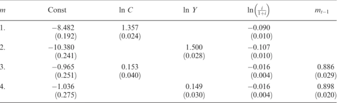
One of the earliest time series econometric attempts to estimate the impact of money was due to M. Friedman and Meiselman (1963). Their objective was to test whether monetary or fiscal policy was more important for the determination of nom-inalincome. To address this issue, they estimated the following equation:12
ytn1ytþpt¼ y0nþ
X
i¼0
aiAtiþ X
i¼0
bimtiþ X
i¼0
hiztiþut; ð1:1Þ
where yn denotes the log of nominal income, equal to the sum of the logs of output and the price level,Ais a measure of autonomous expenditures, andmis a monetary aggregate;zcan be thought of as a vector of other variables relevant for explaining nominal income fluctuations. Friedman and Meiselman reported finding a much more stable and statistically significant relationship between output and money than between output and their measure of autonomous expenditures. In general, they could not reject the hypothesis that theai coe‰cients were zero, while thebi coe‰-cients were always statistically significant.
The use of equations such as (1.1) for policy analysis was promoted by a number of economists at the Federal Reserve Bank of St. Louis, so regressions of nominal income on money are often calledSt. Louis equations (see L. Andersen and Jordon 1968; B. Friedman 1977a; Carlson 1978). Because the dependent variable is nominal income, the St. Louis approach does not address directly the question of how a money-induced change in nominal spending is split between a change in real output and a change in the price level. The impact of money on nominal income was esti-mated to be quite strong, and Andersen and Jordon (1968, 22) concluded, ‘‘Finding of a strong empirical relationship between economic activity and . . . monetary actions points to the conclusion that monetary actions can and should play a more promi-nent role in economic stabilization than they have up to now.’’13
12. This is not exactly correct; because Friedman and Meiselman included ‘‘autonomous’’ expenditures as an explanatory variable, they also used consumption as the dependent variable (basically, output minus autonomous expenditures). They also reported results for real variables as well as nominal ones. Following modern practice, (1.1) is expressed in terms of logs; Friedman and Meiselman estimated their equation in levels.
The original Friedman-Meiselman result generated responses by Modigliani and Ando (1976) and De Prano and Mayer (1965), among others. This debate empha-sized that an equation such as (1.1) is misspecified if mis endogenous. To illustrate the point with an extreme example, suppose that the central bank is able to manipu-late the money supply to o¤set almost perfectly shocks that would otherwise generate fluctuations in nominal income. In this case, yn would simply reflect the random control errors the central bank had failed to o¤set. As a result,mand yn might be completely uncorrelated, and a regression of yn on mwould not reveal that money actually played an important role in a¤ecting nominal income. If policy is able to re-spond to the factors generating the error termut, thenmt andut will be correlated, ordinary least-squares estimates of (1.1) will be inconsistent, and the resulting esti-mates will depend on the manner in which policy has induced a correlation between
u andm. Changes in policy that altered this correlation would also alter the least-squares regression estimates one would obtain in estimating (1.1).
1.3.2 Granger Causality
The St. Louis equation related nominal output to the past behavior of money. Simi-lar regressions employingrealoutput have also been used to investigate the connec-tion between real economic activity and money. In an important contribuconnec-tion, Sims (1972) introduced the notion ofGranger causalityinto the debate over the real e¤ects of money. A variableX is said to Granger-causeY if and only if lagged values ofX
have marginal predictive content in a forecasting equation forY. In practice, testing whether money Granger-causes output involves testing whether the ai coe‰cients equal zero in a regression of the form
yt¼y0þ X
i¼1
aimtiþ X
i¼1
biytiþ X
i¼1
ciztiþet; ð1:2Þ
where key issues involve the treatment of trends in output and money, the choice of lag lengths, and the set of other variables (represented byz) that are included in the equation.
with a time trend. Stock and Watson (1989) provided a systematic treatment of the trend specification in testing whether money Granger-causes real output. They con-cluded that money does help to predict future output (they actually used industrial production) even when prices and an interest rate are included.
A large literature has examined the value of monetary indicators in forecasting output. One interpretation of Sims’s finding was that including an interest rate reduces the apparent role of money because, at least in the United States, a short-term interest rate rather than the money supply provides a better measure of mone-tary policy actions (see chapter 11). B. Friedman and Kuttner (1992) and Bernanke and Blinder (1992), among others, looked at the role of alternative interest rate mea-sures in forecasting real output. Friedman and Kuttner examined the e¤ects of alter-native definitions of money and di¤erent sample periods and concluded that the relationship in the United States is unstable and deteriorated in the 1990s. Bernanke and Blinder found that the federal funds rate ‘‘dominates both money and the bill and bond rates in forecasting real variables.’’
Regressions of real output on money were also popularized by Barro (1977; 1978; 1979b) as a way of testing whether only unanticipated money matters for real out-put. By dividing money into anticipated and unanticipated components, Barro ob-tained results suggesting that only the unanticipated part a¤ects real variables (see also Barro and Rush 1980 and the critical comment by Small 1979). Subsequent work by Mishkin (1982) found a role for anticipated money as well. Cover (1992) employed a similar approach and found di¤erences in the impacts of positive and negative monetary shocks. Negative shocks were estimated to have significant e¤ects on output, whereas the e¤ect of positive shocks was usually small and statistically insignificant.
1.3.3 Policy Uses
Before reviewing other evidence on the e¤ects of money on output, it is useful to ask whether equations such as (1.2) can be used for policy purposes. That is, can a re-gression of this form be used to design a policy rule for setting the central bank’s pol-icy instrument? If it can, then the discussions of theoretical models that form the bulk of this book would be unnecessary, at least from the perspective of conducting mon-etary policy.
Suppose that the estimated relationship between output and money takes the form
yt¼y0þa0mtþa1mt1þc1ztþc2zt1þut: ð1:3Þ
mt¼
a1 a0mt1
c2
a0zt1þvt
¼p1mt1þp2zt1þvt; ð1:4Þ
where for simplicity it is assumed that the monetary authority’s forecast ofztis equal to zero. The termvtrepresents the control error experienced by the monetary author-ity in setting the money supply. Equation (1.4) represents a feedback rule for the money supply whose parameters are themselves determined by the estimated coe‰-cients in the equation for y. A key assumption is that the coe‰cients in (1.3) are in-dependent of the choice of the policy rule form. Substituting (1.4) into (1.3), output under the policy rule given in (1.4) would be equal to yt¼y0þc1ztþutþa0vt.
Notice that a policy rule has been derived using only knowledge of the policy ob-jective (minimizing the expected variance of output) and knowledge of the estimated coe‰cients in (1.3). No theory of how monetary policy actually a¤ects the economy was required. Sargent (1976) showed, however, that the use of (1.3) to derive a policy feedback rule may be inappropriate. To see why, suppose that real output actually depends only on unpredicted movements in the money supply; only surprises matter, with predicted changes in money simply being reflected in price level movements with no impact on output.14From (1.4), the unpredicted movement inmt is justvt, so let the true model for output be
yt¼y0þd0vtþd1ztþd2zt1þut: ð1:5Þ
Now from (1.4), vt ¼mt ðp1mt1þp2zt1Þ, so output can be expressed
equiva-lently as
yt¼y0þd0½mt ðp1mt1þp2zt1Þ þd1ztþd2zt1þut
¼y0þd0mtd0p1mt1þd1ztþ ðd2d0p2Þzt1þut; ð1:6Þ
which has exactly the same form as (1.3). Equation (1.3), which was initially inter-preted as consistent with a situation in which systematic feedback rules for monetary policy could a¤ect output, is observationally equivalent to (1.6), which was derived under the assumption that systematic policy had no e¤ect and only money surprises mattered. The two are observationally equivalent because the error term in both (1.3) and (1.6) is justut; both equations fit the data equally well.
A comparison of (1.3) and (1.6) reveals another important conclusion. The coe‰-cients of (1.6) are functions of the parameters in the policy rule (1.4). Thus, changes in the conduct of policy, interpreted to mean changes in the feedback rule
ters, will change the parameters estimated in an equation such as (1.6) (or in a St. Louis–type regression). This is an example of the Lucas (1976) critique: empirical relationships are unlikely to be invariant to changes in policy regimes.
Of course, as Sargent stressed, it may be that (1.3) is the true structure that re-mains invariant as policy changes. In this case, (1.5) will not be invariant to changes in policy. To demonstrate this point, note that (1.4) implies
mt¼ ð1p1LÞ1ðp2zt1þvtÞ;
where L is the lag operator.15Hence, we can write (1.3) as
yt¼y0þa0mtþa1mt1þc1ztþc2zt1þut
¼y0þa0ð1p1LÞ1ðp2zt1þvtÞ
þa1ð1p1LÞ1ðp2zt2þvt1Þ þc1ztþc2zt1þut
¼ ð1p1Þy0þp1yt1þa0vtþa1vt1þc1zt
þ ðc2þa0p2c1p1Þzt1þ ða1p2c2p1Þzt2þutp1ut1; ð1:7Þ
where output is now expressed as a function of lagged output, the zvariable, and money surprises (thevrealizations). If this were interpreted as a policy-invariant ex-pression, one would conclude that output is independent of any predictable or sys-tematic feedback rule for monetary policy; only unpredicted money appears to matter. Yet, under the hypothesis that (1.3) is the true invariant structure, changes in the policy rule (thep1coe‰cients) will cause the coe‰cients in (1.7) to change.
Note that starting with (1.5) and (1.4), one derives an expression for output that is observationally equivalent to (1.3). But starting with (1.3) and (1.4), one ends up with an expression for output that is not equivalent to (1.5); (1.7) contains lagged values of output,v, andu, and two lags ofz, whereas (1.5) contains only the contemporane-ous values of vand u and one lag of z. These di¤erences would allow one to dis-tinguish between the two, but they arise only because this example placed a priori restrictions on the lag lengths in (1.3) and (1.5). In general, one would not have the type of a priori information that would allow this.
The lesson from this simple example is that policy cannot be designed without a theory of how money a¤ects the economy. A theory should identify whether the coef-ficients in a specification of the form (1.3) or in a specification such as (1.5) will re-main invariant as policy changes. While output equations estimated over a single
policy regime may not allow the true structure to be identified, information from sev-eral policy regimes might succeed in doing so. If a policy regime change means that the coe‰cients in the policy rule (1.4) have changed, this would serve to identify whether an expression of the form (1.3) or one of the form (1.5) was policy-invariant.
1.3.4 The VAR Approach
Much of the understanding of the empirical e¤ects of monetary policy on real eco-nomic activity has come from the use of vector autoregression (VAR) frameworks. The use of VARs to estimate the impact of money on the economy was pioneered by Sims (1972; 1980). The development of the approach as it moved from bivariate (Sims 1972) to trivariate (Sims 1980) to larger and larger systems as well as the em-pirical findings the literature has produced were summarized by Leeper, Sims, and Zha (1996). Christiano, Eichenbaum, and Evans (1999) provided a thorough discus-sion of the use of VARs to estimate the impact of money, and they provided an ex-tensive list of references to work in this area.16
Suppose there is a bivariate system in which yt is the natural log of real output at time t, and xt is a candidate measure of monetary policy such as a measure of the money stock or a short-term market rate of interest.17The VAR system can be writ-ten as
yt
xt
¼AðLÞ yt1
xt1
þ uyt
uxt
; ð1:8Þ
whereAðLÞis a 22 matrix polynomial in the lag operator L, anduit is a timet se-rially independent innovation to theith variable. These innovations can be thought of as linear combinations of independently distributed shocks to output (eyt) and to policy (ext):
uyt
uxt
¼ eytþyext feytþext
¼ 1 y
f 1
eyt
ext
¼B eyt ext
: ð1:9Þ
The one-period-ahead error made in forecasting the policy variable xt is equal to
uxt, and since, from (1.9),uxt¼feytþext, these errors are caused by the exogenous output and policy disturbances eyt and ext. Letting Su denote the 22 variance-covariance matrix of theuit,Su¼BSeB0, where Seis the (diagonal) variance matrix of theeit.
16. Two references on the econometrics of VARs are Hamilton (1994) and Maddala (1992).
The random variableext represents the exogenous shock to policy. To determine the role of policy incausingmovements in output or other macroeconomic variables, one needs to estimate the e¤ect ofexon these variables. As long asf00, the inno-vation to the observed policy variablext will depend both on the shock to policyext and on the nonpolicy shockeyt; obtaining an estimate ofuxtdoes not provide a mea-sure of the policy shock unlessf¼0.
To make the example even more explicit, suppose the VAR system is
yt
xt
¼ a1 a2
0 0
yt1 xt1
þ uyt
uxt
; ð1:10Þ
with 0<a1 <1. Thenxt¼uxt, and yt ¼a1yt1þuytþa2uxt1, and one can write yt in moving average form as
yt¼
Xy
i¼0
a1iuytiþ
Xy
i¼0
a1ia2uxti1:
Estimating (1.10) yields estimates ofAðLÞandSu, and from these the e¤ects ofuxton
fyt;ytþ1;. . .gcan be calculated. If one interpreteduxas an exogenous policy distur-bance, then the implied response ofyt;ytþ1;. . .to a policy shock would be18
0;a2;a1a2;a21a2;. . .:
To estimate the impact of a policy shock on output, however, one needs to calcu-late the e¤ect onfyt;ytþ1;. . .gof a realization of the policy shockext. In terms of the true underlying structural disturbancesey andex, (1.9) implies
yt¼
Xy
i¼0
a1iðeytiþyextiÞ þ
Xy
i¼0
a1ia2ðexti1þfeyti1Þ
¼eytþ
Xy
i¼0
a1iða1þa2fÞeyti1þyextþ
Xy
i¼0
a1iða1yþa2Þexti1; ð1:11Þ
so the impulse response function giving the true response of yto the exogenous pol-icy shockexis
y;a1yþa2;a1ða1yþa2Þ;a12ða1yþa2Þ;. . .:
18. This represents the response to an nonorthogonalized innovation. The basic point, however, is that ify andfare nonzero, the underlying shocks are not identified, so the estimated response touxor to the
This response involves the elements ofAðLÞand the elements ofB. And whileAðLÞ can be estimated from (1.8),BandSeare not identified without further restrictions.19 Two basic approaches to solving this identification problem have been followed. The first imposes additional restrictions on the matrix B that links the observable VAR residuals to the underlying structural disturbances (see (1.9)). This approach was used by Sims (1972; 1988); Bernanke (1986); Walsh (1987); Bernanke and Blinder (1992); D. Gordon and Leeper (1994); and Bernanke and Mihov (1998), among others. If policy shocks a¤ect output with a lag, for example, the restriction that y¼0 would allow the other parameters of the model to be identified. The sec-ond approach achieves identification by imposing restrictions on the long-run e¤ects of the disturbances on observed variables. For example, the assumption of long-run neutrality of money would imply that a monetary policy shock (ex) has no long-run permanent e¤ect on output. In terms of the example that led to (1.11), long-long-run neutrality of the policy shock would imply thatyþ ða1yþa2Þ
P
ai
1 ¼0 ory¼ a2.
Examples of this approach include Blanchard and Watson (1986); Blanchard (1989); Blanchard and Quah (1989); Judd and Trehan (1989); Hutchison and Walsh (1992); and Galı´ (1992). The use of long-run restrictions is criticized by Faust and Leeper (1997).
In Sims (1972), the nominal money supply (M1) was treated as the measure of monetary policy (thexvariable), and policy shocks were identified by assuming that f¼0. This approach corresponds to the assumption that the money supply is prede-termined and that policy innovations are exogenous with respect to the nonpolicy innovations (see (1.9)). In this case,uxt¼ext, so from the fact thatuyt¼yextþeyt¼ yuxtþeyt, y can be estimated from the regression of the VAR residuals uyt on the VAR residuals uxt.20 This corresponds to a situation in which the policy variablex
does not respond contemporaneously to output shocks, perhaps because of informa-tion lags in formulating policy. However, if x depends contemporaneously on non-policy disturbances as well as non-policy shocks (f00), using uxt as an estimate ofext will compound the e¤ects ofeytonuxt with the e¤ects of policy actions.
An alternative approach seeks a policy measure for which y¼0 is a plausible as-sumption; this corresponds to the assumption that policy shocks have no contempo-raneous impact on output.21This type of restriction was imposed by Bernanke and Blinder (1992) and Bernanke and Mihov (1998). How reasonable such an tion might be clearly depends on the unit of observation. In annual data, the
assump-19. In this example, the three elements ofSu, the two variances and the covariance term, are functions of
the four unknown parameters,f,y, and the variances ofeyandex.