Journal of Economic Dynamics & Control 30 (2006) 2509–2531
Solving DSGE models with perturbation methods
and a change of variables
Jesu´s Ferna´ndez-Villaverde
a,, Juan F. Rubio-Ramı´rez
ba
Department of Economics, 160 McNeil Building, 3718 Locust Walk, University of Pennsylvania, Philadelphia, PA 19104, USA
b
Research Department, 1000 Peachtree St. NE, Federal Reserve Bank of Atlanta, Atlanta, GA 30309, USA
Received 24 November 2003; accepted 26 July 2005 Available online 1 December 2005
Abstract
This paper explores the application of the changes of variables technique to solve the stochastic neoclassical growth model. We use the method of Judd [2003. Perturbation methods with nonlinear changes of variables. Mimeo, Hoover Institution] to change variables in the computed policy functions that characterize the behavior of the economy. We report how the optimal change of variables reduces the average absolute Euler equation errors of the solution of the model by a factor of three. We also demonstrate how changes of variables correct for variations in the volatility of the economy even if we work with first-order policy functions and how we can keep a linear representation of the laws of motion of the model if we use a nearly optimal transformation. We discuss how to apply our results to estimate dynamic equilibrium economies.
r2005 Elsevier B.V. All rights reserved.
JEL classification:C63; C68; E37
Keywords:Dynamic equilibrium economies; Computational methods; Changes of variables; Linear and nonlinear solution methods
www.elsevier.com/locate/jedc
0165-1889/$ - see front matterr2005 Elsevier B.V. All rights reserved. doi:10.1016/j.jedc.2005.07.009
Corresponding author. Tel.: +1 219 898 15 04; fax: +1 215 573 20 57.
1. Introduction
This paper explores the application of the changes of variables technique to solve the stochastic neoclassical growth model. In an important recent contribution,Judd (2003) has provided formulas to apply changes of variables to the solutions of dynamic equilibrium economies obtained through the use of perturbation techniques. Standard perturbation methods provide a Taylor expansion of the policy functions that characterize the equilibrium of the economy in terms of the state variables of the model and a perturbation parameter. Judd’s derivations allow moving from this Taylor expansion to any other series in terms of nonlinear transformations of the state variables without the need to recompute the whole solution. This alternative approximation can be more accurate than the first because the change of variables induces nonlinearities that can help to track the true, but unknown, policy functions.
Judd’s results are important for several reasons. First, we often want to solve problems with a large number of state variables. Solving these models is difficult and costly. If we use perturbation methods, the number of derivatives required to compute the parameters of the Taylor expansion of the solution quickly explodes as we increase the order of the approximation (see Judd and Guu, 1997). One alternative strategy is to obtain a low-order expansion (a quadratic or even just a linear one) of the solution and move to a more accurate representation using a change of variables. Computing this low-order expansion and the change of variables is relatively inexpensive. Consequently, if we are able to select an adequate transformation, we can increase the accuracy of the solution enough to use our computation for quantitative analysis despite the high dimensionality of the state space.
Second, researchers frequently exploit approximated solutions to understand the analytics of dynamic equilibrium models. See, for example, the classical treatment of Hall (1971) or the recent work of Woodford (2003). Because of tractability considerations, those analyses limit themselves to first-order expansions. Clearly the usefulness of this approach depends on the quality of the approximation. Linear solutions, however, may perform poorly outside a small region around which we linearize. More importantly, as pointed out by Benhabib et al. (2001), linear solutions may even lead to incorrect findings regarding the existence and uniqueness of equilibrium. An optimal change of variables can address both increase the accuracy of the solution and avoid misleading local results while maintaining analytic tractability.
Motivated by the arguments above, this paper applies Judd’s methodology to the stochastic neoclassical growth model with leisure, the workhorse of dynamic macroeconomics. First, we derive a simple close-form relation between the parameters of the linear and the loglinear solution of the model. We extend this approach to a more general class of changes of variables: those that generate a policy function with a power function structure.
Second, we study the effects of that last particular class of changes of variable on the size of the Euler equation errors, i.e., those errors that appear in the optimality conditions of the agents because of the use of approximated solutions instead of the exact ones. We search for the optimal change of variable inside the class of power functions and report results for a benchmark calibration of the model and for alternative parameterizations. In that way, we study the performance of the procedure both for a nearly linear case (the benchmark calibration) and for more nonlinear cases (for example those with higher variance of the productivity shock). We find that, for the benchmark calibration, we reduce the average absolute Euler equation errors by a factor of three. This reduction makes the new approximated solution of the model competitive to much more involved nonlinear methods, such as finite elements or value function iteration, and to second-order perturbations.
Third, sensitivity analysis reveals how the change of variables corrects for movements in the exogenous variance of the economy through changes in the optimal values of the parameters of the transformation. This is true even for a first-order approximation to the policy function. In comparison, a standard linear (or loglinear) solution can only provide a certainty equivalent approximation. This property is a key advantage of our approach.
Fourth, sensitivity analysis also suggests that a particular change of variables that preserves the linearity of the solution is roughly optimal. We propose the use of this approximation because of two reasons. First, because as explained before, such linearity allows researchers to use the well understood toolbox of linear systems while achieving a level of accuracy not possible with the standard linearization. Second, because it facilitates taking the model to the data. In addition to being linear, we show how this quasi-optimal approximated solution also implies that the disturbances to the model are normally distributed. Consequently we can write the economy in a state-space form and use the Kalman filter to perform likelihood based inference.
Finally, we extend some of our results to the change of variables in second-order approximations. We show how a change of variables noticeably increases the accuracy of second-order approximations, even if those are already quite accurate when applied to the stochastic neoclassical growth model (seeAruoba et al., 2005, for details). Thus, our findings suggest that a second-order approximation with a change of variables is a highly attractive solution algorithm in terms of accuracy and simplicity.
between the linear and loglinear solution of the model. Section 6 explores the optimal change of variables within a flexible class of functions and reports a sensitivity analysis exercise. Section 7 discusses the use of the change of variables for estimation. Section 8 extends some of our results to second-order approximations. Section 9 concludes.
2. The stochastic neoclassical growth model
As mentioned above, we want to explore how the approximated solutions of the stochastic neoclassical growth model with leisure respond to nonlinear changes of variables. Three reason lead us to use this model. First, its popularity (directly or with small changes) to address a large number of questions (seeCooley, 1995) makes it a natural laboratory to explore the potential of Judd’s contribution. Second, because of this importance any analytical result regarding the (approximated) solution of the model is of interest in itself. Finally, since this model is nearly linear for a benchmark calibration, its use provides a particularly difficult laboratory for the change of variables approach: it bounds tightly the improvements we can obtain. We find important advantages of the technique even for this case. Consequently, the improvements coming from the change of variables approach are likely to be higher for more nonlinear economies.1
Since the model is well known (seeCooley and Prescott, 1995), we provide only the minimum exposition required to fix notation. There is a representative agent in the economy, whose preferences over stochastic sequences of consumptionct and leisure
1lt are representable by the utility function:
E0 X 1
t¼0
btUðct;ltÞ,
whereb2 ð0;1Þis the discount factor, E0is the conditional expectation operator and Uð;Þsatisfies the usual technical conditions.
There is one good in the economy, produced according to the aggregate production functionyt¼eztka
tl1ta wherekt is the aggregate capital stock, lt is the
aggregate labor input, and zt is a stochastic process representing random
technological progress. The technology follows a first-order processzt¼rzt1þt
withjrjo1 andtNð0;s2Þ. Capital evolves according to the law of motionktþ1¼
ð1dÞktþit where d is the depreciation rate and the economy must satisfy the
resource constraintyt¼ctþit.
Since both welfare theorems hold in this economy, we can solve directly for the social planner’s problem. We maximize the utility of the household subject to the production function, the evolution of the stochastic process, the law of motion for
capital, the resource constraint and some initial conditions for capital and the stochastic process.
The solution to this problem is fully characterized by the equilibrium conditions:
UcðtÞ ¼bEtfUcðtþ1Þð1þaeztþ1katþ11l
1a
tþ1 dÞg, UlðtÞ ¼ UcðtÞð1aÞeztkatl
a
t ,
ctþktþ1 ¼eztktal1taþ ð1dÞkt,
zt¼rzt1þet
given some initial capital and some initial value for the stochastic process for technology. The first equation is the standard Euler equation that relates current and future marginal utilities from consumption, the second one is the static first-order condition between labor and consumption, and the last two equations are the resource constraint of the economy and the law of motion of technology.
We solve for the equilibrium of this economy by finding two policy functions for next period’s capitalk0ð;;Þ, and laborlð;;Þ, which deliver the optimal choice of these controls as functions of the two state variables, capital and technology level, and the standard deviation of the innovation to the productivity levels. Using the budget constraint, cð;;Þ is a function ofkð;;Þandlð;;Þ. Note that we include the perturbation parameter as one explicit variable in the policy functions. That notation is convenient for the next section.
3. Solving the model using a perturbation approach
The system of equations listed above does not have a known analytical solution and we need to use a numerical method to solve it. In a series of seminal papers, Judd and coauthors (see Judd and Guu, 1992, 1997 and the textbook exposition in Judd, 1998, among others) have proposed to build a Taylor series expansion of the policy functions k0ð;;Þ, and lð;;Þ around the deterministic steady state where z¼0 ands¼0.
Ifk0 is equal to the value of the capital stock in the deterministic steady state and the policy function for labor is smooth, we can use a Taylor series to approximate this policy function aroundðk0;0;0Þwith the form
lpðk;z;sÞ ’ X
i;j;m
1
ðiþjþmÞ!
qiþjþmlpðk;z;sÞ
qkiqzjqsm
k
0;0;0
ðkk0Þizjsm,
where the subscript p stands for perturbation approximation. The policy function for next period capital will have an analogous representation.
The key idea of the perturbation methods is to set the parametersequal to zero (since in this case the model can be solved analytically) and to exploit
implicit-function theorems to pin down the unknown coefficients qiþjþmlpðk;z;sÞ
To do so, the first step is to linearize the equilibrium conditions of the model around the deterministic steady state, i.e. whens¼0. Then, we substitute capital and labor by the values given by the first-order expansion of the policy function and we solve for the unknown coefficients. The next step is to find the second-order expansion of the equilibrium conditions, again around the deterministic steady state, plug in the quadratic approximation of the policy function (evaluated with the first-order coefficients found before) and solve for the unknown second-first-order coefficients. We can iterate on this procedure as many times as desired to get an approximation of arbitrary order. For a more detailed explanation of these steps we refer the reader to Judd and Guu (1992).
Since perturbations only deliver an asymptotically locally correct expression for the policy functions, the accuracy achieved by the method may be poor either away from the deterministic steady state or when the order of the expansion is low.
Several routes have been proposed to correct for these problems. One, byCollard and Juillard (2001), uses bias correction to find the approximation of the solution around a more suitable point that the deterministic steady state. The second one, suggested byJudd (2003), changes the variables in terms of which we express the computed solution of the model. We review Judd’s proposal in next section.
4. The change of variables
The first-order perturbation solution to the stochastic neoclassical growth model can be written asfðxÞ ’fðaÞ þ ðxaÞf0ðaÞwherex¼ ðk;zÞare the variables of the expansion,a¼ ðk0;0Þis the deterministic steady-state value of those variables, and fðxÞ ¼ ðk0pðk;zÞ;lpðk;zÞÞis the unknown policy function of the model. Since the first-order perturbation solution does not depend ons, we drop it in this section to save on notation. We could easily consider higher order perturbation solutions, but we concentrate in the first-order approximations because of expositional reasons.
Let us now transform both the domain and the range of fðxÞ. Thus, to express some nonlinear function of fðxÞ, hðfðxÞÞ:R2!R2 as a polynomial in some transformation of x, YðxÞ:R2 !R2, we can use the Taylor series of gðyÞ ¼ hðfðXðyÞÞÞaroundb¼YðaÞ, whereXðyÞis the inverse ofYðxÞ.
Using the chain rule,Judd (2003)shows that
gðyÞ ¼hðfðXðyÞÞÞ ¼gðbÞ þGðbÞðYðxÞ bÞ, (1)
whereGðbÞis a 22 matrix, whose i;j entry is
Gij¼
X
m
qhi qfm
X
n
qfm qXn
qXn qyj .
From this expression we see that if we have computed the values of partial derivatives off, it is straightforward to find the value ofG.
5. A particular case: the loglinearization
Since the exact solution of the stochastic neoclassical growth model in the case of log utility andd¼1 is loglinear, many practitioners have favored the loglineariza-tion of the equilibrium condiloglineariza-tions of the model over linearizaloglineariza-tion in levels.2 This practice generates the natural question of finding the relation between the coefficients on both representations. We use (1) to get a simple closed-form answer to this question.
A first-order perturbation produces an approximated policy function in levels of the form3
ðk0k0Þ ¼a1ðkk0Þ þb1z,
ðll0Þ ¼c1ðkk0Þ þd1z,
wherekandzare the current states of the economy,l0is steady-state value for labor, and where, for convenience, we have dropped the subscript p where no ambiguity exists. As mentioned before, all the coefficients on s are zero in the first-order perturbation.
Analogously a loglinear approximation of the policy function will take the form
logk0logk0¼a2ðlogklogk0Þ þb2z, logllogl0¼c2ðlogklogk0Þ þd2z,
or in equivalent notation: b
k0¼a2kbþb2z, b
l¼c2kbþd2z,
wherebx¼logxlogx0is the percentage deviation of the variablexwith respect to its steady state.
How do we go from one approximation to the second one? First, we followJudd’s (2003)notation and write the linear system in levels as
k0
pðk;z;sÞ ¼f
1ðk;z;sÞ ¼f1ðk
0;0;0Þ þf11ðk0;0;0Þðkk0Þ þf12ðk0;0;0Þz,
lpðk;z;sÞ ¼f2ðk;z;sÞ ¼f2ðk0;0;0Þ þf12ðk0;0;0Þðkk0Þ þf22ðk0;0;0Þz,
where
f1ðk0;0;0Þ ¼k0 f11ðk0;0;0Þ ¼a1 f12ðk0;0;0Þ ¼b1 f2ðk0;0;0Þ ¼l0 f21ðk0;0;0Þ ¼c1 f22ðk0;0;0Þ ¼d1
2
The wisdom of this practice is disputable. See for example,Dotsey and Mao (1992)andAruoba et al. (2005)for two papers that find that linearization performs better than loglinearization.
Second, we propose the changes of variables:
h1¼logf1 Y1ðxÞ ¼logx1 X1 ¼expy1
h2¼logf2 Y2¼x2 X2¼y2
Judd’s (2003)formulas for this particular example imply
logk0ðlogk;zÞ
loglðlogk;zÞ !
¼gðlogk;zÞ ¼
logf1ðk0;0;0Þ
logf2ðk0;0;0Þ !
þ
1 k0
f11ðk0;0;0Þk0 1 k0
f12ðk0;0;0Þ
1 l0
f21ðk0;0;0Þk0 1 l0
f22ðk0;0;0Þ 0 B B B @ 1 C C C A
logklogk0
z
! ,
and thus
logk0logk0¼f11ðk0;0;0Þðlogklogk0Þ þ 1 k0
f12ðk0;0;0Þz,
logllogl0¼ k0
l0
f21ðk0;0;0Þðlogklogk0Þ þ 1 l0
f22ðk0;0;0Þz.
By equating coefficients we obtain a simple closed-form relation between the parameters of both representations:4
a2¼a1 b2¼k10b1
c2¼kl00c1 d2¼l10d1
Note that we have not used any assumption on the utility or production functions except that they satisfy the general technical conditions of the neoclassical growth
4An alternative heuristic argument that delivers the same result is as follows. Take the system
ðk0
k0Þ ¼a1ðkk0Þ þb1z,
ðll0Þ ¼c1ðkk0Þ þd1z.
and divide on both sides by the steady-state value of the control variable: k0k
0 k0
¼a1 kk0
k0
þ 1
k0 b1z,
ll0 l0
¼c1 kk0
l0
þ1
l0 d1z.
Sincex0x0
model. Also, moving from one coefficient set to the other one is an operation that only involvesk0andl0, values that we need to find anyway to compute the linearized version in levels. Therefore, once you have the linear solution, obtaining the loglinear one is immediate.
6. The optimal change of variables
In the last section, we showed how to find a loglinear approximation to the solution of the neoclassical growth model directly from its linear representation. Now, we generalize our result to encompass the relationship between any power function approximation and the linear coefficients of the policy function. Also, we search for the optimal change of variable inside this class of power functions and we report how the Euler equation errors improve with respect to the linear representation.
6.1. A power function transformation
Before, we argued that some practitioners have defended the use of loglineariza-tions to capture some of the nonlinearities in the data. This practice can be pushed one step ahead. We can generalize the log function into a general class of power function of the form
k0pðk;z;g;z;mÞgk0g¼a3ðkzkz0Þ þb3z, lpðk;z;g;z;mÞmlm0 ¼c3ðkzkz0Þ þd3z.
This class of functions is attractive because it provides a lot of flexibility in shapes with only three free parameters, while including the log transformation as the limit case when the coefficientsg,z, andmtend to zero. A similar power function with only two parameters is proposed byJudd (2003) in a growth model without leisure and stochastic perturbations. His finding of notable improvements in the accuracy of the solution when he optimally selects the value of these parameters is suggestive of the advantages of using this parametric family.
The changes of variables for this family of functions are given by
h1¼ ðf1Þg Y1¼ ðx1Þz
X1¼ ðy1Þ
1
z
h2¼ ðf1Þm Y2¼x2 X2¼y2
Following the same reasoning than in the previous section, we derive a form for the system in term of the original coefficients:
k0pðk;z;g;z;mÞgkg0¼g zk
gz
0 a1ðkzkz0Þ þgk
g1
0 b1z,
lpðk;z;g;z;mÞmlm0 ¼ m z l
m1
0 k
1z
0 c1ðkzkz0Þ þml
m1
Therefore, the relation of between the new and the old coefficients is again simple to compute:
a3¼gzkgz0 a1 b3¼gkg0 1b1
c3¼mzl m1
0 k
1z
0 c1 d3¼mlm0 1d1
6.2. Searching for the optimal transformation
One difference between the transformation from linear into a loglinear solution and the current transformation into a power law is that we have three free parametersg,z, andm. How do we select optimal values for those?
A reasonable criterion is to select them in order to improve the accuracy of the solution of the model. This desideratum raises a question. How do we measure this accuracy, conditional on the fact that we do not know the true solution of the model? Judd and Guu (1992) solves this problem evaluating the normalized Euler equation errors (see alsoSantos, 2000;Den Haan and Marcet, 1994). Note that in our model intertemporal optimality implies that
UcðtÞ ¼bEtfUcðtþ1Þð1þaeztþ1katþ11l
1a
tþ1 dÞg. (2) Since the solutions are not exact, condition (2) will not hold exactly when evaluated using the computed decision rules. Instead, for any choice of g, z, and m and its associated policy rulesk0pð;;g;z;mÞandlpð;;g;z;mÞ, we can define the normalized absolute value Euler equation errors as
EEðk;z;XÞ ¼ 1ðU
1
c ðEtUcðtþ1ÞbR0ðk;z;XÞ;lpðk;z;XÞÞÞ cpðk;z;XÞ
, (3)
whereX¼ ðg;z;mÞ,R0ðk;z;XÞ ¼ ð1þaeztþ1k0ðk;z;XÞa1l0ðk;z;XÞ1adÞis the gross
return on capital next period, and where we have used the static optimality condition to substitute labor by its optimal choice.
This expression evaluates the (unit free) error in the Euler equation measured as a fraction ofcpð;;XÞas a function of the current statesk, and z, and the change of variables defined byg,z, andm.Judd and Guu (1997)interpret this function as the mistake, in dollars, incurred by each dollar spent. For example,EEðk;z;XÞ ¼0:01 means that the consumer makes a 1 dollar mistake for each 100 dollar spent.
Our criterion is to select values ofXthat minimize the Euler error function. But here we face another problem. This function depends not only on the parametersX, but also on the values of the state variables. How do we eliminate that dependency? Do we minimize the Euler equation error at one particular point of the state space like the deterministic steady state? Do we minimize instead some weighted mean of it?
A first choice could be the criterion minX
R
particular point: we would want to nail down the Euler equation errors for those parts of the stationary distribution where most of the action would happen, while we would care less about accuracy in those points not frequently visited. The difficulty of the criterion is that we do not know that true stationary distribution (at least for capital) before we find the policy functions of the model.
To avoid this difficulty, we could solve a fixed-point problem where we get some approximation of the model, compute a stationary distribution, resolve the minimization problem, find the new stationary distribution, and continue until convergence. This approach faces two problems. First, it would be expensive in computing time. Second, there is no known theory result that guarantees the convergence of such iteration to the right set of values for the parameters of the transformation.
Given the difficulties of the previous approach, we follow a simpler strategy. Inspired by collocation schemes in projection methods, we minimize the Euler equation errors over a grid of points ofkandz:
min
X SEEðXÞ ¼minX
X
k;z
EEðk;z;XÞ. (4)
Setting this grid around the deterministic steady state (big enough to be representative of the stationary distribution of the economy but not too wide to avoid minimization over regions infrequently visited) may achieve our desire goal of improving the accuracy of the solution.5
Inspection of (4) reveals that this problem depends on the values of the structural parameters of the model, i.e. those describing preferences and technology. Consequently, we need to take a stand on those before we can report any result. We will calibrate of the model to match basic observations of the US economy following the common strategy in macroeconomics and, later, perform sensitivity analysis. Hence, we evaluate how much accuracy we win in a ‘real life’ situation by applying our change of variables and how confident we are in our results.
First we select as our utility function the CRRA form
ðcy
tð1ltÞ1yÞ1t
1t ,
wheretdetermines the elasticity of intertemporal substitution and ycontrols labor supply. Then we pick the benchmark calibration values as follows. The discount factor b¼0:99 matches an annual interest rate of 4 percent. The parameter that governs risk aversiont¼2 is a common choice in the literature. y¼0:36 matches
5
the microeconomic evidence of labor supply to 0.31 of available time in the deterministic steady state. We seta¼0:4 to match labor share of national income (after the adjustments to National Income and Product Accounts suggested by Cooley and Prescott, 1995). The depreciation rate d¼0:0196 fixes the investment/ output ratio and r¼0:95 and s¼0:007 follow the stochastic properties of the Solow residual of the US economy.Table 1 summarizes the discussion. Later, we discuss the sensitivity of our results to change in parameter values.
Also, we need to define the set of points forkand zover which we are going to sum the normalized absolute value Euler equation errors. We define a grid of 21 capital points covering30 percent above and below the steady-state capital and a grid of 21 productivity points using Tauchen (1986) procedure. Using highly accurate nonlinear methods, we computed that our grid covers over 99 percent of the stationary distribution of the economy.
We report our main findings inTable 2. The last entry of the second row is the value of SEEð1;1;1Þ, i.e., for the linear approximation for the Benchmark calibration. The third row is the solution to problem (4).
We highlight several points. First, the parametersg andzare both close to one suggesting that the nonlinearities in capital are of little importance (although not totally absent, sinceSEEðXÞsuffers when we impose that both parameters are equal to one). That result is confirmed by inspecting the nearly linear policy functions for capital found by very accurate but expensive nonlinear methods (see the results reported inAruoba et al., 2005). Second,mis far away from zero. The interpretation is that the labor supply function is much more nonlinear in capital and allowing the policy function to capture that behavior increases the accuracy of the solution.
The last column of the Table 2 shows that the optimal change of variables improves the average absolute value Euler equation error by a factor of around three. This means that, for each mistake of three dollars made using the linear approximation, the consumer would only have made a one dollar mistake using the
Table 1
Calibrated parameters
Parameter b t y a d r s
Value 0.99 2.0 0.36 0.4 0.02 0.95 0.007
Table 2
Euler equation errors
g z m SEEðXÞ
1 1 1 0.0856279
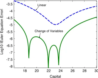
optimal change of variable, a sizeable (but not dramatic) improvement in accuracy. This same result is shown inFig. 1, where we plot the decimal log of the absolute Euler equation errors at z¼0 for the ordinary linear solution and the optimal change of variable. The use of decimal logs eases the reading of the graph. A value of
3 in the vertical axis represents an error of 1 dollar out of each 1000 dollars, a value of4 an error of 1 dollar out of each 10,000 dollars and so on. InFig. 1, we observe that when only one dimension is considered, the optimal change of variable can improve Euler equation errors from around 1 dollar every 10,000 dollars to 1 dollar every 1,000,000 dollars (an even more in some points).
We explore how the optimal change of variable compares with other more conventional nonlinear methods in terms of accuracy. In Fig. 2, we compare the Euler equation errors generated by the optimal change of variables with the Euler errors implied by different linear and nonlinear solution methods (seeAruoba et al., 2005, for details about the other methods). The graph shows how the optimal change of variable solution pushes a first-order approximation to the accuracy level delivered by the finite elements method for most of the interval. If we consider the computational and coding costs of implementing the finite elements method, this result provides strong evidence in favor of using a combination of linear solution and optimal change of variable as a solution method for macroeconomic models. Also, the new approximation is roughly comparable in terms of accuracy with a second-order approximation of the policy function defended bySims (2002a)and Schmitt-Grohe´ and Uribe (2004).
We finish by pointing out how the change of variables might have the additional advantage of suffering less often from the problem of explosive behavior of simulations present in the second and higher order perturbations. This explosive behavior appears because of the presence of higher order terms in the perturbation solution. Sometimes, the productivity shocks are so big that the high powers of the
18 20 22 24 26 28 30
-8 -7.5 -7 -6.5 -6 -5.5 -5 -4.5 -4 -3.5
Capital
Log10 |Euler Equation Error|
Linear
Change of Variables
solution send the path of capital outside the stable manifold. For example,Aruoba et al. (2005)find that, for a model like the one studied in this paper, up to 4 percent of the simulations led to explosive paths when they use a fifth-order approximation. There are two solutions to this problem. First, those explosive simulation can be eliminated from the computation. However, there is a certain degree of arbitrariness in the definition of when a path becomes explosive. Second, Kim et al. (2003) propose an algorithm that always produces stationary second-order accurate dynamics whenever the first-order dynamics are stable.
The change of variables suffers less from the problem of explosive paths because it raises the state variables at lower powers. In our application, the powers in the policy function for capital (the one exposed to explosive behavior) vary from 0.97 to 1.24. These lower powers stop most explosive paths. An example can be seen inFig. 3. We draw two simulated time series of capital for our model withs¼0:56 (the higher variance of productivity shocks needed to show more clearly the presence of explosive paths). The first line plots the series of capital induced by a fifth-order perturbation. The second line plots the series of capital for the optimal change of variables. From this figure we can see how for the first 150 periods, both series are close. However, around period 175 they separate and, after a few periods, the simulation from the fifth-order explodes while the simulation from the optimal change of variables, despite also showing an increase in the amount of capital, stays within the stable manifold.
6.3. Sensitivity analysis
How does the solution to (4) depend on the chosen calibration? Are the optimal parameters values inXrobust to changes in the values of the structural parameters of the economy?
18 20 22 24 26 28 30
-9 -8 -7 -6 -5 -4 -3
Capital
Log10 |Euler Equation Error|
Linear
5th Order Perturbation
FEM
2nd Order Perturbation Change of Variables
Loglinear
We analyzed in detail how the optimal change of variables depends on the different parameter values. We report only a sample of our findings with the most interesting results. We discuss the effect of changes in the share of capitala(Table 3), in the parameter governing the intertemporal elasticity of substitution t(Table 4), and in the standard deviation of the technology shocks(Table 5).
In Table 3 we see how gand zstay close to 1 although some variation in their values is induced by the changes in the capital share. On the other hand,mchanges from 0.9 to 2.47. Interestingly, all of this change happens when we move from a¼0:2 to a¼0:4. This drastic change is due to the fact that the steepness of the marginal productivity of capital changes rapidly for values ofa around this range. Table 4shows the results are more robust with respect to changes int. This finding is important because it documents that the change of variables has a difficult time to capture the effects of large risk aversion.
Table 5shows the effects of changingsfrom its benchmark case of 0.07 to 0.014, 0.028, and 0.056. Here we observe more action:gandzmove a bit andmgoes all the way down from 2.48 to 0.78. Higher variance of the productivity shock increases the
0 50 100 150 200 250
5 10 15 20 25 30 35 40 45 50
Time
Capital
Fifth-Order Perturbation
Optimal Change of Variables
Fig. 3. Time series of capital.
Table 3
Optimal parameters for differentas
a g z m
0.2 1.05064 1.06714 0.90284
0.4 0.98653 0.99167 2.47856
0.6 0.97704 0.97734 2.47796
precautionary motive for consumers and induces stronger nonlinearities in the computed policy functions of the model.
The variation in optimal parameter values is a significant result. It shows how the change of variables allows for a correction based on the level of uncertainty existing in the economy. This correction cannot be achieved by linearization approach since that strategy produces a certainty equivalent approximation. The ability to adapt to different volatilities while keeping a first-order structure in the solution is a key advantage of the change of variables procedure.
We conclude from our sensitivity analysis that the choices of optimal parameter values ofg,z, andm are stable across very different parameterizations and that the only relevant change is for the value ofmwhen we vary capital share or the variance of the technology shock.
6.4. A linear representation of the solution
Our previous findings motivate the following observation. Since g and z are roughly equal across different parameterizations, we can confine ourselves to the two parameter transformation:
k0gkg0¼a3ðkgkg0Þ þb3z, lmlm0¼c3ðkgkg0Þ þd3z,
while keeping nearly all the same level of accuracy obtained by the more general case.
To illustrate our point we plot the Euler Equation error for this restricted optimal case in Fig. 4 with g¼1:11498 and m¼0:948448. Comparing with the optimal change we can appreciate how we keep nearly all the increment in accuracy. More formally theSEEðXÞmoves now to 0.0420616.
Table 4
Optimal parameters for differentts
t g z m
4 1.02752 1.03275 2.47922
10 1.04207 1.04671 2.47830
50 1.01138 1.01638 2.47820
Table 5
Optimal parameters for differentss
s g z m
0.014 0.98140 0.98766 2.47753
0.028 1.04804 1.05265 1.73209
The proposed two parameter transformation is very convenient because if we definekb¼kgkg0 andbl¼lmlm0 we can rewrite the equations as
b
k0¼a3kbþb3z, b
l¼c3kbþd3z
producing a linear system of difference equations.
This implies that we can study the neoclassical growth model (or a similar dynamic equilibrium economy) in the following way. First, we find the equilibrium conditions of the economy. Second, we linearize them (or loglinearize if it is easier) and solve the resulting problem using standard methods. Third, we transform the variables (leaving the parameters of the transformation undetermined until the final numerical analysis) and study the qualitative properties of the new system using standard techniques. If the transformation captures some part of the nonlinearities of the problem we may be able to avoid the problems singled out byBenhabib et al. (2001). Fourth, if we want to study the quantitative behavior of the economy we pick values for the parameters according to (4) and simulate the economy using the transformed system.
7. Changes of variables for estimation
Often, dynamic equilibrium models can be written in a state-space representation, with a transition equation that determines the law of motion for the states and a measurement equation that relates states and observables. It is well known that models with this representation are easily estimated using the Kalman Filter (see Harvey, 1989).
18 20 22 24 26 28 30 -8
-7.5 -7 -6.5 -6 -5.5 -5 -4.5 -4 -3.5
Capital
Log10 |Euler Equation Error|
Linear
Optimal Change
Restricted Optimal Change
Consequently, a common practice to take the stochastic neoclassical growth model to the data has been to linearize the equilibrium conditions in levels or in logs around the steady state to get a transition and a measurement equation, use the Kalman recursion to evaluate the implied likelihood, and then, either to maximize it (in a classical perspective) or to draw from the posterior (in a Bayesian approach). In this subsection we propose a variation of this strategy. Since in our computations we find thatgandzare roughly equal, we propose to use
b
k0¼a3kbþb3z (5)
in the transition equation and (possibly)
bl¼c3kbþd3z (6)
in the measurement equation, wherekb¼kgkg0andbl¼lmlm0, instead of the usual linear or loglinear relations. Since both equations are still linear in the transformed variables, the conditional distributions of the variables is normal and we can use the Kalman Filter to evaluate the likelihood. The only difference now will be that, in addition to depend on the structural parameters of the model, the likelihood will also be a function of the parametersgandm.
This approach allows us to keep a linear representation suitable for efficient estimation while capturing an important part of the nonlinearities of the model and avoiding the use of expensive simulation methods like a particle filter.
To illustrate the potentiality of our proposal, we proceed as follows. First, we generate 200 observation of ‘artificial’ data for hours worked,lT¼ fltg200t¼1, from the stochastic neoclassical growth model that we presented above. We solved the model using the finite elements method as described inAruoba et al. (2005)to generate an artificial sample with nonlinearities. Second, we compute the likelihood function implied by the approximated solution (5) and (6), where g and z are chosen to minimize the problem (4). For comparison purposes, we compute the likelihood implied by the loglinear solution. We evaluate both likelihood functions at the same parameter values that we use to generate the ‘artificial’ data for hours worked.
A simple procedure to compare both solutions is to implement a likelihood ratio test. This test will tells which of the two models, the one represented by (5) and (6) or the usual loglinear model, fits the data better.
We compute the likelihood ratio test for two different points in the parameter space. First, we use the parameter values described in our benchmark calibration. Second, we also consider a more extreme case wheret¼50 ands¼0:035, while we maintain the value of the rest of the parameters to the values reported inTable 1. We recognize that the extreme case (high risk aversion/high variance) is not realistic, but it allows us to easily consider a very nonlinear case.6
The likelihood ratio is defined by
bl¼L
RðlTjY;g¼1;m¼1Þ
LUðlTjY;g;mÞ ,
where,Y¼ ðb;s;t;y;a;d;rÞ,LUðlTjY;g;
mÞstands for the likelihood of the ‘unrest-ricted model’, wheregandzare chosen to minimize (4), andLRðlTjY;g¼1;m¼1Þ stands for the likelihood of the ‘restricted model’, wheregandzare restricted to be equal to one. Under the null hypothesis thatg¼1 andm¼1,2 logblis distributed as aw2with two degrees of freedom (corresponding to the two restrictions).Table 6 reports the values of2 logblfor the two different choices of the parameter values. In the benchmark case, the value of the statistic is 3.52. The statistic clearly indicates that the optimal change of variables fits the data better. However, the improvement in fit is not dramatic and the statistic is only significant at the 20 percent level. The result is not surprising, since in the benchmark case the model is almost linear.
In the extreme case, the results are overwhelming in favor of the solution described by (5) and (6). The improvement in fit is so high that the value of the statistic is 163.06, with significance at any tabulated value. This example shows how, when the data is generated from a very nonlinear model, the change of variables approach is able to capture those linearities and fits the data much better than the typical loglinear model.
The large differences in likelihoods corroborate a finding byFerna´ndez-Villaverde et al. (2005). The authors document how second-order approximation errors in the policy function, which almost always are ignored by researchers when estimating dynamic equilibrium models, have first-order effects on the likelihood function. The authors show that the approximated likelihood function converges at the same rate as the approximated policy function. However, the error in the approximated likelihood function gets compounded with the size of the sample. Therefore, period by period, small errors in the policy function accumulate at the same rate at which the sample size grows.
The results of Ferna´ndez-Villaverde et al. (2005) can also be interpreted as suggesting the need for highly accurate solution methods for dynamic equilibrium models if we want to estimate them. Since the change of variables substantially reduces the approximation errors in the policy function for a trivial computational cost, the method in this paper presents itself as a very attractive alternative for applied researchers.
8. The change of variables for the second-order approximation
FollowingJudd and Guu (1992, 1997), recent work bySchmitt-Grohe´ and Uribe (2004)and bySims (2002a)has popularized the use of second-order approximations to the solution of dynamic equilibrium models. Consequently, it is of interest to show how the change of variables applies to this second-order approximations. Table 6
Likelihood ratio test
Case Benchmark Extreme
The second-order perturbation solution to the stochastic neoclassical growth model can be written as fðxÞ ’fðaÞ þ ðxaÞf0ðaÞ þ12ðxaÞf00ðaÞðxaÞ0 where x¼ ðk;z;sÞ are the variables of the expansion, a¼ ðk0;0;0Þ is the deterministic steady-state value of those variables, and fðxÞ ¼ ðk0pðk;z;sÞ;lpðk;z;sÞÞ is the unknown policy function of the model. Note that, since it this case the policy functions depend on s, we add this parameter to the state variables of the system.
As before, we transform both the domain and the range offðxÞ. Thus, to express some nonlinear function of fðxÞ, hðfðxÞÞ:R2!R2 as a polynomial in some transformation of x, YðxÞ:R3 !R3, we can use the Taylor series of gðyÞ ¼ hðfðXðyÞÞÞaroundb¼YðaÞ, whereXðyÞis the inverse ofYðxÞ.
Using the chain rule, it can be shown that
giðyÞ ¼hiðfðXðyÞÞÞ ¼giðbÞ þGiðbÞðYðxÞ bÞ þ12ðYðxÞ bÞ0HiðbÞðYðxÞ bÞ
fori¼1;2 whereGiðbÞis a 13 matrix, whosejentry is
Gij¼qh
i
qfi qfi qXi
qXi qyj
andHiðbÞis a 33 matrix, whose s;jentry is
Hisj¼qG
i s
qyj
fori¼1;2 ands;j¼1;2;3. As for the linear case, if we have computed the values of f0, then it is straightforward to find the value ofG.
8.1. A power function transformation
Now, we apply our previous derivations to the second-order perturbation of the neoclassical growth model:
k0pðk;z;g;z;mÞ k0¼a1ðkk0Þ þb1zþc1ðkk0Þ2þd1z2þe1s2þf1ðkk0Þz, lpðk;z;g;z;mÞ l0¼a2ðkk0Þ þb2zþc2ðkk0Þ2þd2z2þe2s2þf2ðkk0Þz.
Following our previous framework for the linear approximation, we consider the power transformation for the second-order perturbation of the class:
k0pðk;z;g;z;mÞ
g
kg0¼a3ðkzkz0Þ þb3zþc3ðkzkz0Þ 2
þd3z2þe3s2þf3ðk
z
kz0Þz,
lpðk;z;g;z;mÞmlm0¼a4ðkzkz0Þ þb4zþc4ðkzkz0Þ 2
þd4z2þe4s2þf4ðk
z kz0Þz.
The changes of variables for this family of functions are given byh1¼ ðf1Þg and h2¼ ðf1Þm, while
Y1¼ ðx1Þz Y
2 ¼x2 Y2 ¼x2
X1 ¼ ðy1Þ
1
We derive a form for the system in term of the original coefficients:
k0pðk;z;g;z;mÞgkg0¼g zk
gz
0 a1ðk
zkz
0Þ þgk
g1
0 b1z,
lpðk;z;g;z;mÞmlm0 ¼ m z l
m1
0 k
1z
0 c1ðkzkz0Þ þml
m1
0 d1z.
Therefore, the relation of between the new and the old coefficients is simple to compute:
a3¼gzkgz0 a1 a4¼mzl
m1
0 k
1z
0 a2
b3¼gkg0 1b1 b4¼mlm0 1b2
c3¼zg2 k
g2z
0 ðc1k0þa1ð1þa1ðg1Þ zÞÞ c4¼zm2 k
12z
0 l
g2
0 ðc1k0l0þa2
ðl0ð1zÞ þk0a2ðm1ÞÞÞ
d3¼gk02þgðd1k0þb21ðg1ÞÞ d4¼ml02þmðd2l0þb22ðm1ÞÞ
e3¼e1kg0 1g e4¼e2lm0 1m
f3¼gzk
gz1
0 ðf1k0þa1b1ðg1ÞÞ f4¼mzk
1z
0 l
2þm 0
ðf2l0þa2b2ðm1ÞÞ
8.2. Results
As in the linear case, we determine the coefficientsg,z, andmin order to minimize the sum of the Euler Errors, as defined by problem (4).Table 7presents the results from such exercise.
We highlight two findings. First, the change of variables reduces the sum of Euler Errors by a 38 percent, a substantial improvement in terms of accuracy given the trivial computation cost of the change of variables. Second, this increase in accuracy is on top of the already good performance in terms of accuracy of the second-order perturbation when applied to the neoclassical growth model as documented byAruoba et al. (2005). Consequently, our results suggest that a second-order approximation with a change of
Table 7
Euler equation errors
g z m SEEðXÞ
1 1 1 0.00044651
variables is a highly attractive solution procedure for dynamic equilibrium models both in terms of accuracy and simplicity of computation.
Unfortunately, the second-order approximation implies the loss of linearity of the system, even with a restricted optimal transformation. This lack of linearity prevent us for using the Kalman filter for estimation purposes. Ferna´ndez-Villaverde and Rubio-Ramı´rez (2004)show how to apply the particle filter to estimate a nonlinear model similar to the one described here.
9. Concluding remarks
This paper has explored the effects of changes of variables in the policy function of the stochastic neoclassical growth model as first proposed byJudd (2003). We have shown how this change of variables helps to obtain a more accurate solution to the model both for analytical and empirical applications.
The procedure proposed is conceptually straightforward and simple to implement, yet powerful enough to substantially increase the quality of our solution to the neoclassical growth model. For our benchmark calibration the average Euler equation error is divided by three and the new policy function has a performance comparable with the policy functions generated by fully nonlinear methods. In addition, within the class of power functions considered in the paper, the optimal change of variables allows us to keep a linear structure of the model. This finding is useful for analytical and estimation purposes. Several questions remain to be explored further. What is the optimal class of parametric families to use in the changes of variables? Are those optimal families robust across different dynamic equilibrium models? How big is the increment in accuracy in other types of models of interest to macroeconomists? How much do we gain in accuracy of our estimates by using a transformed linear state space representation of the model? We plan to address these issues in our future research.
Acknowledgements
This paper circulated under the title: ‘Some Results on the Solution of the Neoclassical Growth Model’. We thank Dirk Krueger and participants at SITE 2003 for useful comments and Kenneth Judd for pointing out this line of research to us. Jesu´s Ferna´ndez-Villaverde thanks the NSF for financial support under the Project SES-0338997. Beyond the usual disclaimer, we notice that any views expressed herein are those of the authors and not necessarily those of the Federal Reserve Bank of Atlanta or of the Federal Reserve System.
References
Benhabib, J., Schmitt-Grohe´, S., Uribe, M., 2001. The perils of Taylor rules. Journal of Economic Theory 96, 40–69.
Blanchard, O.J., Kahn, C.M., 1980. The solution of linear difference models under linear expectations. Econometrica 48, 1305–1311.
Collard, F., Juillard, M., 2001. Perturbation methods for rational expectations models. Mimeo, CEPREMAP.
Cooley, T.F., 1995. Frontiers of Business Cycle Research. Princeton University Press, Princeton. Cooley, T.F., Prescott, E.C., 1995. Economic growth and business cycles. In: Cooley, T.F. (Ed.), Frontiers
of Business Cycle Research. Princeton University Press, Princeton, pp. 1–38.
Den Haan, W.J., Marcet, A., 1994. Accuracy in simulations. Review of Economic Studies 61, 3–17. Dotsey, M., Mao, C., 1992. How well do linear approximation methods work? The production tax case.
Journal of Monetary Economics 29, 25–58.
Ferna´ndez-Villaverde, J., Rubio-Ramı´rez, J.F., 2004. Estimating macroeconomic models: a likelihood approach. Federal Reserve Bank of Atlanta Working Paper 2004-1.
Ferna´ndez-Villaverde, J., Rubio-Ramı´rez, J.F., Santos, M., 2005. Convergence properties of the likelihood of computed dynamic models. Econometrica, forthcoming.
Hall, R., 1971. The dynamic effects of fiscal policy in an economy with foresight. Review of Economic Studies 38, 229–244.
Harvey, A.C., 1989. Forecasting, Structural Time Series Models, and the Kalman Filter. Cambridge University Press, Cambridge.
Judd, K.L., 1998. Numerical Methods in Economics. MIT Press, Cambridge.
Judd, K.L., 2003. Perturbation methods with nonlinear changes of variables. Mimeo, Hoover Institution. Judd, K.L., Guu, S.M., 1992. Perturbation solution methods for economic growth model. In: Varian, H.
(Ed.), Economic and Financial Modelling in Mathematica. Springer, New York Inc., New York. Judd, K.L., Guu, S.M., 1997. Asymptotic methods for aggregate growth models. Journal of Economic
Dynamics and Control 21, 1025–1042.
Kim, J., Kim, S., Schaumburg, E., Sims, C.A., 2003. Calculating and using second-order accurate solutions of discrete time dynamic equilibrium models. Mimeo, Princeton University.
King, R.G., Plosser, C.I., Rebelo, S.T., 2002. Production, growth and business cycles: technical appendix. Computational Economics 20, 87–116.
Klein, P., 2000. Using the generalized Schur form to solve a multivariate linear rational expectations model. Journal of Economic Dynamics and Control 24, 1405–1423.
Kydland, F.E., Prescott, E.C., 1982. Time to build and aggregate fluctuations. Econometrica 50, 1345–1370.
Santos, M.S., 2000. Accuracy of numerical solutions using the Euler equation residuals. Econometrica 68, 1377–1402.
Schmitt-Grohe´, S., Uribe, M., 2004. Solving dynamic general equilibrium models using a second-order approximation to the policy function. Journal of Economic Dynamics and Control 28, 755–775. Sims, C.A., 2002a. Second-order accurate solution of discrete time dynamic equilibrium models. Mimeo,
Princeton University.
Sims, C.A., 2002b. Solving linear rational expectations models. Computational Economics 20, 1–20. Tauchen, G., 1986. Finite state Markov-chain approximations to univariate and vector autoregressions.
Economics Letters 20, 177–181.
Uhlig, H., 1999. A toolkit for analyzing nonlinear dynamic stochastic models easily. In: Marimo´n, R., Scott, A. (Eds.), Computational Methods for the Study of Dynamic Economies. Oxford University Press, Oxford.