Regional differences in the Okun’s relationship: new evidence for Spain (1980 2015)
30
0
0
Texto completo
(2) 138. Bande, R., Martín-Román, Á.. tivo, identificándose importantes diferencias regionales en la relación de Okun, tanto a corto como a largo plazo. Los resultados son robustos a los dos tipos de especificación de las brechas empleados: el filtro Hodrick-Prescott y la tendencia cuadrática. En la parte final del trabajo, también encontramos que los estimadores MCO y MGM para modelos de datos de panel presentan un patrón similar, y que existe una clara asimetría en la relación de Okun entre las fases expansivas y recesivas del ciclo económico español. Clasificación JEL: J64; E23; C23; R11; R23. Palabras clave: Ley de Okun; desempleo; PIB; regiones españolas.. 1.. Introduction. This article provides new empirical evidence on the relationship between the unemployment rate and the business cycle in Spain at the regional level. The socalled Okun’s Law predicts a negative and stable relationship between a country’s or region’s jobless rate and the cyclical component of GDP growth, even though the existing empirical literature has shown that the magnitude of such relationship can vary widely across countries and regions. We follow the dynamic approach developed by Adanu (2005) for the Canadian provinces and apply it to the Spanish regions. Thus, the main contribution of the article is the dynamic version of the Okun’s law estimated here, which allows to provide short-run and long-run coefficients, a novelty for the Spanish case at the regional level to the best of our knowledge. It is worth mentioning that the only two published articles addressing regional Okun’s law in Spain analyze different aspects from ours. In brief, Villaverde and Maza (2009) make use of a static framework whereas ClarLopez et al. (2014) actually focus on forecasting. Our main results are three-fold. Firstly, we find that the Okun’s relationship is significant for all of the 17 Spanish regions and that the coefficient shows a large degree of regional heterogeneity, regardless of the chosen approach to approximate the business cycle. The northern regions of The Basque Country and Navarre have the strongest link between the unemployment rate gap and the output gap, while Extremadura and the Balearic Islands exhibit the lowest values. Secondly, after splitting the Spanish regions into two groups (according to the individual estimated value of the Okun’s coefficient), and re-estimating the Okun’s relationship for each, it is found that there is a significant difference in the value of the coefficient across regions, which is consistent with employment growth patterns. Finally, we evaluate whether the Okun’s relationship is asymmetric along the business cycle or not by estimating separately the model for the period 2001-2008 and 2009-2015. Our results show a substantial degree of asymmetry in the relationship, with greater coefficients in absolute values for the booming period than for recession periods. We do not delve into the causes of regional heterogeneity in Okun’s law coefficients in the Spanish regions since this would be out of the scope of this research. Investigaciones Regionales – Journal of Regional Research, 41 (2018) – Páginas 137 a 165.
(3) Regional differences in the Okun’s Relationship: New Evidence for Spain (1980-2015) 139. Tentatively it might be stated that differences in labour mobility between regions, in labour market policies, in labour market occupational structure, or in the vacancy rate generation are some candidates to explain why in some regions the elasticity of the output gap with respect to the unemployment gap is higher than in others. In an unpublished paper, Martín-Román and Porras (2012) also point to regional differences in self-employment and fixed-term labour contracts as factors behind the regional heterogeneity in Okun’s law coefficients. Anyhow, that is an interesting topic for future research that we will pursue in the future. Nevertheless, in our view, the relevance of the results obtained in this research is that the identification of the regional heterogeneity in Okun’s law coefficients is important in itself from an economic policy standpoint. First, different elasticities between output and unemployment in the Spanish regions would entail different economic policy measures or, at least, a different degree of intensity in the same economic policies. Second, it is evident that the set of different regional Okun’s betas obtained here has also implications in terms of forecasting, although our work is not focused on this topic. Finally, this article also offers novel empirical evidence for the Spanish regional labour market, which is characterised by large and persistent employment growth disparities. The article is organised as follows. Section 2 summarises the theoretical framework. Section 3 reviews the related literature and the main empirical findings found in it. Section 4 presents our empirical results, while Section 5 concludes.. 2.. Theoretical framework. In a nutshell, the Okun’s law might be conceptualized as the inverse, and statistically significant, relationship between the unemployment and output in macroeconomic terms. It was established in the seminal work by Okun (1962), who made use of three econometric specifications and drew the conclusion that in the three cases the unemployment rate was reduced about 0.3 percentage points for every percentage point of GDP growth over its normal rate (i. e. the growth rate that leaves the unemployment rate unchanged). Two of those specifications have become rather popular among the economic research, the so-called «first difference model» and the «gap model». The first difference model relates the first difference of the observed unemployment rate (ut) to the first difference of the natural log of observed real output (yt), i. e. to the growth rate of the aggregate output (time sub-indexes ought to be interpreted as usual). In formal terms, the first difference model might be represented according to expression (1): Dut = a0 + a1 Dyt + ft. (1). where a0 is the constant of the regression (the intercept), a1 is Okun’s coefficient and should take negative values (a1 < 0). It measures the sensitivity of changes in Investigaciones Regionales – Journal of Regional Research, 41 (2018) – Páginas 137 a 165.
(4) 140. Bande, R., Martín-Román, Á.. output on changes in the unemployment rate. Finally, ft stands for the disturban ce term 1. On the other hand, the gap model could be formalized according to expression (2): ut - u *t = b0 + b1 (yt - y *t ) + ft. (2). where ut* represents the natural rate of unemployment, yt* is the natural log of potential output, and the rest of the symbols should be interpreted in a similar way as in equation (1). The name of this econometric specification comes from the fact that the left-hand side term of (2) is the unemployment gap, whereas (yt - y *t ) is the output gap. To put it another way, ut - u *t denotes the cyclical level of unemployment, that is, the difference between the observed and natural rate of unemployment. Similarly, the difference between the observed and potential real GDP represents the cyclical level of output. The main problem with the gap model is that neither ut* nor yt* are observable variables, and thus a procedure to estimate them is required. In his original work, Okun deemed, rather arbitrarily, that the natural rate of unemployment was ut* = 4%, and relatively constant across time. As for the yt* term, he employed a simple linear trend to model it. In the subsequent research, diverse time series methods have been used so as to estimate ut* and yt*. Researchers quite often have made use of some deterministic procedures such as the HP filter (e. g. Marinkov and Geldenhuys, 2007, or Moosa, 2008) or the Baxter-King filter (e. g. Villaverde and Maza, 2009) in order to obtain values for ut* and yt* . Other authors have employed stochastic methods with the same aim. For example, Lee (2000) applies the Beveridge-Nelson decomposition, and Moosa (1997) and Silvapulle et al. (2004) exploit the unobserved components model estimated with a Kalman filter algorithm (see Harvey, 1989). The last group of works would be made up by those that estimate ut* and yt* with an auxiliary model to obtain these equilibrium figures. Two examples of this technique are Prachowny (1993) are Marinkov and Geldenhuys (2007). The strong empirical regularity that Okun found (and its interpretation) had a great impact because it provided, on the one hand, an approximate measure of the cost in terms of output losses of having a high level of unemployment and, on the other hand, a tool to assess macroeconomic policies in terms of their impact on unemployment. The reason for this duality is that Okun himself interpreted the relationship in both ways, that is, from the unemployment to the output and the other way around, from the output to the unemployment. He even used the inverse of the estimated coefficient to state that for every percentage point over the natural rate of unemployment 1 The first difference model has been popularized by the textbook of Blanchard (1997) and its subsequent editions. In this textbook, and after making some little notational arrangements, the following relationship is established: Dut = b(Dyt - Dy– ). It is easy to prove that departing from equation (1) b = a1, and the so-called normal growth rate (i. e. Dy–). could be computed easily by just dividing (minus) the intercept by the slope (which is negative, a1 < 0). Putting it another way: Dy– = (-a0/a1) > 0.. Investigaciones Regionales – Journal of Regional Research, 41 (2018) – Páginas 137 a 165.
(5) Regional differences in the Okun’s Relationship: New Evidence for Spain (1980-2015) 141. (that he considered to be 4%), the output moved approximately 3 percentage points away from its potential level. This twofold interpretation caused that in the subsequent research many authors followed the same path and made use of the estimated relationship in both directions. Due to this, some authors have estimated directly the inverse relationship, i. e. taking the output growth as the dependent variable and the changes in the unemployment rate as the explanatory variable. We align ourselves to this strand of literature. The theoretical rationale for that might be a macroeconomic production function linking aggregate real output to a set of aggregate inputs such as labor, capital and technology (see, for instance, Gordon, 1984). In this way, and supposing that the equilibrium output is achieved when simultaneously all the inputs are in their respective equilibrium levels, it is possible to build a gap version of Okun’s law from the aggregate production function. In this version, we should take into account the idle resources coming from each input in the modeling process. A formal view of this idea is equation (3): yt - y *t = c0 + c1 (ut - u *t ) + c2 (Z t - Z *t ) + ft. (3). where the term (Z t - Z *t ) stands for a vector that expresses the difference between the equilibrium levels and actual values of inputs other than labor. In this article we take equation (3) as the background but make two modifications. The first one is that we assume that the rest of the inputs are close to their equilibrium levels, so (Z t - Z *t ) c 0 and thus totally focus on the output-unemployment relationship. Put it differently, henceforth we are mainly assuming that the degree of capital utilization is constant and there is no technological improvement (an assumption which seems plausible as the Okun’s law was originally derived as a short-term relation). The second change is that a lag structure of the dependent variable is included so as to take into account the dynamic effects affecting the output gap that might influence the estimate the Okun’s law relationship. In formal terms, our baseline econometric model could be written as equation (4) shows: p. yt - y *t = a + b (ut - u t*) + / cj (yt - j - y *t - j) + ft. (4). j=1. where c0 = a and, more importantly, c1 = b is our parameter of interest in this research. The remaining terms in (4) are easily to interpret from the discussion above.. 3.. State of the art. 3.1. The Okun’s law at the country level. After the pioneering work by Okun a huge amount of bibliography about the topic has been yielded. The important implications, from an economic policy point of view, of an accurate estimation of the Okun’s law relationship may have triggered Investigaciones Regionales – Journal of Regional Research, 41 (2018) – Páginas 137 a 165.
(6) 142. Bande, R., Martín-Román, Á.. this volume of research. Moreover, the Great Recession, with its devastating effects on unemployment in many countries, has raised the interest for this subject in the recent years. Some works in this line are Daly and Hobijn (2010), Balakrishnan et al. (2010), Cazes et al. (2013), Ball et al. (2013) or Daly et al. (2014). An in-depth review of the whole literature is out the scope of this article. An interesting (and recent) article that reviews some of this literature in order to carry out a meta-analysis on this subject is Perman et al. (2015). Nonetheless, it can be stated that two major strands of literature have emerged in the recent years concerning the Okun’s law at the country level. Firstly, some works aim to measure the differences in the Okun’s coefficient among a set of countries and try to explain why such differences exist. The second thread of literature seeks to test whether the Okun’s law coefficient is stable both throughout time and across the different phases of business cycle. As a matter of fact, several articles often test discrepancies among several countries and, at the same time, check the stability of the parameters over time. Thus, it could be argued that both research fields are closely related. Most of the literature points out that labor institutions, and particularly the employment protection legislation (EPL), are major factors to understand crosscountry differences in Okun’s coefficient. In general terms, it is considered that the higher is the EPL index the lower (in absolute value) is the Okun’s parameter 2. The theoretical rationale is easy to grasp: a high value of the EPL index entails higher labour adjustment costs for the firms 3, which in turn implies a smoother evolution of the employment levels throughout the business cycle (i. e. a high EPL index produces the so-called «labor hoarding» phenomenon) 4. An example of this kind of works is Moosa (1997), which compares the Okun’s coefficients for the G-7 countries within the period 1960-1995 and concludes that there is an evident disparity among them. A similar conclusion is drawn by Sögner and Stiassny (2002) in a study for 15 OECD countries in the period 1960-1999. Another example is the work by Lee (2000), where the author evaluates robustness of the Okun’s relationship for 16 OECD countries and finds mixed evidence of asymmetries and strong evidence of structural breaks in the relationship around the 1970s. Two articles that also find asymmetries throughout the business cycle are Harris and Silverstone (2001) and Virén (2001). In the same line, Crespo-Cuaresma (2003) detects, 2 There are some well-known exceptions to this rule like the Spanish case precisely, with a relatively high EPL index (until the legal reform of 2012) and a huge Okun’s coefficient (in absolute value). The «standard» explanation for this empirical fact is that the elevated percentage of salaried workers with a fixed-term contract within the workforce in Spain makes the Spanish labor market much more flexible than what the EPL index reflects. It is worth mentioning, though, that after the 2012 labor reform the EPL index in Spain is located under the OECD average. 3 We are referring here to the firing costs. It is generally admitted that hiring costs are more important than firing costs in the United States (see Hamermesh, 1996, for a review of some studies), whereas the opposite is true for continental Europe (e. g. Abowd and Kramarz, 2003, and Goux et al., 2001, for French data). 4 This idea can be found even in macroeconomics textbooks (see, for instance, Blanchard, 1997). For a more formal development of this view it is necessary to fall back on the dynamic labor demand literature. See Nickell (1987) and Hamermesh and Pfann (1996) for two early surveys on this topic.. Investigaciones Regionales – Journal of Regional Research, 41 (2018) – Páginas 137 a 165.
(7) Regional differences in the Okun’s Relationship: New Evidence for Spain (1980-2015) 143. for US data within the period 1965-1999, that the Okun’s coefficient is higher (in absolute value) in the recessions than in the economic expansions. Other two articles more focused on the evolution of Okun’s coefficient over time are Perman and Tavera (2005) and Knotek (2007), which make use of rolling regression estimates to draw their conclusions, the former for a group of 17 European countries and the latter for US data. Perman and Tavera (2005) find evidence of convergence of Okun’s law coefficients among northern European countries, and among countries with centralized wage bargaining, but they do not find any convergence in other groups of countries. Knotek (2007), on the other hand, concludes that Okun’s law is not a tight relationship. To put it in other words, he states that it is only a rule of thumb, not a structural feature of the economy, and not very stable over time. Surprisingly, Ball et al. (2013) reach the opposite conclusion, that is, that Okun’s law is a strong and stable relationship in most countries. To finish this subsection, we could mention the work by Huang and Yeh (2013), as representative of the articles that try to find not only the short run tradeoff between unemployment and output growth, which was implicitly the Okun’s main goal as a Keynesian economist, but a long run relationship between the above mentioned variables. They analyze two panel data sets, one made up of 53 countries for the 1980 to 2005 period, and the other with the 50 US states over the 1976 to 2006 period. By means of the Pooled Mean Group (PMG) estimator and making use of cointegration techniques, the authors affirm that apart from the «traditional» Okun’s law relationship (in the short run) there is a similar tradeoff in the long run.. 3.2. The Okun’s law at the regional level. At the regional level, the number of works focused on the analysis of the Okun’s law is much lower, although it is also worth mentioning that it is an active research field nowadays. One of the pioneering articles on this topic is Freeman (2000). He focused on eight regions in the United States and concluded that whereas the Okun’s law was estimated as a solid empirical regularity in all of them, he did not found significant differences in the coefficients for the period 1977-1997. Nonetheless, in a more recent article, also using US data, Guisinger et al. (2015) significant differences in the Okun’s law relationship are found when the 50 states are considered. These authors conclude that weak differences found in Freeman (2000) are a consequence of the high level of regional aggregation he adopted. Also regarding North America, the Canadian case is studied in Adanu (2005). The author takes into consideration 10 regions and the Okun’s law is found to be statistically significant in all of them. The main result drawn from this research is that the cost of unemployment, in terms of product lost, is estimated to be higher for those larger and more industrialized regions. In Europe, some studies have also adopted a regional perspective. Binet and Facchini (2013) analyze the French case. In 14 out of 22 French regions that they examine the Okun’s law was statistically significant. A common factor in those regions whose Okun’s coefficient is not significant is the high weight of the public employment in their labor markets. The Greek case has also attracted some attention. In the Investigaciones Regionales – Journal of Regional Research, 41 (2018) – Páginas 137 a 165.
(8) 144. Bande, R., Martín-Román, Á.. work of Apergis and Rezitis (2003), the authors take into account 8 regions and find that in only two of them the coefficients are significantly different from the rest. On the other hand, Christopoulos (2004) confirms the validity of the law for 6 out of the 13 Greek regions. Moreover, this author observes important divergences among the estimated coefficients. It is likely that these dissimilarities are a consequence of the different methodological approach. The work by Durech et al. (2014) is focused on 14 regions of the Czech Republic and 8 of the Slovakia. They obtain mixed results that can be summarized in three basic ideas: (1) there are regions in which the Okun’s law is valid independently of the estimation procedure; (2) there are regions in which the law is weak or not valid in any case; (3) there are regions showing mixed evidence. From these outcomes, the authors state that the Okun’s law seems to be non significant in those regions where the long-term unemployment is relatively high and the average growth rate is low. These regions tend to show low levels of both domestic and external investment too. The previous works verify that there exist important differences among the Okun’s coefficients within the regions of some countries. In addition to this literature, there is another group of works that have tried to explain the reason for those differences by means of some kind of regression analysis. An example of this is Herwartz and Niebuhr (2011), in which the authors, in a first step, estimate the Okun’s coefficients for 192 regions of the European Union and, in a second step, take those coefficients as the dependent variable in a regression analysis where they include both national and regional explanatory covariates so as to account for the dissimilarities. The variables that seem to have the highest explanatory power are those related to different laws and labor institutions at the national level and those associated with the structural change in employment among industries at the regional level. Guisinger et al. (2015) first detect significant discrepancies among the Okun’s coefficients in 50 States of the US. Then the authors carry out an econometric analysis with the Okun’s betas as the dependent variable, and analyze which are the factors that could be causing the differences among them. To do so, they make use of a set of explanatory variables regarding the labor market flexibility and the demographic characteristics of the labor force. However, their main findings are that the results are not very robust to different econometric specifications which, in turn, might drive to imprecise estimates of the potential determinants of the Okun’s coefficients. Finally, the article by Palombi et al. (2015b) analyzes the existence of a medium-run Okun’s law relationship between regional output and regional unemployment rate in UK regions. By means of cointegration techniques, the authors draw the conclusion that this mediumrun link is important in order to better understand the relationship and, in addition, that it is slightly asymmetric. It could also be mentioned that there is an emerging strand of literature studying the role of territory on the okun’s law by means of spatial analysis. See, for instance, Kangasharju et al. (2012), Kuscevic (2014), Palombi et al. (2015a), Pereira (2014), Villaverde and Maza (2016) or Yazgan (2009). As for the studies concerning the Spanish regions, a first article that should be cited is Pérez et al. (2003). They estimate the Okun’s law for Andalucía and Spain and notice that cyclical unemployment is less sensitive to the business cycle in the forInvestigaciones Regionales – Journal of Regional Research, 41 (2018) – Páginas 137 a 165.
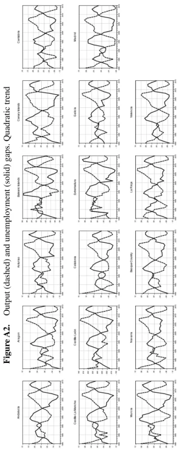
(9) Regional differences in the Okun’s Relationship: New Evidence for Spain (1980-2015) 145. mer than in the latter. This result suggests that there might be important differences among the whole group of Spanish regions. Precisely, the articles by Villaverde and Maza (2007, 2009) test that hypothesis. They estimate the Okun’s relationship (the gap model) and conclude that there are quite important differences. These authors also point out that those differences are a consequence of the different growth rates in labor productivity among the Spanish regions. The work by Clar-López et al. (2014) is particularly focused on forecasting. Their goal is to assess the relative precision of forecasting models based on the Okun’s law in comparison to alternative methods. They draw the conclusion that, in general terms and in most regions, the Okun’s law models enhance the forecasting power, although the accuracy of the models is not good enough to provide reliable predictions. Finally, Melguizo (2017) makes use of a higher territorial disaggregation and takes the Spanish provinces (NUTS-3 breakdown) as the observational unit. The main conclusion is that the variability found at the provincial level in the Okun’s law relationship is a relevant issue that might deserve additional attention in the future research agenda.. 4. 4.1.. Data and econometric results Database. In this section we summarize the empirical results for the estimation of the Okun’s relationship in the 17 Spanish regions. Following the discussion in Adanu (2005) and Villaverde and Maza (2009) the first step of the analysis is to obtain an estimate of the output and unemployment gaps. To this end, we use the BD-MORES dataset, provided by the Ministry of Finance, which is a regional dataset providing regional accounting type data on output and its components. The BD-MORES provides data for the period 1980-2008, and therefore precludes any analysis after the onset of the Great Recession. To perform such analysis, the growth rates of GDP (provided by the official Regional Accounts Contabilidad Regional de España, elaborated by the Spanish Statistical Office INE) and the BD-MORES dataset have been combined. Specifically, we have calculated the growth rate of regional gross value added for each year from 2008 to 2015, and applied these growth rates to the existing BDMORES data on 2008. Thus, the BD-MORES data has been projected to more recent periods, which allows to take into account the effect of the recession in the Okun’s relationship at the regional level. The unemployment data is taken from the Labour Force Survey, developed by the Spanish Statistical Office (INE). Specifically, we use the regional unemployment rate for the period 1980-2015. Given that the BD-MORES data is in annual frequency, the annual average regional unemployment rate has been computed. In order to obtain estimates for the output and unemployment gaps we use the Hodrick-Prescott filter (HP) and the Quadratic Trend (QT) approach. In the first case the HP filter has been applied to the level output and unemployment rate series, using a value for λ of 100, as suggested by most of the literature for annual data. The resultInvestigaciones Regionales – Journal of Regional Research, 41 (2018) – Páginas 137 a 165.
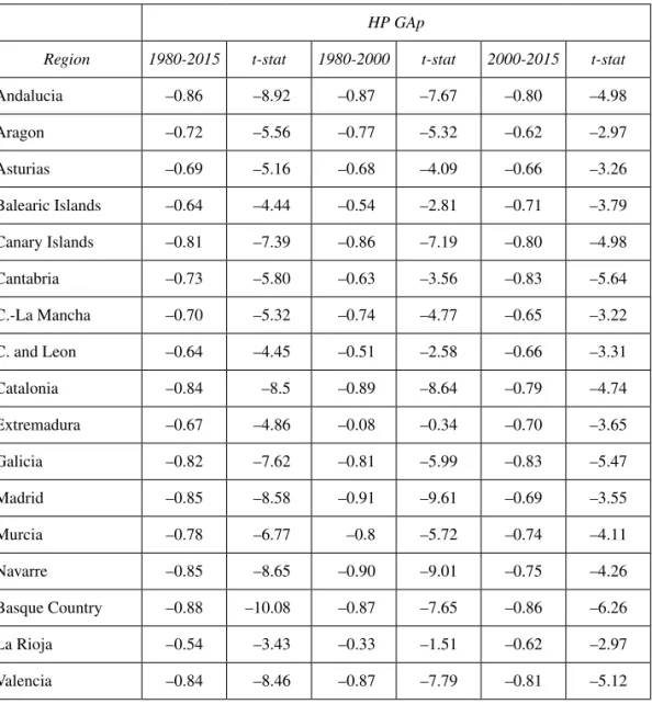
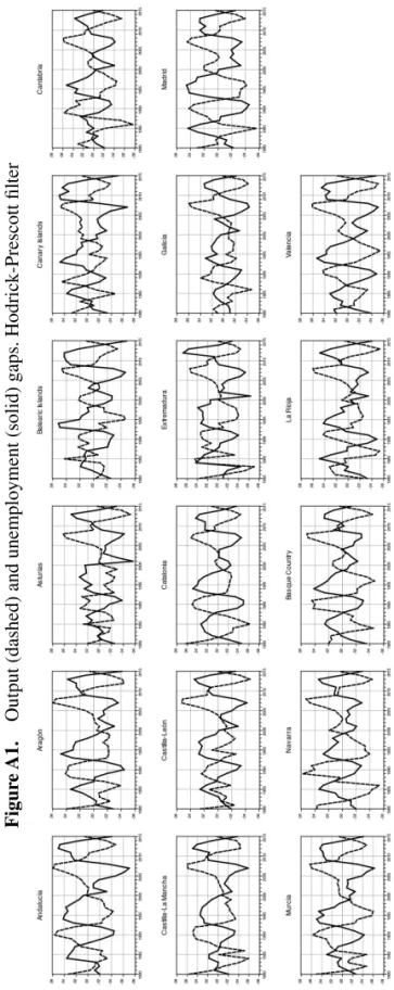
(10) 146. Bande, R., Martín-Román, Á.. ing detrended series are regarded as the cyclical component of output and unemployment, and are afterwards used in the estimations. As regards the QT procedure, each series was regressed on a quadratic trend and the resulting residuals were interpreted as the measure of the cyclical components. Figures A1 and A2 in the appendix depict these cyclical components, and unveil a clear negative relationship between output and unemployment gaps, even though with notorious regional differences in the intensity of such relationship. Moreover, it is clear that different lag structures across regions must be taken into account in the subsequent empirical work. Interestingly, the relationship seems to be strongest among the more industrialised regions, e. g., Madrid or Catalonia, whereas the link in less developed regions, as Castile and Leon or Asturias, seems to be weaker. A similar pattern was found by Adanu (2005) for the Canadian regions. Notwithstanding, the intensity of the negative relationship seems to be stronger when we use the QT rather than the Hodrick-Prescott cycles. Additionally, the Okun’s trade-off seems to have vanished through time in some regions, while being reinforced in others. The negative correlation seems to be strongest in the 80’s in Madrid, regions along the Ebro Axis (Navarre, La Rioja and Aragón) and Catalonia, whereas is extremely low in more rural regions, as Extremadura or La Rioja. During the first years of the current century the correlation coefficient has tended to increase in those regions where it was low in the 80’s, and to be reduced in the regions where it used to be relatively high. Table A1 in the appendix summarises these correlation coefficients for the whole sample and for two subsamples, namely 1980 to 2000 and 2000 to 2015. Note that all of these correlation coefficients are significant, as indicated by the corresponding t-statistics. This result is a reflection of the regional heterogeneity in the relationship between output and unemployment cycles, and reinforces the motivation of this article. 4.2. Baseline model. The empirical counterpart of the theoretical model discussed in section 2 establishes a stable relationship between the output gap and the unemployment gap, of the type: p. ygapt = a + bugapt + / cj ygapt - j + ft. (5). j=1. where ygapt is the log of the output gap, ugapt is the unemployment rate gap and εt is an error term. We allow for a lag structure in this equation, in order to capture adequately the dynamics of the relationship between output and unemployment gaps. As discussed below, the optimal lag structure will be determined following standard statistical information criteria. Given these estimates of output and unemployment gaps, the next step is to ensure that these series are stationary, or if not, whether they are cointegrated, otherwise the estimation of equation (5) could provide flawed results due to a Investigaciones Regionales – Journal of Regional Research, 41 (2018) – Páginas 137 a 165.
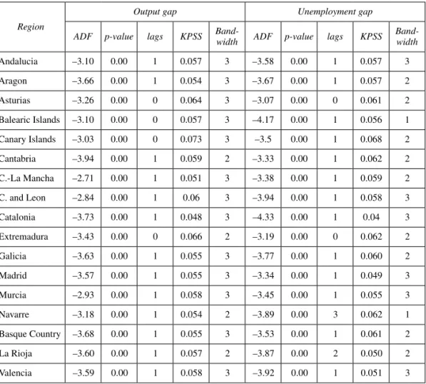
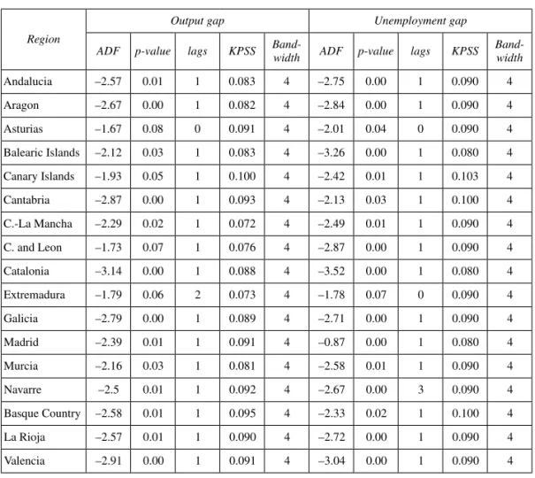
(11) Regional differences in the Okun’s Relationship: New Evidence for Spain (1980-2015) 147. spurious relationship between the involved variables. Therefore, standard unit root tests for each of the output and unemployment gaps were computed. Results, summarised in tables 1 and 2, suggest that all of the estimated gaps are stationary in levels, i. e., they do not exhibit a unit root. p-values of the ADF tests are well below 5%, whereas for the KPSS test all of the estimated test statistics are below the corresponding 5% critical value, which is approximately 0.46. Therefore, results are robust to the type of test (ADF and KPSS tests are reported) and to the test specification 5. Table 1. Unit root tests. Hodrick-Prescott filter gaps Output gap Region. Unemployment gap. ADF. p-value. lags. KPSS. Bandwidth. ADF. p-value. lags. KPSS. Bandwidth. Andalucia. –3.10. 0.00. 1. 0.057. 3. –3.58. 0.00. 1. 0.057. 3. Aragon. –3.66. 0.00. 1. 0.054. 3. –3.67. 0.00. 1. 0.057. 2. Asturias. –3.26. 0.00. 0. 0.064. 3. –3.07. 0.00. 0. 0.061. 2. Balearic Islands. –3.10. 0.00. 0. 0.057. 3. –4.17. 0.00. 1. 0.056. 1. Canary Islands. –3.03. 0.00. 0. 0.073. 3. –3.5. 0.00. 1. 0.068. 2. Cantabria. –3.94. 0.00. 1. 0.059. 2. –3.33. 0.00. 1. 0.062. 2. C.-La Mancha. –2.71. 0.00. 1. 0.051. 3. –3.38. 0.00. 1. 0.059. 2. C. and Leon. –2.84. 0.00. 1. 0.06. 3. –3.94. 0.00. 1. 0.058. 3. Catalonia. –3.73. 0.00. 1. 0.048. 3. –4.33. 0.00. 1. 0.04. 3. Extremadura. –3.43. 0.00. 0. 0.066. 2. –3.19. 0.00. 0. 0.062. 2. Galicia. –3.63. 0.00. 1. 0.055. 3. –3.77. 0.00. 1. 0.060. 2. Madrid. –3.57. 0.00. 1. 0.055. 3. –3.34. 0.00. 1. 0.049. 3. Murcia. –2.93. 0.00. 1. 0.058. 3. –3.45. 0.00. 1. 0.055. 3. Navarre. –3.18. 0.00. 1. 0.054. 2. –3.89. 0.00. 3. 0.062. 1. Basque Country. –3.68. 0.00. 1. 0.055. 3. –3.53. 0.00. 1. 0.061. 2. La Rioja. –3.60. 0.00. 1. 0.057. 2. –3.87. 0.00. 2. 0.050. 2. Valencia. –3.59. 0.00. 1. 0.058. 3. –3.92. 0.00. 1. 0.051. 3. Notes: ADF is the Augmented Dickey Fuller test-statistic, while KPSS is the Kwiatkowski-Phillips-Schmidt-Shin test. The 5% level critical value for the KPSS test is approximately 0.46. 5 Given the characteristics of the time series depicted in figures A1 and A2 in the appendix, it becomes clear that none of the gap series show a trend or a constant, i. e., they evolve stationary around a zero-mean. Nevertheless, we also computed the ADF and the KPSS test under the null of a linear trend. Results, obviously, reject non-stationarity of the series. These auxiliary tests are not reported for brevity but are available from the authors upon request.. Investigaciones Regionales – Journal of Regional Research, 41 (2018) – Páginas 137 a 165.
(12) 148. Bande, R., Martín-Román, Á.. Table 2. Unit root tests. Quadratic trends gaps Output gap Region. Unemployment gap. ADF. p-value. lags. KPSS. Bandwidth. ADF. p-value. lags. KPSS. Bandwidth. Andalucia. –2.57. 0.01. 1. 0.083. 4. –2.75. 0.00. 1. 0.090. 4. Aragon. –2.67. 0.00. 1. 0.082. 4. –2.84. 0.00. 1. 0.090. 4. Asturias. –1.67. 0.08. 0. 0.091. 4. –2.01. 0.04. 0. 0.090. 4. Balearic Islands. –2.12. 0.03. 1. 0.083. 4. –3.26. 0.00. 1. 0.080. 4. Canary Islands. –1.93. 0.05. 1. 0.100. 4. –2.42. 0.01. 1. 0.103. 4. Cantabria. –2.87. 0.00. 1. 0.093. 4. –2.13. 0.03. 1. 0.100. 4. C.-La Mancha. –2.29. 0.02. 1. 0.072. 4. –2.49. 0.01. 1. 0.090. 4. C. and Leon. –1.73. 0.07. 1. 0.076. 4. –2.87. 0.00. 1. 0.090. 4. Catalonia. –3.14. 0.00. 1. 0.088. 4. –3.52. 0.00. 1. 0.080. 4. Extremadura. –1.79. 0.06. 2. 0.073. 4. –1.78. 0.07. 0. 0.090. 4. Galicia. –2.79. 0.00. 1. 0.089. 4. –2.71. 0.00. 1. 0.090. 4. Madrid. –2.39. 0.01. 1. 0.091. 4. –0.87. 0.00. 1. 0.080. 4. Murcia. –2.16. 0.03. 1. 0.081. 4. –2.58. 0.01. 1. 0.090. 4. Navarre. –2.5. 0.01. 1. 0.092. 4. –2.67. 0.00. 3. 0.090. 4. Basque Country. –2.58. 0.01. 1. 0.095. 4. –2.33. 0.02. 1. 0.100. 4. La Rioja. –2.57. 0.01. 1. 0.090. 4. –2.72. 0.00. 1. 0.090. 4. Valencia. –2.91. 0.00. 1. 0.091. 4. –3.04. 0.00. 1. 0.090. 4. Notes: ADF is the Augmented Dickey Fuller test-statistic, while KPSS is the Kwiatkowski-Phillips-Schmidt-Shin test. The 5% level critical value for the KPSS test is approximately 0.46.. Once that the dynamic properties of the time series involved in the estimations have been identified, the next step is to estimate the model in equation (5). The empirical strategy consists in estimating equation (5) for each region in the sample period 1980-2015, allowing for different lag structures, i. e., each regional equation will include an optimal number of lags. This strategy is the same as in Adanu (2005), but contrary to Villaverde and Maza (2009), who impose a similar dynamic structure to their regional equations. The optimal number of lags has been selected using the standard statistical information criteria, i. e., the Akaike and the Schwarz criteria. Each model was estimated, using both versions of the gaps, including up to 5 lags in each equation, selecting the lag structure that maximized the criteria. In general, both criteria suggest a similar lag structure for each equation. The coefficient on the unemployment gap provides the Okun’s coefficient, i. e., the output gap variation after an unemployment gap variation. We expect this coefficient to be negative, while the wide divergence of results Investigaciones Regionales – Journal of Regional Research, 41 (2018) – Páginas 137 a 165.
(13) Regional differences in the Okun’s Relationship: New Evidence for Spain (1980-2015) 149. in the existing literature precludes any prior as regards the value that should exhibit. Nevertheless, the Okun’s coefficient can be interpreted as the short run elasticity of the output gap with respect to the unemployment gap. We also report the long run solution of each model, which provides the long run impact of a unit change in the unemployment gap on the output gap, i. e.,. the long run Okun’s coefficient. More formally, if we compute the long run solution of equation (5) under the assumption that variables stabilise around a long run value (denoted by subscript LR), we may write: p. ygapLR = a + bugapLR + / cj ygapLR. (6). f 1 - / cj p ygapLR = a + bugapLR. (7). j=1. and therefore: p. j=1. so the long run value of ygap may be written as: ygapLR =. b a + ugapLR 1 - / j cj 1 - / j cj. (8). or ygapLR = z0 + z1 ugapLR. (9). b a , and z1 = is the long run elasticity of the output 1 - / j cj 1 - / j cj gap with respect to to the unemployment gap. This elasticity measures the long run impact of a change in the unemployment gap on the former, once that the dynamics of adjustment have settled down. Note that the short run elasticity b can be greater than φ (in which case it overshoots its long run value) or lower, in which case it converges gradually towards the long run equilibrium. Karanassou et al. (2010) provide a good summary of the differences between short run, long run and steady state solutions of dynamic models.. where z0 =. Equation (5) is therefore estimated by OLS for each of the 17 Spanish regions using the dataset described above. The sample period is 1980-2015, and a number of misspecification tests have been conducted after estimation to ensure a proper setup of the model. Results are summarised in Table 3 for the HP gap and in Table 4 for the QT version of the gap.. Investigaciones Regionales – Journal of Regional Research, 41 (2018) – Páginas 137 a 165.
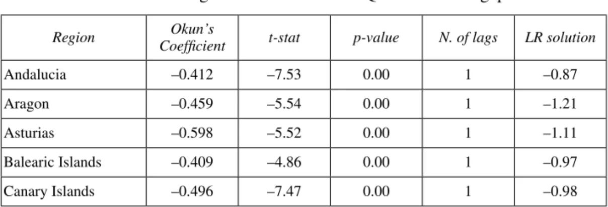
(14) 150. Bande, R., Martín-Román, Á.. Table 3. Regional OLS estimates. HP gap Okun’s Coefficient. t-stat. p-value. N. of lags. LR solution. Andalucia. –0.504. –6.40. 0.00. 1. –0.87. Aragon. –0.524. –4.60. 0.00. 1. –1.00. Asturias. –0.562. –4.12. 0.00. 1. –0.80. Balearic Islands. –0.425. –4.33. 0.00. 1. –0.72. Canary Islands. –0.522. –6.34. 0.00. 1. –0.73. Cantabria. –0.524. –3.07. 0.00. 2. –0.83. C.-La Mancha. –0.652. –4.50. 0.00. 2. –1.35. C. and Leon. –0.457. –3.55. 0.00. 1. –0.84. Catalonia. –0.607. –7.75. 0.00. 1. –0.98. Extremadura. –0.399. –2.71. 0.00. 4. –0.59. Galicia. –0.729. –6.49. 0.00. 1. –1.18. Madrid. –0.528. –4.7. 0.00. 2. –0.70. Murcia. –0.614. –5.95. 0.00. 1. –1.10. Navarre. –1.069. –6.04. 0.00. 1. –1.51. Basque Country. –0.955. –7.19. 0.00. 1. –1.31. La Rioja. –0.555. –5.11. 0.00. 1. –1.52. Valencia. –0.617. –12.14. 0.00. 1. –1.20. Spain. –0.495. –15.28. 0.00. 5. –0.79. Region. Notes: OLS estimates of the regional models. Fourth column indicates the optimal lag length suggested by the AIC and the SBC.. Table 4. Regional OLS estimates. Quadratic trend gap Okun’s Coefficient. t-stat. p-value. N. of lags. LR solution. Andalucia. –0.412. –7.53. 0.00. 1. –0.87. Aragon. –0.459. –5.54. 0.00. 1. –1.21. Asturias. –0.598. –5.52. 0.00. 1. –1.11. Balearic Islands. –0.409. –4.86. 0.00. 1. –0.97. Canary Islands. –0.496. –7.47. 0.00. 1. –0.98. Region. Investigaciones Regionales – Journal of Regional Research, 41 (2018) – Páginas 137 a 165.
(15) Regional differences in the Okun’s Relationship: New Evidence for Spain (1980-2015) 151. Table 4. (cont.) Okun’s Coefficient. t-stat. p-value. N. of lags. LR solution. Cantabria. –0.538. –3.96. 0.00. 2. –1.06. C.-La Mancha. –0.466. –5.67. 0.00. 1. –1.06. C. and Leon. –0.439. –5.75. 0.00. 1. –1.10. Catalonia. –0.565. –8.00. 0.00. 1. –1.16. Extremadura. –0.318. –8.86. 0.00. 4. –0.83. Galicia. –0.601. –4.70. 0.00. 1. –1.09. Madrid. –0.616. –5.81. 0.00. 2. –1.10. Murcia. –0.457. –5.11. 0.00. 1. –1.18. Navarre. –0.894. –7.36. 0.00. 1. –1.81. Basque Country. –0.758. –6.38. 0.00. 1. –1.25. La Rioja. –0.561. –8.09. 0.00. 1. –1.75. Valencia. –0.603. –6.36. 0.00. 1. –1.22. Spain. –0.425. –17.49. 0.00. 5. –0.97. Region. Notes: OLS estimates of the regional models. Fourth column indicates the optimal lag length suggested by the AIC and the SBC.. In both tables it can be observed that all estimated coefficients are significant and show the expected negative sign. Also, there is a wide range of values for the optimal lag structure. The last row in each table provides the coefficient obtained for the whole Spanish economy, estimated by pooling all of the regional observations and including a regional fixed effect. The general picture that emerges from Tables 3 and 4 is that the degree of variation in the relationship between output and unemployment gaps is quite large. This implies that the use of regional data will be helpful in identifying the magnitude of the relationship. The estimated coefficients at the aggregate level are –0.495 and –0.425 for the HP and the QT gaps respectively. However, these coefficients hide enormous regional disparities. For instance, as regards the HP gap, the northern regions of Navarre and the Basque Country show the largest coefficients of –1.06 and –0.955 respectively, i. e. more than twice the national average. Regions as Galicia or Valencia show also relatively high coefficients (–0.729 and –0.617). At the same time, other regions show lower coefficients as, e. g., the Balearic Islands (–0.425) or Extremadura (–0.399). This variation in the short run coefficients is somewhat translated to the long run coefficients, i. e., once that dynamics are settled down. Thus, 5 out of 17 regions show a coefficient greater than 1 in absolute value (La Rioja, –1.52; Navarre, –1.51; Basque Country, –1.31; Castilla-La Mancha, –1.35 and Galicia, –1.18). On the other side of the spectrum there are a number of regions exhibiting lower values, as Madrid (–0.70), the Baleric Islands (–0.72) or Extremadura (–0.59). Investigaciones Regionales – Journal of Regional Research, 41 (2018) – Páginas 137 a 165.
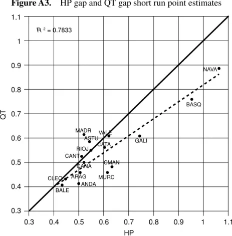
(16) 152. Bande, R., Martín-Román, Á.. When the QT gap is considered a similar conclusion holds 6. As regards short run coefficients, again the northern regions of Basque Country and Navarre show the highest values (–0.758 and –0.894, respectively,), while the Balearic Islands and Extremadura remain as the regions with the lowest values (–0.409 and –0.317 respectively). Nevertheless, the estimated slope coefficients are in general lower for the QT specification than those in the HP gap version. Once that the short run dynamics have been allowed to settle down and the long run coefficient is computed, wit is found that La Rioja and Navarre have the greatest elasticities (–1.75 and –1.81 respectively), while the southern regions of Andalucía and Extremadura have the lowest values for such coefficient (–0.87 and –0.83). Thus, in spite of differences in the magnitudes of the estimated coefficients, the image that emerges from these results is that there is a large degree of heterogeneity in the regional response of output to the unemployment gap.. 4.3.. Extensions. We next explore further this relationship between the output and the unemployment gap by performing two additional exercises. First, we investigate whether the Okun’s law can be estimated separately for different groups of regions, since previous literature has shown that different groups or clusters of regions can be considered when analysing the labour market outcomes (see inter alia Bande et al., 2008, Bande and Karanassou, 2009, 2014, Bande et al., 2012, or Sala and Trivin, 2014). Secondly, given that the sample covers a period of time before and after the Great Recession, it is explored whether there is a cyclical asymmetry in the response of the output gap to the unemployment gap 7. In order to perform such analysis, two different samples will be used, one from 2001 to 2008 and another one from 2009 to 2015, pooling the regional data to exploit the cross-sectional dimension. We first start by grouping Spanish regions depending on the value of the short run Okun’s coefficient. Using the HP gap model, the median of the regional distribution of estimated Okun’s coefficients was computed, and Spanish regions were classified into two broad groups: first, those regions with an estimated individual slope coefficient greater than the median value (so called «High group») and those with a lower value (so called «Low group»). While it is obvious that a greater coefficient should be expected for the former group than for the latter, this exercise allows an even more precise identification of the Okun’s relationship through the use of panel data. Pooling data into these two broad groups increases significantly the number of available observations, and thus provides a more robust estimate of both the short run and long run coefficients. Table 5 summarises the classification exercise. Note that not 6 However, point estimates of coefficients show in general lower values tan those obtained for the HP gap. In Figure A3 in the appendix HP gap versus QT gap short run estimates are depicted. 7 A large branch of the existing literature has shown that the Okun relationship is highly asymmetric along the business cycle.. Investigaciones Regionales – Journal of Regional Research, 41 (2018) – Páginas 137 a 165.
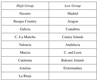
(17) Regional differences in the Okun’s Relationship: New Evidence for Spain (1980-2015) 153. necessarily those regions allocated to the High (Low) group correspond with regions where the unemployment rate is low (high). Differences in the Okun coefficient may be interpreted along the lines of the theoretical model presented in Section 2 in terms of different production functions, which result in heterogeneous regional output response to labour market shocks. Table 5. Classification of Spanish regions High Group. Low Group. Navarre. Madrid. Basque Country. Aragon. Galicia. Cantabria. C.-La Mancha. Canary Islands. Valencia. Andalucia. Murcia. C. and Leon. Catalonia. Balearic Islands. Asturias. Extremadura. La Rioja Median: –0.555.. After clustering the 17 Spanish regions into these groups, the observations for each group were pooled, and the Okun’s coefficient was estimated using a fixed effects panel model. In this model, and following the same methodology outlined above, specific dynamics for the output gap were allowed, selecting the optimal number of lags on the basis of the AIC and the SBC criteria. The fixed effects estimator is consistent in dynamic panels with constant slopes as the number of time periods T " 3 for a fixed number of cross sections N. However, the literature (see for instance Baltagi, 2013) has shown that when T is small relative to N, the OLS estimator is inconsistent. For instance, when N " 3 for a fixed T the Nickell bias will be present, and thus the true value of the coefficient on the lagged dependent variable would be underestimated. In this case, the standard approach is to use a General Method of Moments (GMM) estimator, which first differences the data to remove the fixed effects, and then applies an instrumental variables estimator, using further lags of the endogenous as instruments for the lagged dependent. The DPD estimator by Arellano and Bond (1991) or the Blundell and Bond (1998) estimator are straightforward options. We have computed both the OLS and GMM estimator (using the Arellano and Bond DPD), using further lags of the endogenous variable as instruments. In any case, we do not expect the Nickell bias to be severe, since the Investigaciones Regionales – Journal of Regional Research, 41 (2018) – Páginas 137 a 165.
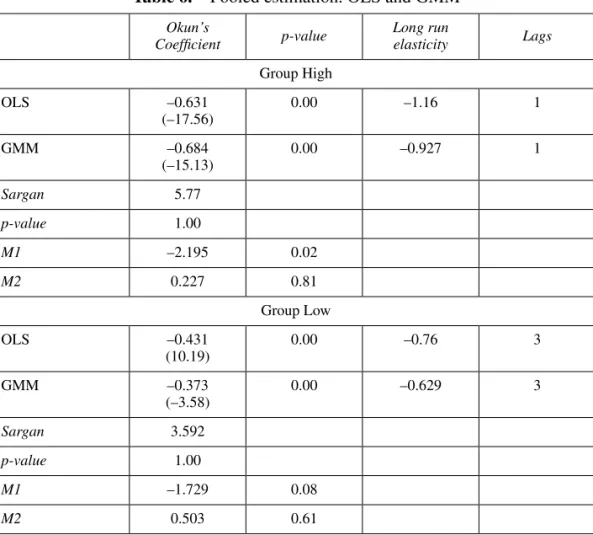
(18) 154. Bande, R., Martín-Román, Á.. number of cross section in each group is smaller than the number of time observations. Our results in Table 6 suggest indeed that this is the case, with similar estimates for both specifications 8. Table 6. Pooled estimation. OLS and GMM Okun’s Coefficient. p-value. Long run elasticity. Lags. Group High OLS. –0.631 (–17.56). 0.00. –1.16. 1. GMM. –0.684 (–15.13). 0.00. –0.927. 1. Sargan. 5.77. p-value. 1.00. M1. –2.195. 0.02. M2. 0.227. 0.81 Group Low. OLS. –0.431 (10.19). 0.00. –0.76. 3. GMM. –0.373 (–3.58). 0.00. –0.629. 3. Sargan. 3.592. p-value. 1.00. M1. –1.729. 0.08. M2. 0.503. 0.61. Notes: Fixed effects OLS and Arellano-Bond GMM estimator, t-statistics in parentheses.. Results in Table 6 suggest that there exist significant differences between both groups as regards the magnitude of the Okun’s relationship. The point estimate for the coefficient of the High group is –0.631, 200 basic points greater than the estimate for the Low group (–0.431). Further, these differences do not vanish when the 8 For brevity, Table 6 reports only estimated Okun’s coefficients and the corresponding long run solutions of the model. Full results, with the estimated coefficients for the lagged endogenous are available from the authors upon request. Also, note that the value of the Sargan test as well as those of the Arellano and Bond M1 and M2 point to the validity of our instruments choice. Thus, the p-value of the Sargan tests does not allow rejection of the null hypothesis that the over-identifying restrictions are valid. Also, the M1 and M2 statistics indicate that residuals show first-order, but not second order autocorrelation. Results with other GMM estimators are similar to those shown in the table, but are not reported for brevity.. Investigaciones Regionales – Journal of Regional Research, 41 (2018) – Páginas 137 a 165.
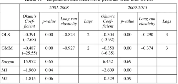
(19) Regional differences in the Okun’s Relationship: New Evidence for Spain (1980-2015) 155. model is estimated with the Arellano and Bond GMM estimator, since the reported coefficients are similar to those of the OLS estimation. Additionally, when the long run solution of the model for each group are computed, the differences become even more apparent, with long run elasticities of –1.16 and –0.76 for the OLS version, and –0.927 and –0.629 for the GMM estimation. Therefore, the analysis confirms the existence of strong differences in the relationship between output and unemployment gaps between both groups of Spanish regions. We next turn our attention to the analysis of potential asymmetries during the business cycle. In this case, we first use all of the regional data to estimate separate models for the sub-periods 2001-2008 and 2009-2015 9. If there is cyclical asymmetry, we should find significant different Okun’s coefficients for each sub-sample 10. Table 7 summarises both the OLS and GMM estimations. Given that for both subsamples the number of cross-sections is clearly larger than the number of time periods, it is likely that OLS estimates are biased, as explained above. Thus, in this case we give more credit to the GMM estimates, which is reinforced after inspection of the Sargan test of overidentifying restrictions and the Arellano-Bond M1 and M2 autocorrelation tests. Results in Table 7 uncover the existence of significant and strong differences in the Okun’s relationship along the business cycle. In the booming period of 2001-2008, the Okun’s coefficient was of –0.487, with a long run coefficient of –0.927, i. e., for each percentage point of unemployment above (below) its trend, GDP growth was almost a half percentage point below (above) its trend. When the recession kicked in, however, this trade-off was significantly reduced, since the short run coefficient falls to –0.350, with a long run elasticity of –0.374, almost 40% of the estimated effect for the booming period. In other words, there exists a clear asymmetry in the Okun’s relationship in booming and recession phases of the Spanish business cycle. It should be pointed out, however, that the important regulatory changes in the Spanish labour market, as a consequence of the labour reform of 2012, could be affecting the results obtained for the period 2009-2015, at least to some degree. In this vein, Jimeno and Santos (2014) establish that labour market institutions are key to understand employment (and obviously unemployment) dynamics in Spain, particularly in the context 9 The choice of these sub-periods is based on the available data for the recession period. Since available data for the recession and post-recession period at the moment of writing was 2009-2015, we decided to use a similar number of periods prior to the onset of the recession, which additionally coincide with one of the strongest booms of the Spanish economy in the last decades. Therefore, estimates in Table 7 provide information for two extremely divergent moments of the recent Spanish business cycle: one in which GDP growth was one of the strongest in the European Union, and another one in which Spain led the international indicators as regards job destruction and unemployment growth. 10 The empirical finding of different Okun’s coefficients in these two subperiods would be an indication that our initial estimates in Tables 4 and 5 suffered from structural instability. Actually, the Chow test for structural break in 2008 or 2009 was performed for the estimates in those tables, but results persistently did not allow to reject the null of no structural break. This, however, may be due to the small sample size after the assumed structural break as compared to the pre-recession sample. Other structural stability indicators, as recursive least squares (CUSUM and CUSUMQ) suggested some signs of structural break in our estimations. Results in Table 7 confirm this hypothesis.. Investigaciones Regionales – Journal of Regional Research, 41 (2018) – Páginas 137 a 165.
(20) 156. Bande, R., Martín-Román, Á.. of the Great Recession. Even more specifically, there are some works showing that labour reforms having an effect on EPL are likely to modify the Okun’s betas (e. g. Boeri, 2011). The main goal of this article is not, however, to measure accurately to what extent the labour reform of 2012 has altered the Okun’s coefficient at the regional level. That would be an appealing topic for future research. Table 7. Expansion and Recession periods. OLS and GMM 2001-2008 Okum’s Coefficient. 2009-2015. p-value. Long run elasticity. Lags. Okum’s Coefficient. p-value. Long run elasticity. Lags. OLS. –0.391 (–7.68). 0.00. –0.823. 2. –0.304 (–3.92). 0.00. –0.290. 3. GMM. –0.487 (–25.55). 0.00. –0.927. 2. –0.350 (–6.35). 0.00. –0.374. 3. Sargan. 15.972. 0.65. 6.452. 0.69. M1. –1.960. 0.04. –2.609. 0.00. M2. –1.815. 0.06. –0.529. 0.59. Notes: Fixed effects OLS and Arellano-Bond GMM estimator, t-statistics in parentheses. Sargan refers to the Sargan test of overidentifying restrictions. M1 and M2 are the Arellano-Bond first and second order autocorrelation tests.. 5.. Conclusions. In this article we estimate the Okun’s law for the Spanish regions, providing new empirical evidence on the relationship between the unemployment rate and the output growth at the regional level. Following the approach developed by Adanu (2005) and applyng it for the Spanish regions, we depart from Villaverde and Maza (2009) and Clar-López et al. (2014), the two more relevant published articles addressing the Okun’s law for the Spanish regions, in several forms. In order to be more precise, the «gap version» with the output growth on the left-hand side of the equation is our benchmark model. As mentioned before, the gap model links the difference between actual and natural unemployment with the difference between the log of actual output and the log of potential output. However, several modifications in this baseline model have been carried out, which may be considered also novelties of this work. First, a lag structure in the Okun’s equation has been allowed for, in order to capture adequately the dynamics of the relationship between output and unemployment gaps. This, in turn, allows to estimate both the short run and the long run elasticities for the Okun’s law. Second, two different measures of the unemployment and output gaps were considered, based on the HP filter and the QT procedure, respectively, in order to provide robustness to our analysis. Third, after the time series study, Spanish regions have been pooled into two groups Investigaciones Regionales – Journal of Regional Research, 41 (2018) – Páginas 137 a 165.
(21) Regional differences in the Okun’s Relationship: New Evidence for Spain (1980-2015) 157. and perform a panel data approach. OLS and GMM estimates with panel data methodology are obtained and compared. Finally, we also take into account the potential asymmetries throughout the business cycle and estimate distinct elasticities for the boom period ranging from 2000 to 2008 and the recessionary period comprised between 2009 and 2015. As for the results, after checking that our series are stationary, we find that all coefficients are significant and show the expected negative sign. Thus, in all the Spanish regions the Okun’s law seems to portray the cyclical behaviour of local labour markets to a greater or lesser extent. However, there is a wide variability in the point estimates across regions, both for the short run and the long run output-unemployment elasticities. Moreover, these outcomes are robust to the different gap specifications, i. e. HP filter or QT procedure. As an example of that, and regarding the short run coefficients estimated by means of the HP filter, our findings show that the northern regions of Navarre and the Basque Country exhibit the largest coefficients: –1.06 and –0.955 respectively. On the other hand, the Balearic Islands (–0.425) and Extremadura (–0.399) show the lowest coefficients. These huge disparities imply that the use of regional data will be helpful in identifying the magnitude of the relationship, particularly if the Okun’s law is used as a rule of thumb for regional economic policy purposes. Two different extensions from our benchmark approach have been carried out. First, we pool the Spanish regions so as to obtain a single database with both time and cross-regional variability, which allows to make use of panel data techniques. The models were subsequently estimated by OLS and GMM, and results were compared. Spanish regions were broken down into two blocks, according to the value of the short run Okun’s coefficient. We find that there are significant differences between the «high» and «low» elasticity groups and that the OLS and GMM estimates show a similar pattern. This outcome reinforces the idea of the significance of regional analysis in order to recommend more accurate economic policy prescriptions with regard to the business cycle. In the second exercise, it was tested whether there are cyclical asymmetries in the Okun’s coefficients. With this aim, and making use of all the regional data to estimate separate models for the sub-periods 2001-2008 and 2009-2015, it is found that the Okun’s cyclical elasticity is significantly higher (in absolute terms) in the expansionary period of 2000-2008 than in the recessionary period of 2009-2015. Put in other words, a marked asymmetry in the Okun’s relationship during booms and downturns is detected.. References Abowd, J. M., and Kramarz, F. (2003): «The costs of hiring and separations», Labour Economics, 10(5), 499-530. Adanu, K. (2005): «A cross-province comparison of Okun’s coefficient for Canada», Applied Economics, 37(5), 561-570. Apergis, N., and Rezitis, A. (2003): «An examination of Okun’s law: evidence from regional areas in Greece», Applied Economics, 35(10), 1147-1151. Investigaciones Regionales – Journal of Regional Research, 41 (2018) – Páginas 137 a 165.
(22) 158. Bande, R., Martín-Román, Á.. Arellano, M., and Bond, S. (1991): «Some tests of specification for panel data: Monte Carlo evidence and an application to employment equations», The Review of Economic Studies, 58(2), 277-297. Balakrishnan, R., Das, M., and Kannan, P. (2010): «Unemployment dynamics during recessions and recoveries: Okun’s law and beyond», IMF World Economic Outlook, 69108. Ball, L. M., Leigh, D., and Loungani, P. (2013): «Okun’s Law: Fit at Fifty?», NBER Working Paper Series, 18668. Bande, R., Fernández, M., and Montuenga, V. (2008): «Regional Unemployment in Spain: Disparities, Business Cycle and Wage Setting», Labour Economics, 15(5), 885-914. — (2012): «Wage Flexibility and Local Labour Markets: Homogeneity of the Wage Curve in Spain», Investigaciones Regionales, 24, 173-196. Bande, R., and Karanassou, M. (2009): «Labour Market Flexibility and Regional Unemploymeny Rate Dynamics: Spain 1980-1995», Papers in Regional Science, 88(1), 181-207. — (2014): «Spanish Regional Unemployment revisited: The Role of Capital Accummulation», Regional Studies, 48(11), 1863-1883. Binet, M. E., and Facchini, F. (2013): «Okun’s law in the French regions: a cross-regional comparison», Economics Bulletin, 33(1), 420-433. Blanchard, O. (1997): Macroeconomics, Prentice Hall, Upper Saddle River, NJ, 384-387. Blundell, R., and Bond, S. (1998): «Initial conditions and moment restrictions in dynamic panel data models», Journal of Econometrics, 87(1), 115-143. Boeri, T. (2011): «Institutional reforms and dualism in European labor markets», Handbook of labor economics, 4 (Part B), 1173-1236. Cazes, S., Verick, S., and Al Hussami, F. (2013): «Why did unemployment respond so differently to the global financial crisis across countries? Insights from Okun’s Law», IZA Journal of Labor Policy, 2(1), 1-18. Christopoulos, D. K. (2004): «The relationship between output and unemployment: Evidence from Greek regions», Papers in Regional Science, 83(3), 611-620. Clar-Lopez, M., López-Tamayo, J., and Ramos, R. (2014): «Unemployment forecasts, time varying coefficient models and the Okun’s law in Spanish regions», Economics and Business Letters, 3(4), 247-262. Crespo-Cuaresma, J. (2003): «Okun’s law revisited», Oxford Bulletin of Economics and Statistics, 65(4), 439-451. Daly, M., Fernald, J., Jordà, Ò., and Nechio, F. (2014): «Interpreting deviations from Okun’s Law», FRBSF Economic Letter, 12. Daly, M., and Hobijn, B. (2010): «Okun’s Law and the Unemployment Surprise of 2009», FRBSF Economic Letter, 7. Durech, R., Minea, A., Mustea, L., and Slusna, L. (2014): «Regional evidence on Okun’s law in Czech Republic and Slovakia», Economic Modelling, 42, 57-65. Freeman, D. G. (2000): «Regional tests of Okun’s law», International Advances in Economic Research, 6(3), 557-570. Gordon, R. J. (1984): «Unemployment and potential output in the 1980s», Brookings Papers on Economic Activity, 2, 537-568. Goux, D., Maurin, E., and Pauchet, M. (2001): «Fixed-term contracts and the dynamics of labour demand», European Economic Review, 45(3), 533-552. Guisinger, A. Y., Hernandez-Murillo, R., Owyang, M., and Sinclair, T. M. (2015): «A StateLevel Analysis of Okun’s Law. Research Division, Federal Reserve Bank of St. Louis», Working Paper Series, 2015-029A. Hamermesh, D. S. (1996): Labor demand, Princeton University Press. Hamermesh, D. S., and Pfann, G. A. (1996): «Adjustment costs in factor demand», Journal of Economic Literature, 34(3), 1264-1292. Investigaciones Regionales – Journal of Regional Research, 41 (2018) – Páginas 137 a 165.
(23) Regional differences in the Okun’s Relationship: New Evidence for Spain (1980-2015) 159. Harris, R., and Silverstone, B. (2001): «Testing for asymmetry in Okun’s law: A cross-country comparison», Economics Bulletin, 5(2), 1-13. Harvey, A. C. (1989): Forecasting, Structural Time Series Models and the Kalman Filter, Cambridge, Cambridge University Press. Herwartz, H., and Niebuhr, A. (2011): «Growth, unemployment and labour market institutions: evidence from a cross-section of EU regions», Applied Economics, 43(30), 4663-4676. Huang, H. C., and Yeh, C. C. (2013): «Okun’s law in panels of countries and states», Applied Economics, 45(2), 191-199. Jimeno, J. F., and Santos, T. (2014): «The crisis of the Spanish economy», SERIEs, 5(2-3), 125-141. Kangasharju, A., Tavera, C., and Nijkamp, P. (2012): «Regional growth and unemployment: the validity of Okun’s Law for the Finnish regions», Spatial Economic Analysis, 7(3), 381-395. Karanassou, M., Sala, H., and Snower, D. J. (2010): «Phillips Curves and Unemployment Dynamics: A Critique and a Holistic Perspective», Journal of Economic Surveys, 24(1), 1-51. Knotek, E. (2007): «How Useful is Okun’s Law?», Federal Reserve Bank of Kansas City Economic Review, 92(4), 73-103. Kuscevic, C. M. M. (2014): «Okun’s law and urban spillovers in US unemployment», The Annals of Regional Science, 53(3), 719-730. Lee, J. (2000): «The robustness of Okun’s law: Evidence from OECD countries», Journal of Macroeconomics, 22(2), 331-356. Marinkov, M., and Geldenhuys, J. P. (2007): «Cyclical unemployment and cyclical output: An estimation of Okun’s coefficient for South Africa», South African Journal of Economics, 75(3), 373-390. Martín-Román, A., and Porras, M. S. (2012): «La ley de Okun en España ¿por qué existen diferencias regionales?», XXXVIII Reunión de Estudios Regionales, Bilbao. Melguizo, C. (2017): «An analysis of Okun’s law for the Spanish provinces», Review of Regional Research, 37(1), 59-90. Moosa, I. A. (1997): «A cross-country comparison of Okun’s coefficient», Journal of Comparative Economics, 24(3), 335-356. — (2008): «Economic Growth and Unemployment in Arab Countries: is Okun’s Law Valid?», Journal of Development and Economic Policies, 10(2), 5-24. Nickell, S. J. (1987): «Dynamic models of labour demand», Handbook of Labor Economics, 1, 473-522. Okun, A. (1962): «Potential GNP: its Measurement and Significance», Proceedings of the Business and Economic Statistics Section of the American Statistical Association, 98-104. Palombi, S., Perman, R., and Tavera, C. (2015a): «Commuting effects in Okun’s Law among British areas: Evidence from spatial panel econometrics», Papers in Regional Science (online). — (2015b): «Regional growth and unemployment in the medium run: asymmetric cointegrated Okun’s Law for UK regions», Applied Economics, 47(57), 6228-6238. Pereira, R. M. (2014): «Okun’s law, asymmetries and regional spillovers: evidence from Virginia metropolitan statistical areas and the District of Columbia», The Annals of Regional Science, 52(2), 583-595. Pérez, J. J., Rodríguez, J., and Ibáñez, C. U. (2003): «Análisis dinámico de la relación entre ciclo económico y ciclo del desempleo: una aplicación regional», Investigaciones regionales, 2, 141-164. Perman, R., Stephan, G., and Tavéra, C. (2015): «Okun’s Law-a Meta-analysis», The Manchester School, 83(1), 101-126. Perman, R., and Tavera, C. (2005): «A cross-country analysis of the Okun’s law coefficient convergence in Europe», Applied Economics, 37(21), 2501-2513. Investigaciones Regionales – Journal of Regional Research, 41 (2018) – Páginas 137 a 165.
(24) 160. Bande, R., Martín-Román, Á.. Prachowny, M. F. (1993): «Okun’s law: Theoretical foundations and revised estimates», The Review of Economics and Statistics, 75(2), 331-336. Sala, H., and Trivín, P. (2014): «Labour Market Dynamics in Spanish Regions: Evaluating Asymmetries in Troublesome Times», SERIEs, 5(2), 197-221 Silvapulle, P., Moosa, I. A., and Silvapulle, M. J. (2004): «Asymmetry in Okun’s law», Canadian Journal of Economics/Revue canadienne d’économique, 37(2), 353-374. Sögner, L., and Stiassny, A. (2002): «An analysis on the structural stability of Okun’s law-a cross-country study», Applied Economics, 34(14), 1775-1787. Villaverde, J., and Maza, A. (2007): «Okun‘s law in the Spanish regions», Economics Bulletin, 18(5), 1-11. — (2009): «The robustness of Okun’s law in Spain, 1980-2004: Regional evidence», Journal of Policy Modeling, 31(2), 289-297. — (2016): «Okun’s law among Spanish regions: A spatial panel approach», XLI Reunión de Estudios Regionales, Reus. Virén, M. (2001): «The Okun curve is non-linear», Economics letters, 70(2), 253-257. Yazgan, M. E., and Yilmazkuday, H. (2009): «Okun’s convergence within the US», Letters in Spatial and Resource Sciences, 2(2), 109-122.. Investigaciones Regionales – Journal of Regional Research, 41 (2018) – Páginas 137 a 165.
(25) Regional differences in the Okun’s Relationship: New Evidence for Spain (1980-2015) 161. Appendix Table A1.. Correlation coefficients between output and unemployment gaps HP GAp. Region. 1980-2015. t-stat. 1980-2000. t-stat. 2000-2015. t-stat. Andalucia. –0.86. –8.92. –0.87. –7.67. –0.80. –4.98. Aragon. –0.72. –5.56. –0.77. –5.32. –0.62. –2.97. Asturias. –0.69. –5.16. –0.68. –4.09. –0.66. –3.26. Balearic Islands. –0.64. –4.44. –0.54. –2.81. –0.71. –3.79. Canary Islands. –0.81. –7.39. –0.86. –7.19. –0.80. –4.98. Cantabria. –0.73. –5.80. –0.63. –3.56. –0.83. –5.64. C.-La Mancha. –0.70. –5.32. –0.74. –4.77. –0.65. –3.22. C. and Leon. –0.64. –4.45. –0.51. –2.58. –0.66. –3.31. Catalonia. –0.84. –8.5. –0.89. –8.64. –0.79. –4.74. Extremadura. –0.67. –4.86. –0.08. –0.34. –0.70. –3.65. Galicia. –0.82. –7.62. –0.81. –5.99. –0.83. –5.47. Madrid. –0.85. –8.58. –0.91. –9.61. –0.69. –3.55. Murcia. –0.78. –6.77. –0.8. –5.72. –0.74. –4.11. Navarre. –0.85. –8.65. –0.90. –9.01. –0.75. –4.26. Basque Country. –0.88. –10.08. –0.87. –7.65. –0.86. –6.26. La Rioja. –0.54. –3.43. –0.33. –1.51. –0.62. –2.97. Valencia. –0.84. –8.46. –0.87. –7.79. –0.81. –5.12. Investigaciones Regionales – Journal of Regional Research, 41 (2018) – Páginas 137 a 165.
(26) 162. Bande, R., Martín-Román, Á.. Table A1.. (cont.) QT GAp. Region. 1980-2015. t-stat. 1980-2000. t-stat. 2000-2015. t-stat. Andalucia. –0.90. –11.13. –0.82. –6.21. –0.92. –8.55. Aragon. –0.79. –6.93. –0.80. –5.73. –0.76. –4.43. Asturias. –0.87. –9.67. –0.88. –8.03. –0.86. –6.31. Balearic Islands. –0.71. –5.43. –0.59. –3.19. –0.75. –4.19. Canary Islands. –0.92. –12.79. –0.96. –15.96. –0.89. –7.45. Cantabria. –0.90. –11.23. –0.81. –6.08. –0.95. –11.25. C.-La Mancha. –0.79. –7.04. –0.71. –4.35. –0.80. –5.06. C. and Leon. –0.83. –7.91. –0.73. –4.65. –0.83. –5.68. Catalonia. –0.89. –10.53. –0.92. –10.33. –0.87. –6.68. Extremadura. –0.73. –5.80. –0.18. –0.81. –0.83. –5.48. Galicia. –0.92. –12.92. –0.89. –8.67. –0.94. –9.87. Madrid. –0.91. –12.20. –0.93. –11.47. –0.89. –7.33. Murcia. –0.82. –7.80. –0.70. –4.30. –0.85. –6.15. Navarre. –0.88. –10.07. –0.92. –10.49. –0.85. –6.03. Basque Country. –0.94. –15.15. –0.92. –10.37. –0.95. –11.38. La Rioja. –0.76. –6.35. –0.68. –4.04. –0.79. –4.87. Valencia. –0.90. –11.41. –0.93. –11.28. –0.88. –7.04. Investigaciones Regionales – Journal of Regional Research, 41 (2018) – Páginas 137 a 165.
Figure
+7
Documento similar
(hundreds of kHz). Resolution problems are directly related to the resulting accuracy of the computation, as it was seen in [18], so 32-bit floating point may not be appropriate
K) is the Banach space of continuous functions from Vq to K , equipped with the supremum norm.. be a finite or infinite sequence of elements
MD simulations in this and previous work has allowed us to propose a relation between the nature of the interactions at the interface and the observed properties of nanofluids:
Government policy varies between nations and this guidance sets out the need for balanced decision-making about ways of working, and the ongoing safety considerations
The expansionary monetary policy measures have had a negative impact on net interest margins both via the reduction in interest rates and –less powerfully- the flattening of the
Jointly estimate this entry game with several outcome equations (fees/rates, credit limits) for bank accounts, credit cards and lines of credit. Use simulation methods to
In our sample, 2890 deals were issued by less reputable underwriters (i.e. a weighted syndication underwriting reputation share below the share of the 7 th largest underwriter
Although, it may reflect the terminol- ogy used in the European directive on the renewable energy communities 35 , it is added to the already vast variety of cooperative terms in
