ROBUST CONTROL FOR SWITCHED SYSTEMS WITH PARAMETRIC
UNCERTAINTIES
JOHANNA STELLA CASTELLANOS ARIAS
PONTICIA UNIVERSIDAD JAVERIANA
FACULTAD DE INGENIERIA
DEPARTAMENTO DE ELECTRONICA
ROBUST CONTROL FOR SWITCHED SYSTEMS WITH PARAMETRIC
UNCERTAINTIES
JOHANNA STELLA CASTELLANOS ARIAS
TRABAJO DE INVESTIGACION
MAESTRIA EN INGENIERIA ELECTRONICA
DIRECTOR
ING. DIEGO ALEJANDRO PATIÑO GUEVARA,. Ph. D.
PONTICIA UNIVERSIDAD JAVERIANA
FACULTAD DE INGENIERIA
DEPARTAMENTO DE ELECTRONICA
PONTIFICIA UNIVERSIDAD JAVERIANA
FACULTAD DE INGENIERIA
MAESTRIA EN INGENIERIA ELECTRONICA
RECTOR MAGNÍFICO
R.P. JOAQUÍN SÁNCHEZ S.J.
DECANO ACADÉMICO
ING. LUIS DAVID PRIETO Ph. D
DECANO DEL MEDIO UNIVERSITARIO R.P. SERGIO BERNAL S.J.
DIRECTOR DE MAESTRÍA
ING. CARLOS PARRA
Robust Control for Switched Systems with Parametric Uncertainties
Johanna Stella Castellanos Arias
c
Contents
Contents i
Figures iii
Acronyms v
Introduction 1
1 General concepts of hybrid dynamical systems 5
1.1 Definition . . . 5
1.2 Switched systems stability . . . 7
1.3 Relation between polytopic and switched systems . . . 10
1.4 Parametric uncertainties . . . 12
2 Robust stability and control for switched systems 13 2.1 Robust stability to switched systems . . . 14
2.1.1 Stability criteria of polytopic systems . . . 14
2.1.2 Switched parameter dependent Lyapunov function (SPDLF) . . . 15
2.2 Robust control synthesis for switched systems . . . 16
2.2.1 State feedback control . . . 17
2.2.2 Static output feedback control . . . 18
2.2.3 Examples . . . 19
2.3 The switched system transformation approach for systems with varying delay . . . . 23
2.3.1 LTI and switched systems with time varying delay . . . 24
2.3.2 Equivalence between the switched Lyapunov function and the general delay dependent Lyapunov-Krasovskii function . . . 26
2.3.3 Control of switched systems with time varying delay . . . 27
2.3.4 Examples . . . 29
2.3.5 Example 1 . . . 29
2.3.6 Example 2: Close loop switched system example . . . 30
3 LMI Control to discrete switched systems with polytopic uncertainty 31 3.1 Event-based discrete-time representation . . . 31
3.2 Modelling of switched exponential uncertain system as a polytopic uncertain model . 33 3.3 Control synthesis . . . 37
3.4 Network controlled switched systems . . . 38
ii CONTENTS
3.5 Examples . . . 41
3.5.1 Switching system . . . 42
3.5.2 Pendulum . . . 43
4 Applications 45 4.1 Teleoperated robot system . . . 45
4.1.1 Master - slave teleoperation system model . . . 45
4.1.2 LMI control of robotic system based on polytopic uncertainty model . . . 48
4.2 Helicopter . . . 50
4.3 Vehicle . . . 54
Conclusions 59
List of Figures
1.1 Hybrid dynamical system representation . . . 6
1.2 Hybrid dynamical system clasification . . . 6
1.3 Multi-control architecture . . . 8
1.4 Possible trajectories to a HDS . . . 9
1.5 Multiple Lyapunov functions . . . 10
2.1 Discrete step response to thermostat subsystems . . . 20
2.2 Thermostat system states responses . . . 20
2.3 Single track model . . . 21
2.4 Discrete step response of vehicle system . . . 23
2.5 The output feedback control - Theorem 5 and 6 - Vehicle system . . . 23
3.1 Control system architecture . . . 38
3.2 Delay influence on the control and on the switching signal . . . 39
3.3 Switched control system with 3th Taylor order . . . . 43
3.4 Switched control system with 5th Taylor order . . . 43
3.5 Pendulum control system . . . 44
4.1 Slave mechanism diagram . . . 45
4.2 Bending mechanism - Slave mechanism diagram . . . 46
4.3 Rotation of hand unit . . . 46
4.4 Master - slave system . . . 47
4.5 Robust control to slave robotic system . . . 49
4.6 PI control to slave robotic system . . . 50
4.7 Project development . . . 51
4.8 Helicopter Model . . . 51
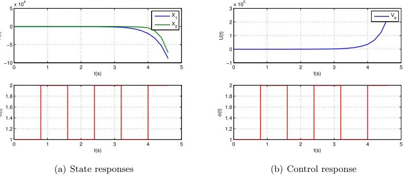
4.9 Responses of the helicopter system withσ= 1 . . . 53
4.10 Responses of the helicopter system with σ= 2 . . . 54
4.11 Responses of the vehicle system with σ= 1 and h= 3 . . . 56
4.12 Responses of the vehicle system with σ= 2 and h= 6 . . . 56
4.13 Responses of the vehicle system with σ= 2 and h= 7 . . . 57
4.14 Output difference betweenh= 6 and h= 7 withσ . . . 58
Acronyms
Acronyms list is the follow:
BMI - Bilinear Matrix Inequalities
HDS- Hybrid Dynamical Systems
LMI - Linear Matrix Inequalities
LPV - Linear Parameter-Varying
LTI- Linear Time Invariant
NCS- Networked Control Systems
SPDLF- Switched Parameter Dependent Lyapunov Functions
Introduction
Hybrid Dynamical Systems (HDS) are systems described by interaction between continuous and discrete dynamic [13] [62]. Switched linear systems are an important class of HDS. They represent a set of linear systems and a rule that orchestrates the switching among them [44].
Goal
General Objective
The principal objective of this project is the design of a robust control law to control switched systems with polytopic uncertainty.
Specifics Objectives
The specifics objectives of the project are:
• Determine the stability of the switched systems through multiple Lyapunov functions.
• Find a stabilizing control signal through state feedback to switched systems with polytopic uncertainty.
• Verify the control laws performance by means of simulation of uncertain delays systems.
HDS overview
Traditionally, the control theory has been focused on the behaviour of continuous or discrete sys-tems. However, many real dynamic systems have hybrid nature [57]. The union between advanced control techniques and hybrid paradigm have been highly successful to deal with problems such as: air traffic control [84], automotive control [4], bioengineering [15], flight control processes [55, 29], road systems [47], manufacturing [17], teleoperated robotic systems [49], robotic assembly tasks, [62], power switching electronic [75], and others.
In the HDS theory, it has been developed important concepts around the stability concepts. Some of these are presented below:
Molchanov and Pyatnitskiy [68] express the stability in terms of cuasi-quadratic Lyapunov func-tions through a theorem that establishes a lineal switched systems stability based on a Lyapunov function for all subsystems. However, from practical point of view, it is difficult to find acceptable
2 LIST OF FIGURES
Lyapunov functions whether analytic or numerically. Liberzon and Morse [58] make a study of the principal problems presented in the stability and design of the switched systems.
Decarlo and Braniky [26] use the Lyapunov stability theory along with LMI theory in order to: 1) guarantee HDS stability and 2) find stability conditions to the switching between controllers of unstable HDS. They are focused on stable and unstable HDS. Braniky analyses the HDS stability and finds a Lyapunov function for each subsystem. They possess switched restrictions to guarantee the global stability of the system. Additionally, Braniky develops some analysis tools applicable to HDS.
In [45], Hetel presents a proposal to solve the synthesis control problem to uncertain switched systems with exponential uncertainty from a point of view of robust control. This can be formulated as a control design to polytopic systems with additive norm bounded uncertainty. Hetel raises a stabilizing control law using LMI conditions that solves the stability problem for these systems.
As Braniky, Hetel [41] makes a stability analysis and a control synthesis to LTI HDS through Lyapunov functions and LMI conditions, but directed to the robust stability and robust control in discrete systems with uncertain parameters and arbitrary switching signal. These systems have parametric uncertainties that are modelled as polytopic matrices. The stability and robust control synthesis based on LMI conditions are applied to the polytopic representation.
Furthermore, Hetel [41] presents two problems in the HDS stabilization topic, the design of a stabilizing switching sequence and of a control law in presence of an arbitrary switching law. A question arises when it searches a stabilizing switching law: Which restrictions must be taken into consideration for the switching law in order to guarantee the switched systems stability? Two restriction types can be considered.
• State space constraints, when the switching law is the control signal.
• Time domain constraints, when it is possible to control only the dwell time for each mode,and when the switching law is arbitrary.
Worldwide some highly prestigious researchers that work with HDS are [11]: Panos Antsakli [3], Michael Branicky [12], Roger Brockett [14], Peter Caines [16], Michael Heymann [46], Wolf Kohn, George Meyer, Sanjoy Mitter [66], Anil Nerode [70], Peter Ramadage [16], Shankar Sastry [81], Pra-vian Varaiya [89], Daniel Liberzon [56], Ivan Malloci [63], Bert van Beek [87], Alberto Bemporad [5], Jamal Daafouz [21], Sebastian Engell [28], Goran Frehse [31], Gerlind Herberich [39], Karl Henrik Johansson [50], Mikael Johansson [50], Rolf Johansson [52], Daniel Lehmann [54], John Lygeros [61], Anders Robertsson [80], Arjan van der Schaft [88], Hans Schumacher [82], Bart de Schutter [83], among others.
LIST OF FIGURES 3
Structure
The structure of this final project is designed in four chapters how is show below.
Chapter 1
The first chapter includes the main concepts of the hybrid dynamical systems field, specially in the switched systems. The stability principles of these systems are declared in order to fully understand the problem. Additionally, the relation between polytopic and switched systems is presented, and the parametric uncertainties are introduced.
Chapter 2
The second chapter is about the robust stability and robust control treated in the context of the switched systems. For this propose, the stability criteria are exposed along with robust control synthesis based on state feedback and output feedback techniques. The chapter develops a less con-servative LMI robust stability tools using Lyapunov functions that take into account the uncertain parameters. This chapter shows also, the switched system representation with uncertainty models, oriented to the stability analysis and control based on linear matrix inequalities. Furthermore, the stability of discrete-time systems with time varying delays is analyzed by using a discrete-time ex-tension of the classical Lyapunov-Krasovskii function. Necessary and sufficient LMI conditions for the existence of such functions are presented. Moreover, in this chapter there are examples for the robust control synthesis and for the switched systems transformation approach are exposed.
Chapter 3
This chapter presents the exponential uncertainty model in switched systems and the mathematical treatment to convert this problem into a polytopic uncertainty model which is intended to apply the LMI robust control synthesis with bounded norm term. This model is represented as a convex polytope for uncertain parameters which are characterized by the delay that appears in the dis-cretization process and by the uncertain and not uniformly spaced in time sampling times. One of the main problems presented is the reduction of complexity when the polytopic representation is used.
Chapter 4
Chapter 1
General concepts of hybrid dynamical
systems
This chapter is presented in three sections: First, definition of Hybrid Dynamic Systems (HDS). Second, an overview of stability theory of HDS with topics related to stability problems in HDS, Lyapunov stability, quadratic stability, global stability and multiple Lyapunov functions for HDS. Finally, it shows the concept and models of uncertainty.
1.1
Definition
Hybrid Dynamical Systems (HDS) are systems described by interaction between continuous and discrete dynamic [13] [62]. The continuous dynamic can be represented by control system of con-tinuous time as a linear system ˙x = Ax+Bu, where the state vector x ∈ Rn, the control input u∈Rm, the dynamic matrix systemA is n×n and the system input matrixB is n×m.
A finite state automata is considered as an example of discrete dynamic as shown in Figure 1.1 with stateqthat takes values in a finite setQ, where the transitions between different discrete states are shot by appropriate values of the input variablev. A hybrid system arises when the input u of a continuous dynamic is any function of the discrete state q. In the same form, the input value v to dynamic discrete is determined by continuous state valuex. For more information about hybrid automata see [64].
A classification of HDS which depends of the state continuity is shown below:
1. HDS without reset maps: its principal feature is the continuity. Namely, state in the previous instant is equal to state in the next instant.
x(t−
) =x(t+)
2. HDS with reset maps: In this case, it presents discontinuity in state
x(t+) =g(t, x−
(t), u(t))
6 CHAPTER 1. GENERAL CONCEPTS OF HYBRID DYNAMICAL SYSTEMS
Figure 1.1: Hybrid dynamical system representation
This classification is shown in figure 1.2.
Figure 1.2: Hybrid dynamical system clasification
Definition 1 [62] A hybrid system is a sextupleH={Q,E,D,G,R,F}, where • Q ={1, . . . , N} is a finite set of discrete state.
• E ⊂Q×Q is a set of edges that defines a source-target relationship between the domains.
• D ={Di}i∈Q is a set of domains where Di is a compact subset of Rn.
• G ={Ge}e∈E is a set of guards, where Ge⊆De(1).
[image:15.612.146.435.424.531.2]1.2. SWITCHED SYSTEMS STABILITY 7
• F ={fi}i∈Q is a set of vector fields such that fi is Lipschitz on Rn.
A hybrid trajectory (in the state space) is described accurately specifying a sequence of its initial conditions, switching times and edges, properly related to the guards and reset maps. The behavior of H allows possible Zeno trajectories. As the reader may notice, the switching conditions (the events) happen due to spacial restrictions on the various domains. Switched systems are a type of HDS, it specifies jumping conditions in time, rather than in the state space [2].
Definition 2 [2] A switched system is a sextuple S ={Q,E,D,G,R,F}, where
• {Q,E,R,F} are characterized in Def. 1.
• D ={Di}i∈Q is a set of domains where Di=Rn.
• G = {0, τ1, τ2, . . .} is a set of guards in time, where τi ∈R+ are increasing in i. Each τi is
mapped to state by a function g:G→Q such that g(g(τi−1), g(τi)) for alli.
A formal representation of the switched systems in continuous time is given by [44]:
˙
x(t) =fσ(t)(t, x(t), u(t)), (1.1) whereσ(t), σ:R+→ I ={1,2,3, . . . , N}represents a piecewise constant function, called
switch-ing signal, that takes values into the set of index I. x(t) ∈ Rn is the state vector of the system, u(t)∈Rm is a command or a control signal, andfi(., ., .),∀i∈ I which are the vector fields describ-ing different modes, notice that there existsN modes available.
In the same way, the switched systems in discrete time are represented by:
x(k+ 1) =fσ(k)(t, x(k), u(k)), (1.2) withσ :Z+→ I.
The switching signal σ(k) (or σ(t) for continuous case) specifies the active system modes or subsystem. The choice of the active subsystem can be based on time criteria, either on state space regions or on the evolution of some physical parameters.
1.2
Switched systems stability
Stability is a property of dynamic systems that evaluates if the system returns to the equilibrium point after it has been disturbed. Formally, the equilibrium pointx∗
is presented when the differ-ential field is null ( ˙x= 0). The equilibrium point could be: 1) stable, 2) asymptotically stable, 3) exponentially stable or 4) global asymptotically stable. For more information see [41].
8 CHAPTER 1. GENERAL CONCEPTS OF HYBRID DYNAMICAL SYSTEMS
In the switched systems stability, Liberzon and Morse [58] have determined three principal problems, which are shown below. They consider a particular case of a LTI piecewise switched system:
˙
x=fσ(x, u) =Aσx+Bσu (1.3)
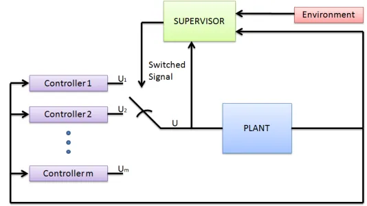
[image:17.612.156.423.259.409.2]Problem A: Find stability conditions such that that the switched system is asymptotically stable for any switching function. An example of this type of problem is the multi-control architecture for a switched system, which is shown in Figure 1.3. It has a supervisor that determines which controller will be connected in close-loop with the plant at each time instant. The supervisor can be switched to any controllers m depending on the system state.
Figure 1.3: Multi-control architecture
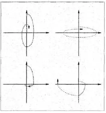
The subsystem stability does not guarantee the system to be globally stable. It depends on the switching. An example of this fact is shown in the Figure 1.4. The top row shows the trajectories of two second order asymptotically stable systems. The bottom row shows the switching system trajectory, left where it is asymptotically stable and left where it is unstable to a switching signal given. For this trajectories, the origin represents the equilibrium point of the system.
Problem B: Given a switching law, determine if the switched system is asymptotically stable. The stability is guaranteed if the switching is sufficiently slow. It is possible that no individual controller can stabilize the plant in a multi-control system, on the other hand, it can be found a switching law in order to have an asymptotically stable switching system.
Problem C: Find a switching law that allows the system be stable.
1.2. SWITCHED SYSTEMS STABILITY 9
Figure 1.4: Possible trajectories to a HDS
Other methods are based on the existence of conditions to the common quadratic Lyapunov functionV(x) =xTP(x)x, which can express through LMI.
Consider the system (1.3), if there exists a matrixP, 0< P =PT, so as to verify the following LMI:
ATi P +P Ai <0,∀i= 1, . . . , N (1.4)
then the quadratic functionV(x) =xTP(x)xis a Lyapunov function for the statement system. It means that the originx= 0 is globally exponentially stable.
When a common quadratic Lyapunov function exists for all subsystems, it can be said that the HDS isquadratically stable. This implies that there exists a scalarǫsuch that:
dV(x)
dt <−ǫkxk (1.5)
In order to verify the stability of HDS of the form (1.3). It is commonly used the Lie algebra approximation proposed by Liberzon in [57, 58].
Different stability criteria exist based on common quadratic Lyapunov functions. However, the existence of this common function is only a sufficient condition but not necessary. Additional, the result of finding this function can be very conservative. For this reason, other type of Lyapunov functions have been taken into account as the multiple Lyapunov functions.
The multiple Lyapunov functions describe a functions family of the form:
V(x) =xTPσ,xx (1.6)
10 CHAPTER 1. GENERAL CONCEPTS OF HYBRID DYNAMICAL SYSTEMS
[image:19.612.143.440.145.314.2]function is that the decrease of the function is only required where the function is active, as it is shown in the Figure 1.5.
Figure 1.5: Multiple Lyapunov functions
Another approximation of multiple Lyapunov functions is presented in the literature. It is based on the concept of Lyapunov-lyke functions. These are families of piecewise continuous and differ-entiable functions. When they are concatenated together, they produce a single non traditional Lyapunov function [76]. It is proposed as Lyapunov-like functions {Vi(x) = xTPix} so that each
vector field Aix(t), i∈ I has its own Lyapunov function. The particularity of Lyapunov-like
func-tions is that the decline of the function is required only when the system is active. A multiple Lyapunov-like function satisfies the following conditions:
• Vi(x) =xTPix is positive definite∀x6= 0 and Vi(0) = 0.
• The derivative of eachVi(x) =xTPix function satisfies the relation
Vi(x) =
∂Vi
∂xAix(t)≤0, ∀i∈ I (1.7)
when the ithsubsystem is active.
A stabilization criterion when a priori knowledge about the switching function has been formu-lated by Johansson [51].
1.3
Relation between polytopic and switched systems
Considering the following polytopic system [44]:
˙
1.3. RELATION BETWEEN POLYTOPIC AND SWITCHED SYSTEMS 11
A(λ(t)) =
N
X
i=1
λi(t)Ai, B(λ(t)) = N
X
i=1
λi(t)Bi
and
λ(t)∈Λ =
(
λ= [λ1. . . λN]∈RN :λi ≥0, N
X
i=1
λi= 1
)
.
The switched linear system
˙
x(t) =Aσ(t)x(t) +Bσ(t)u(t), σ(t)∈ I (1.9) can be expressed as a particular case of a polytopic system withλi parameters restricted to two
discrete valuesλi ∈ {0,1}, such thatλi = 1 whenσ(t) =i.
In order to stabilize this system, it has developed different proposals. A punctual approach is presented in [10], when the switching law is unknown. It uses a LMI static state feedback design method which is based on the existence of a common quadratic Lyapunov function for the close loop system . For this reason, the existence of a symmetric positive definite matrixS and a matrix Y is necessary so as to verify the LMI:
SATi +AiS+BiY +YTBi <0,∀i∈ I (1.10)
Where the common quadratic Lyapunov function is given with the Lyapunov matrix P =S−1.
The state feedback is defined by:
u(t) =Kx(t) withK =Y S−1.
If the switching signal is available in real time, then it can be established a switched state feedback:
u(t) =Kσ(t)x(t) (1.11)
For this case, the solution depends on the existence of several matricesYi as well as the previous
LMI (1.10) is replaced by:
SATi +AiS+BiY +YiTBi <0,∀i∈ I (1.12)
withKi =YiS−1,∀i∈ I.
In discrete time, the approach is based on the use of parameter dependent Lyapunov functions (PDLF) that is a quadratic Lyapunov functions [22]:
V(x) =xT
N
X
i=1
12 CHAPTER 1. GENERAL CONCEPTS OF HYBRID DYNAMICAL SYSTEMS
In PDLF, the Lyapunov matrix depends on the uncertain parameters [85]. In fact, they have been studied to build Lyapunov functions that depends quadratically on the uncertain parame-ters in addition to the state system. If each Lyapunov function exists, it is said the system is bi-quadratically stable.
These functions have applications in robust control domain. These are proposed in order to reduce the conservatism related to uncertainty problems [30, 24].
1.4
Parametric uncertainties
The uncertainty of a switched system implies that dynamic system represented by the matrix A has uncertain parameters due to system variations or because of the parameters being in a way unknown. The stability problem is very complex when parametric uncertainty is considered.
In the discrete time switched linear systems, the uncertain system is given by [44]:
x(k+ 1) = ˆAσx(k) + ˆBσu(k) (1.14)
where ˆAσ represents an uncertain matrix that belongs to the domainAσ ⊂Rnxn, ∀σ∈ I.
Several type of uncertain domains exist, but in order to analyse the switched systems with parametric uncertainties, only three of them will be treated.
• Norm bounded uncertainties, with
ˆ
Aσ ∈ Aσ ={Aσ,0+DσFσ(k)Eσ,kFσ(k)k ≤1} (1.15)
where the Aσ,0 matrices describe a nominal behaviour, Fσ(k) is an uncertain time varying
matrix andDσ, Eσ∀σ∈ I are known matrices.
• Polytopic uncertainties, with ˆ
Aσ ∈ Aσ =co{Aσ,1, Aσ,2, . . . , Aσ,nσ},∀σ∈ I (1.16)
where theAσ,1, Aσ,2, . . . , Aσ,nσ matrices are calledvertex.
• Exponential uncertainties, with
ˆ
Aσ ∈ Aσ =eM ρσBˆσ ∈ Bσ =
Z ρσ
0
eM sdsN (1.17)
whereρσ =tσ+1−tσ is an unknown, bounded, time varying parameter.
Chapter 2
Robust stability and control for
switched systems
This chapter shows the switched system representation with uncertainty models, oriented to the stability analysis and control based on linear matrix inequalities. The construction of Lyapunov functions is one of the most important problems in the control systems theory.
In the theory of robust control, many problems have been solved using the quadratic stability concept. In the continuous time domain some assessments are: 1) A single Lyapunov function supported by Riccati equations [27] or Linear Matrix Inequalities (LMI) [10]. 2) The construction of the parameter dependent Lyapunov functions (PDLF) [24, 30, 35]. 3) The construction of a class of non quadratic Lyapunov functions that is not PDLF and is based on ”smoothing” a polyhedral function for which numerical algorithms are known to exist [6].
In the discrete time domain some approximations are: 1) Robust stability of a class of uncertain discrete time linear systems using PDLF [38]. 2) The construction of PDFL where the parametric uncertainty is time independent which leads to less conservative results than the quadratic stability based ones. Because the results introduce an extra degree of freedom which permits to get a control law without an explicit dependence of Lyapunov matrices [25]. 3) Sufficient conditions to find a bi-quadratically stable system, which means that the construction of a Lyapunov function depends quadratically on the uncertain parameters and quadratically on the system [85]. 4) The extension of results of [25] with polytopic time varying uncertainty, through quadratic PDLF in the system state. In addition, they depend in a polytopic way on the uncertain parameter proposed in [22].
A survey of basic problems in stability and control design of switched systems has been proposed in [59] where it is studied the existence of a switching rule that ensures the stability of the switched systems. The switching sequence can possibly be known whether a priori or not. It has been taken into account the search of a switched quadratic Lyapunov function to check asymptotic stability of the switched systems.
14 CHAPTER 2. ROBUST STABILITY AND CONTROL FOR SWITCHED SYSTEMS
2.1
Robust stability to switched systems
In this section, the theory of robust stability to switched dynamic systems with uncertainties ori-ented to discrete systems is presori-ented.
2.1.1 Stability criteria of polytopic systems
From this moment on, it can be considered a stability result taking into account the PDLF which in this case is used for robust stability analysis applied for switched uncertain systems with poly-topic uncertainty. It is important to say that polypoly-topic time varying systems are systems where the dynamical matrix evolves in a polytope defined by its vertices.
A representation of a uncertain discrete time polytopic systems is given by [44]:
x(k+ 1) =
N
X
i=1
αi(k)Aix(k),
N
X
i=1
αi(k) = 1, αi≥0, ∀i= 1, . . . , N
(2.1)
where x ∈ Rn is the state vector. Besides, αi ≥ 0 is an unknown and bounded time-varying parameter.
The stability of the system (2.1) is checked by PDFL means of the form [22]:
V(k) =xT(k)
N
X
i=1
αi(k)Pix(k), Pi=PiT >0. (2.2)
These functions depend on uncertain parameters αi, ∀i= 1, . . . , N.
A conservative stability criterion based on the classical convex problem is shown in the next theorem.
Theorem 1 System (2.1) is poly-quadratically stable if and only if there exist symmetric positive definite matrices Si, Sj and matrices Gi of appropriate dimensions such that
Gi+GTi −Si GTiATi
AiGi Sj
>0 (2.3)
for alli= 1, ..., N andj= 1, ..., N. In this case, the time varying parameter dependent Lyapunov functions is given by (2.2) with Pi=Si−1.
Applying these concepts to the uncertain switched systems, it can be considered the uncertain switched system
2.1. ROBUST STABILITY TO SWITCHED SYSTEMS 15
where ˆAi:i∈ I withI = 1,2, . . . , N is a family of matrices andσ :Z+ is the switching signal.
ˆ
Aσ(k)(k) is the uncertain matrix:
ˆ
Aσ(k)(k) =
nσ
X
j=1
ασj(k)Aσj, nσ
X
j=1
ασ,j(k) = 1, ασj(k)≥0
where the coefficientsαij describe the polytopic uncertainty of theith mode of the systems. Aσj
denote the extreme points of the polytope ˆAσ andnσ is the number of such points.
2.1.2 Switched parameter dependent Lyapunov function (SPDLF)
Recently, the PDLF have been consider to revise the stability of the switched systems. For in-stance, the switched parameter dependent Lyapunov function (SPDLF) take an important part in the switched state feedback control synthesis at the time the dynamic and the input matrix are simultaneously switched and uncertain.
The system (2.4) is equivalent to
x(k+ 1) =
N
X
i=1
ni
X
j=1
ξi(k)αi,j(k)Aijx(k), (2.5)
with
ξi :Z+→ {0,1}, N
X
i=1
ξ(k) = 1, ∀k∈Z+
Hetel in [44] propose a type of Lyapunov function based on the switched uncertain systems (2.4) and their equivalent representation (2.5) which is described by:
V(k) =xT(k) ˆPσ(k)x(k), with Pˆσ(k) = nσ
X
j=1
ασj(k)Pσj
=xT(k)
N
X
i=1
ni
X
j=1
ξi(k)αij(k)Pij x(k)
(2.6)
wherePij =PijT >0.
The system (2.5) is asymptotically stable if the difference of the Lyapunov function along the solution of the solutions of (2.5)
L=V(k+ 1)−V(k)
satisfies:
L=xT(k)(ATP+A − P)x(k)<0 (2.7)
16 CHAPTER 2. ROBUST STABILITY AND CONTROL FOR SWITCHED SYSTEMS A= N X i=1 ni X j=1
ξi(k)αij(k)Aij,
P = N X i=1 ni X j=1
ξi(k)αij(k)Pij,
P+ =
N X i=1 ni X j=1
ξi(k+ 1)αij(k+ 1)Pij
= N X i=1 ni X j=1
ξm(k)αmn(k)Pmn,
∀k,∀x(k),∀ξi and ∀αij.
Definition 2 [44] The functions (2.6) that satisfy (2.7) are called switched parameter dependent Lyapunov functions (SPDLF) for the system (2.4), also for the equivalent system (2.5).
Theorem 3 [43] A SPDLF can be constructed iff there exist symmetric positive definite matrices
Sij, Snm and matricesGij of appropriate dimension such that:
Gij +GTij−Sij GTijAijT
AijGij Snm
>0 (2.8)
for all i= 1, . . . , N andj= 1, . . . , ni, m= 1, . . . , N andn= 1, . . . , nm. The SPDLF is constructed
with Pij =Sij−1.
2.2
Robust control synthesis for switched systems
The switched state feedback and the switched output feedback are described in this chapter as control synthesis techniques.
In order to treat the robust control synthesis problem of switched systems, the following discrete switching uncertain system will be consider:
x(k+ 1) = ˆAσ(k)x(k) + ˆBσ(k)u(k), (2.9)
where
ˆ Aσ(k) =
naσ
X
j=1
ασj(k)Aσj, naσ
X
j=1
ασj(k) = 1, ασj(k)≥0,
and
ˆ Bσ(k) =
nbσ
X
l=1
βσl(k)Bσl, nbσ
X
l=1
βσl(k) = 1, βσl(k)≥0, ∀k∈Z+
2.2. ROBUST CONTROL SYNTHESIS FOR SWITCHED SYSTEMS 17
represent the uncertainty on the dynamic and input matrix, respectively. σ is consider the switching signal. The uncertain parameters are given by ασj and βσl. Besides, the number of
ex-treme points in the uncertainty ˆAσ and ˆBσ is represented bynaσ and nbσ, respectively.
It is remarkable to say that it is assumed that the switching signal σ is not known a priori. However, it is available in real time for control implementation.
2.2.1 State feedback control
In general terms, the switched state feedback problem can be defined by
Assuming that the switching signal σ(k) is not known a priori but is available in real time for control implementation, the problem of switched state feedback is described by:
u(k) =Kσ(k)x(k) (2.11)
which stabilizes the closed loop system.
The solution problem of the context of robust control can be expressed in the following theorem:
Theorem 4 [43]
There exists a switched state feedback (2.11) stabilizing the system (2.9) if there exists symmetric positive definite matrices Sijl, and Gi, Ri matrices, solutions of the LMIs:
Gi+GTi −Si GiTATij +RTi BilT
AijGi+BilRi Spwv
(2.12)
for all i = 1, ..., N and j = 1, ..., nai, l = 1, . . . , nbi, p = 1, . . . , N, w = 1, . . . , nap and v =
1, . . . , nbp. The switched state feedback control law is then given by
u(k) =
N
X
i=1
ξi(k)Kix(k) (2.13)
with
Ki=RiG−i 1.
The closed loop switched linear system is given by the equation
x(k+ 1) =
N
X
i=1
ξi(k)
nai
X
j=1
αij(k)Aij + nbi
X
l=1
βil(k)BilKi
x(k)
which is equivalent to:
x(k+ 1) =
N
X
i=1
nai
X
j=1
nbi
X
l=1
ξi(k)αij(k)βil(k)Hijlx(k) (2.14)
18 CHAPTER 2. ROBUST STABILITY AND CONTROL FOR SWITCHED SYSTEMS
When the uncertain matrices ˆAσ and ˆBσ depend on a common uncertain parameter, a particular
case of (2.10) with j=l,naσ =nbσ and ασj =βσj, the LMI conditions (2.42) become:
Gi+GTi −Sij GiTATij +RTi BijT
AiGi+BRi Suv
>0 (2.15)
for all i, u = 1, . . . , N, j, v = 1, . . . , naσ, where Sij and Suv are symmetric positive definite
matrices.
2.2.2 Static output feedback control
The control synthesis problem related to the switched static output feedback is
u(k) =Kiy(k) (2.16)
ensuring stability of the closed-loop switched system
x(k+ 1) = (Aσ+BσKσCσ)x(k). (2.17)
This problem is reduced to develop the next LMI and find Pi and Ki,∀i∈ I, such that
Pi (Ai+BiKiCi)TPj
Pj(Ai+BiKiCi) Pj
>0 (2.18)
∀(i, j)∈ I × I.
This is equivalent to find Si,Gi and Ki in the next LMI
Gi+GTi −Si GTi (Ai+BiKiCi)T
(Ai+BiKiCi)Gi Sj
>0 (2.19)
Unfortunately, this problem is non convex in general. For this reason, a sufficient condition is given in the following theorems.
Theorem 5 If there exist symetric matrices Si, matrices Ui andVi such that: ∀(i, j)∈ I × I
Si AiSi+ (BiUiCi)T
AiSi+BiUiCi Sj
>0 (2.20)
and
ViCi =CiSi ∀i∈ I (2.21)
then the output feedback given by (2.16) with
Ki=UiVi−1 ∀i∈ I (2.22)
2.2. ROBUST CONTROL SYNTHESIS FOR SWITCHED SYSTEMS 19
Theorem 6 If there exist symmetric matricesSi, matricesGi, UiandVi(∀i∈ I)such that: ∀(i, j)∈
I × I
Gi+GTi −Si (AiGi+BiUiCi)T
(AiGi+BiUiCi)Gi Sj
>0 (2.23)
and
ViCi =CiGi ∀i∈ I (2.24)
then the output feedback given by (2.16) with
Ki =UiVi−1 ∀i∈ I (2.25)
stabilizes (2.17).
2.2.3 Examples
The following section will introduce two applied examples about the output feedback control of switched systems without uncertainties presented in the previous section. For these examples, it is applied the Theorem 5 as well as the Teorem 6 in order to compare the system response for each control theorem. The examples are simulated in Matlab with SeDuMi toolbox version 1.3.
The first example includes a switched thermostat system that has two switching modes. Due to the natural system behave, each subsystem response is stable.
On the other hand, the second example is related to the lateral dynamic of a vehicle. It is modelled as a linear parameter varying (LPV) system which has a bounded varying parameter. Taking the upper and inner bounds two subsystems are formed, i.e. the LPV system has two modes becoming in a LPV switched system.
Thermostat
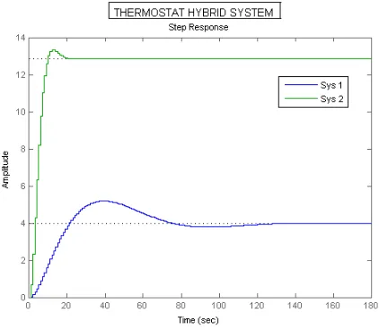
A thermostat system is modelled by hybrid switched system means. It has two modes whose dynamics are represented by following matrices:
A1=
−1 10
−100 −1
B1=
1 0
A2=
−1 100
−10 −1
B2 =
1 0
The discrete step response of the thermostat subsystem is presented in Figure 2.1.
One can notice that both responses of the subsystems are alike to each other. Besides, it also shows that each subsystem is stable.
20 CHAPTER 2. ROBUST STABILITY AND CONTROL FOR SWITCHED SYSTEMS
Figure 2.1: Discrete step response to thermostat subsystems
KT h3 = [ −116.8961 −96.4604 ]
KT h4 = [ −113.9681 −96.9284 ]
The results are shown in Figure 2.2, to the left, it is possible to see the response to Theorem 5 and to the right the control response to Theorem 6.
0 10 20 30 40 50
−0.02 0 0.02 0.04 0.06 0.08 0.1
(a) Response of the theorem 5
0 10 20 30 40 50
−0.02 0 0.02 0.04 0.06 0.08 0.1
(b) Response of the theorem 6
Figure 2.2: Thermostat system states responses
It is appreciated that the switched system are controlled by both theorems. Additionally, the state responses are almost equal.
Lateral dynamic of a vehicle
[image:29.612.92.489.413.580.2]2.2. ROBUST CONTROL SYNTHESIS FOR SWITCHED SYSTEMS 21
following [73]:
• the vehicle is a rigid body;
• flat road;
• the longitudinal motion resistances are ignored compared to wheel lateral forces;
• no rear wheel steering angle;
• the self aligning wheel moments are ignored;
• the steering angle and the vehicle side-slip angle are small enough to employ their linearised expressions;
[image:30.612.198.452.490.597.2]• the vehicle longitudinal speed is a known parameter.
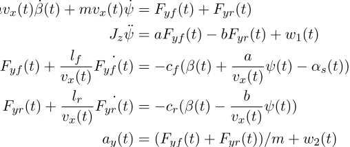
Figure 2.3: Single track model
The system is described by the following set of differential equations:
mvx(t) ˙β(t) +mvx(t) ˙ψ=Fyf(t) +Fyr(t)
Jzψ¨=aFyf(t)−bFyr(t) +w1(t)
Fyf(t) +
lf
vx(t)
˙
Fyf(t) =−cf(β(t) +
a vx(t)
ψ(t)−αs(t))
Fyr(t) +
lr
vx(t)
˙
Fyr(t) =−cr(β(t)−
b vx(t)
ψ(t))
ay(t) = (Fyf(t) +Fyr(t))/m+w2(t)
(2.26)
whereβ is the side-slip angle,ψ(t) is the yaw rate,Fyf(t) andFyr(t) are the front and rear axle
lateral forces,vx(t) is the longitudinal vehicle speed,αs(t) is the steering angle,w1(t) is the process
noise modelled as a torque disturbance,w2(t) is a measurement noise modelled on the lateral
accel-eration output,mis the vehicle mass, Jz is the moment of inertia around the vertical axis,aand b
are the distances between the center of gravity and the front and rear axles, respectively,lf and lr
are the front and rear tire relaxation lengths, and cf and cr are the front and rear axle cornering
22 CHAPTER 2. ROBUST STABILITY AND CONTROL FOR SWITCHED SYSTEMS
Alternatively, the LTI LPV model can be describe as follows:
˙
x=A(m, vx, cf, cr)x+B(m, vx, cf, cr)u+Gnoisew
y=Cx+Du+Hnoisev
where the state space vectorx, the input vectoruand the perturbation vectorware defined by:
xT =
β θ Fyf Fyr
uT =
αs
wT =
w1 w2
The state space representation of this model is
A=
0 −1 m∗1v
x 1
m∗vx
0 0 aj −b
j
−cf∗vx
lf
−cf∗a
lf
−vx
lf 0
−cr∗vx
lr
cr∗b lr 0
−vr
lr B = 0 0
cfvx
lf 0 (2.27) C=
0 1 0 0
The following values of the model parameters have been used for system 1:
m = 1.8865e+003kg, J
z = 2.9667e+003kgm2, a = 1.07m, b = 1.47m, lf = 1m, lr = 1m, cf =
8.0760e+004N mrad,cr= 102690N mrad,vx= 27,77ms.
And for system 2: m = 171.5kg,Jz = 269.7kgm2, a = 1m, b = 1m, lf = 0.5m, lr = 0.5m,
cf = 8.0760e+004N mrad,cr= 102690N mrad,vx= 28ms.
The discrete step response of the vehicle hybrid system is shown in Figure 2.4.
Theorems 5 and 6 were implemented to control this system.The K values are:
KT h3 = [ 0.0366 0.0360 ]
KT h4 = [ 0.0412 0.0410 ]
The control response for systems 1 and 2 using output feedback control with Theorem 5 and Theorem 6 is presented in figure 2.5.
2.3. THE SWITCHED SYSTEM TRANSFORMATION APPROACH FOR SYSTEMS WITH VARYING DELA
Figure 2.4: Discrete step response of vehicle system
Figure 2.5: The output feedback control - Theorem 5 and 6 - Vehicle system
2.3
The switched system transformation approach for systems with
varying delay
The continuous LTI systems with a time varying delay whether dependent and independent have been usual to use the Lyapunov-Razumikhin or Lyapunov-Krasovskii functional method [1, 79]. The advantage of this method is that it can be expressed by LMI conditions [10]. Another proposal to use this method is a numerical approach by means of solution of Ricatti equations [34].
[image:32.612.126.517.314.468.2]24 CHAPTER 2. ROBUST STABILITY AND CONTROL FOR SWITCHED SYSTEMS
Another approach appears in the domain of networked control systems (NCS) that consists in expressing the original problem as a switched system stability problem. It is treated from two views: first, the general switched system transformation [23, 60, 86, 71, 40] and second, the marko-vian jump system [53, 18, 91, 93, 19]. This approach is applied to continuous and discrete systems. Specifically, Nikolakopoulos [86] uses necessary and sufficient LMI conditions for the existence of multiple switched Lyapunov functions [23] in order to analyse the stability of a networked control system.
Strictly, it does not exist a relation between the Lyapunov-Krasovskii approach and the switched system transformation approach, but practically this two stability problems are similar. Hetel [44] establishes a theoretical link between Lyapunov-Krasovskii approach and switched system transfor-mation in the context of discrete time systems with varying time delay wearing multiple Lyapunov functions. Using this transformation approach, the conservatism problem is avoided.
2.3.1 LTI and switched systems with time varying delay
A discrete time system with time delay is described by [44]:
x(k+ 1) =Ax(k) +Adx(k−τ(k))∀k∈Z+
x(k) =φ(k), ∀k∈[−m,0], (2.28)
where x(k) ∈ Rn represents the system state vector at time k ∈ Z+ = {0,1,2, . . .}, τ(k) is a positive integer representing the time varying delay and A, Ad are known constantRn×n matrices.
Here φ(k) is a real-valued initial function on [−m,0] where m > 0. It is assumed that the time varying delay τ(k) is upper-bounded, that is 0< τ ≤m.
For this system, a simple Lyapunov-Krasovskii function is presented by [20]:
Vs(k) =xT(k)P x(k) + m
X
i=1
k−1 X
j=k−i
xT(j)Qx(j). (2.29)
The stability LMI conditions of theVs(k) function are given by following lemma:
Lemma 7 Suppose that there exist possitive definite matrices P and Q such that the following linear matrix inequality (LMI) holds:
P −ATP A−mQ ATP A d
ATdP A Q−ATdP Ad
>0 (2.30)
Then the difference of the Lyapunov-Krasovskii function (2.29) is strictly negative along system (2.28) solutions and the system is uniformly asymptotically stable.
It is remarkable that the LMI founded is only a sufficient condition for the existence of the Lyapunov-Krasovskii function.
2.3. THE SWITCHED SYSTEM TRANSFORMATION APPROACH FOR SYSTEMS WITH VARYING DELA
function in which the Lyapunov matrices are not necessarily related to an unique matrixQ and in which all combinations of delayed states are used in the quadratic forms. Subsequently, thegeneral form of this function is obtained using the sum of all the possible combinations or quadratic forms [42]. The function is expressed by follows:
V(k) =V(k, x(k). . . x(k−m), τ(k)) =
m X i=0 m X j=0
xT(k−i)Pτi,j(k)x(k−j). (2.31)
Where the function involves all the combinations of delayed states with
xT(k−i)Pτi,j(k)x(k−j), i, j ∈ {1, . . . , m}.
Each quadratic form presents different Lyapunov matricesPτi,j(k) which change according to the delay in a set
Pi,j ={P1i,j, P2i,j, . . . , Pmi,j}.
The matricesPτi,j,ı, j ∈ {0, . . . , m}, τ ∈ {1, . . . m}, are defined but not necessarily positive, such
that the function is always positive definite, i.e
V(k) =V(k, x(k). . . x(k−m), τ(k))>0 (2.32) which is the same
Φ(τ) =
Pτ0,0 Pτ0,1 · · · Pτ0,m
Pτ0,1 Pτ1,1 . .. ...
..
. . .. . .. ...
Pτ0,m · · · Pτm,m
>0, (2.33)
where Φ(τ) is a symmetric positive definite matrix for any delayτ in the set{1, . . . , m}. With-out any loss of generality, it may consider thatPτi,j(k) =Pτ(k)i,j T.
The necessary and sufficient LMI conditions for the existence of this functions use augmented state methods. It is necessary to consider other notation as follows:
Λ(τ) =
A Ξ1(τ) Ξ2(τ) · · · Ξm(τ)
I 0 · · · 0
0 I 0 · · · 0
..
. ...
0 · · · 0 I 0
(2.34) with
Ξi(τ) =
Ad, i=τ
0, i6=τ ∀i= 1, . . . , m (2.35)
26 CHAPTER 2. ROBUST STABILITY AND CONTROL FOR SWITCHED SYSTEMS
Theorem 8 [40) The following statements are equivalent:
• There existm·(m+ 1)2 matricesPi,j
τ , τ = 1, . . . , m, i, i= 0, . . . , msuch that the block matrices
Φ(τ), τ = 1, . . . , mdefined by (2.33) satisfy the LMIs
Ξ(τ1) ΛT(τ1)Ξ(τ2)
Ξ(τ2)ΛT(τ1) Ξ(τ2)
>0, (2.36)
for all τ1, τ2 ∈ {1, . . . , m}.
• There exist a delay dependent Lyapunov-Krasovskii function 2.29 whose difference is strictly negative definite along system (2.28) solutions.
The LMIs of Theorem 8 can be extended to the case of discrete time systems with multiple time varying delays such as
x(k+ 1) =Ax(k) +
m
X
i=1
Aix(k−τi(k)), (2.37)
where all the delays τi(k) are varying τi(k) ∈ {1,2, . . . , m},∀i= 1, . . . , m. This generalization
is obtained by reconsidering the notation (2.35) with Ξi(τ1, . . . , m) = Pj, τj(k)=iAj,∀i= 1, . . . , m
and considering as many matrices Λ(τ1, . . . , τm) and Lyapunov matrices Φ(τ1, . . . , τm) as possible
delay combinations.
2.3.2 Equivalence between the switched Lyapunov function and the general de-lay dependent Lyapunov-Krasovskii function
Now, it will be shown that using the multiple Lyapunov function is equivalent to using the general delay dependent Lyapunov-Krasovskii function [44] . For this propose, the following augmented vector is considered:
z(k) = [xT(k). . . xT(k−m)]T, (2.38) the dynamics of the delay system 2.28 can be represented as the following switched system
z(k+ 1) = ¯Aσ(k)z(k). (2.39)
The state matrix ¯Aσ(k) switches in the set of possible matrices {A¯1, . . . ,A¯m} according to the
parameterσ(k). It denotes byI the set of values the switching functionσ(k) may take,σ :Z+→ I. In the cases of time delay systems, the matrices ¯Ai, i∈ I ={1, . . . , m}are given by
A 0 · · · 0 Ad 0 · · · 0
I 0 · · · 0
0 I 0 · · · 0
..
. ...
0 · · · 0 I 0
(2.40)
where the blockAdchanges its positions according toi, such as it is found on the (i+1)thcolumn
2.3. THE SWITCHED SYSTEM TRANSFORMATION APPROACH FOR SYSTEMS WITH VARYING DELA
according to the delay, that is σ(k) =i ifτ(k) =i. The asymptotically stability can be evaluated by using multiple Lyapunov functions [23].
V(k) =zTP¯σ(k)z(k) (2.41)
where ¯P1, . . . ,P¯m are symmetric positive definite matrices. In this case the asymptotic stability
is ensured if the matrices ¯Pi,∀i= 1, . . . , mare solutions of the following LMIs:
¯
Pi A¯Ti P¯j
¯
PjA¯i P¯j
>0, ∀(i, j)∈ I × I (2.42)
In order to analyse the relation between multiple Lyapunov function and Lyapunov-Krasovskii method, Hetel builds the equivalence Lyapunov-Krasovskii function [44]. Sinceσ(k) =iifτ(k) =i, the switched Lyapunov function 2.41 can be expressed as a function that explicitly depends on the delayed variablesx(k), . . . , x(k−m) and the delayτ:
V(k,x¯(k), τ(k)) = ¯xT(k) ¯Pτ(k)x¯(k), (2.43) for allτ(k)∈ {1, . . . , m}. Let ¯Pτ(k)be described by a block matrix similar to the matrix Φ(τ(k))
given in (2.33), for the Lyapunov-Krasovskii approach. It sees that the Lyapunov function is strictly equivalent to the general delay dependent Lyapunov-Krasovskii function (2.29).
In addition, posing Λ(τ) = ¯Aτ for allτ = 1, . . . , m, the LMIs (8) are strictly identically to (2.42).
2.3.3 Control of switched systems with time varying delay
After this theory, it will be consider the closed loop switched systems with time varying delay using a feedback controller. It employs gains that are changed according to the switching law which the switching law is arbitrary.
For this reason, the ”switched system transformation approach” considered in last section is extended to the case of switched systems with time varying delay [44]. Consider the switched delay system:
x(k+ 1) =Aσ(K)x(k) +Bσ(k)u(k−τ(k)), u(k) =Kσ(k)x(k),
x(k) =φ(k), ∀k∈[−θ,¯ 0], σ(k) =ǫ(k), ∀k∈[−θ,¯ 0],
(2.44)
whereσ :Z+→ I ={1,2, . . . , N} represents the switching function, andτ(k)∈ T ={θ, . . . , θ} the time varying delay. Here,φ(k) andǫ(k) represent initial value functions on [−θ,0], whereθ >0 stand for the maximum delay. In the same way, it takes for a minimum delayθ. It is assumed that 0≤θ≤τ(k)≤θ.
Consider ∆ as the minimum dwell time between two switching, the time spent using a wrong switching command depends on the delay τ, i.e. ∆umin =θ and ∆umax =θ. It is inferred that the minimum time spent using the appropriate switching signal is ∆n= ∆−θ.
28 CHAPTER 2. ROBUST STABILITY AND CONTROL FOR SWITCHED SYSTEMS
x(k+ 1) =Aσ(k)x(k) +Bσ(k)Kγ(k)x(k−τ(k)) (2.45)
where γ symbolises the switching function used by the gainsγ :Z→ I, γ(k) =σ(k−τ(k).
Considering the augmented state vector
z(k) = [xT, . . . , xT(k−θ)]T,
the closed-loop system cab be defined by
z(k+ 1) = ( ¯Aσ(K)+ ¯Bσ(k)K¯(γ(k),τ(k)))z(k) (2.46)
where
¯ Aσ(k)=
Aσ(k) 0 · · · 0
I 0 · · · 0
0 I 0 · · · 0
0 · · · 0 I 0
, B¯σ(k) =
Bσ(k) 0 0 .. . 0
(2.47)
¯
K(γ(k),τ(k))=
0 · · · 0 Kγ(k) 0 · · · 0
(2.48)
such that the term Kγ(k) is found on the (τ + 1)th column of ¯K(γ(k),τ(k)). This represents a system that is switched on the original switching function σ(k) and two supplementary switching parameters γ(k) andτ(k). Besides, it can be written as
z(k+ 1) =H(σ(k),γ(k),τ(k))z(k)
with
H(σ(k),γ(k),τ(k))= ¯Aσ(K)+ ¯Bσ(k)K¯(γ(k),τ(k)). (2.49)
If it does not have a dwell time, then the stability of the closed loop cab be verified by checking if there exists positive definite matricesPσ,γτ >0, ∀(σ, γ, τ)∈ D =I × I × T such that:
HiTPjHi−Pi <0,∀i, j∈ D × D. (2.50)
If the minimum time consumed using the good gain is inferior to one sample, ∆n <1. Then,
such condition is the only form to revise the stability. Which means that probably the switching signal in the command is always wrong. The condition may result too restrictive at the time the feedback gainsKγ(k)have to guarantee the decay of the Lyapunov functionV(k) =zT(k)P
(σ,γ,τ)z(k)
2.3. THE SWITCHED SYSTEM TRANSFORMATION APPROACH FOR SYSTEMS WITH VARYING DELA
2.3.4 Examples
In order to illustrate the the results of the switched transformation approach presented in this chap-ter, two examples are exposed in this section.
The examples were developed in Matlab using the Yalmip toolbox with SeDuMi and lmilab solvers. The algorithms implemented to solve each problem are presented below.
2.3.5 Example 1
Considering the system (2.28) introduced by Hetel in [44] with
A=
0.8 0 0 0.97
and Ad=
−0.1 0
−0.1 −0.1
the system is asymptotically stabled for 3 ≤ τ(k) ≤ 5 and 3 ≤ τ(k) ≤ 10, respectively. This results are presented by Gao [36] and Fridman [33]. However, Hetel shows that using the delay Lyapunov-Krasovskii function (2.29) or the switched Lyapunov function (2.41), the system (2.28) is asymptotically stable for 3≤τ(k)≤13. It results are obtained using the LMIs (2.30) and (2.42).
The algorithm developed to verify this case are:
Algorithm:
1. Define the parameters. Insert the system matrices (Ai and Bi) and the number of delays
considered h.
2. Built the A¯i matrices (2.40).
3. Compute the LMI (2.42). The steps to solve this LMI are:
(a) Define the Pi variables
(b) Build the LMI. In order to take into account all possible combinations of the variablePi,
it can be used the nested for loop.
(c) Solve the LMI with SeDuMi or lmilab solvers
4. Verify feasibility of the LMI solution, and the existence ofPi>0.
5. Change the delay value and begin again from second step. Repeat this process until the LMI will be non feasible.
30 CHAPTER 2. ROBUST STABILITY AND CONTROL FOR SWITCHED SYSTEMS
2.3.6 Example 2: Close loop switched system example
This example consider the case of close loop switched systems. It employs the LTI state space model of an inverted pendulum of a cart presented in publication [65].
˙ θ ˙ ω ˙ x ˙ v =
0 1 0 0
(M+m)·g
M·l 0 0 0
0 0 0 1
−m·g
M 0 0 0
· θ ω x v + 0
−M1·l
0 1 M
·u(t), y(t) =
1 0 0 0
· θ ω x v
where M = 2Kg, m = 0.1Kg, l = 0.5m and g = 9.8m/s. The systems is sampled with the sampling period T = 20ms and it is stabilized by a digital state feedback control that is affected by delays:
u(t) =Kx(k−τ), ∀t∈[kT,(k+ 1)T] where
K =
56 12 0.45 1.4
.
Applying the LMIs (2.30) or (2.42), the stability of the discrete system is verified. The algorithm uses to this propose is shown below.
Algorithm:
1. Define the parameters. Insert the systems (Ai and Bi) and the number of delays considered
h.
2. Build the A¯σ(k) and B¯σ(k) matrices (2.47).
3. Build the K¯γ(k),τ(k) matrix (2.48) 4. Determine H(σ(k),γ(k),τ(k)) (2.49).
5. Compute the LMI (2.50). The steps to solve this LMI are: (a) Define the Pi variables
(b) Build the LMI. In order to take in account all possible combinations of the variablePi,
it can be used the nested for loop.
(c) Solve the LMI with SeDuMi or lmilab solvers
6. Verify feasibility of the LMI solution, and the existence of P. It is advisable to evaluate the eigenvalues for the close-loop system
7. Change the delay value and begin again from second step. Repeat this process until the LMI will be non feasible.
For more details about this implementation, see the annex 1.
Chapter 3
LMI Control to discrete switched
systems with polytopic uncertainty
There are several types of uncertainties, in this section they will be presented the exponential un-certainty model in switched systems and the mathematical treatment to convert this problem into a polytopic uncertainty model which is intended to apply the LMI robust control synthesis with bounded norm, where it is represented as a convex polytope for uncertain parameters. This theory is based in Hetel’s developments in [45, 41, 44].
For this work, the delay that appears in the discretization process is the uncertainty. It is rep-resented by sampling timesτ which are uncertain and not uniformly spaced in time.
3.1
Event-based discrete-time representation
Consider the following continuous time LTI system that is controlled by a digital controller
dxc(t)
dt =M xc(t) +N uc(t) (3.1)
where M ∈ Rn×n and N ∈ Rn×m denote the state and the input matrices, respectively,
xc(t)∈Rnrepresents the system state and uc(t)∈Rm the input. The sampling systems is not
uni-form. The digital version of the state is obtained byx(t), which is sent to a computer that produces the digital control u(k). A zero order hold transforms u(k) into a piecewise constant continuous time signaluc(t) =u(t) until a new value is available.
One of the problems presented in these systems occurs when the commanduc(t) may be affected
by delays which are time-varying and possible unknown. They may be greater than the sampling period and they may have a very large variation. This phenomenon is very difficult to model. Usu-ally, it is modelled over a sampling period (99,101]. However, this representation is not appropriate for treating the delay variations larger than a sampling period. Because, the system input uc(t)
may change its value several times during the same sampling period.
The typical discrete time representation over a sampling period is given by:
32CHAPTER 3. LMI CONTROL TO DISCRETE SWITCHED SYSTEMS WITH POLYTOPIC UNCERTAINTY
x(k+ 1) =eM Tx(k) +
Z τkmax−1(k)
KT
eM[(k+1)T−s]dsN u(k−k
max) +. . .
. . .+
Z τ0(k)
τ1(k)
eM[(k+1)T−s]dsN u(k−1) +Z (k+1)T
τ0(k)
eM[(k+1)T−s]dsN u(k)
(3.2)
This model is very complex because it has kmax+ 1 non-linear uncertain exponential matrices,
each one depending on different unknown time-varying parameters τj(k). For this representa-tion, it is assumed that during the kth sampling cycle, the command may take values in the set
{u(k), u(k−1), . . . , u(k−kmax)}. Additionally, it is considered a constant sampling periodT. The
instant of the time the commandu(k−1) occurred during thekth sampling period is represented by τj(k), withkT ≤τj(k)≤(k+ 1)T, j = 0, . . . , k
max.
Hetel proposes in [44] a event-based discrete-time representation. It is possible to model both time varying delays and non-uniform sampling systems. Two possible events occur in the control loop: sampling event, representing the fact that new systems data are taken for control compu-tation, and actuation event, reflecting the different input changes. These events are distinct and happens at non uniform time intervals in an arbitrary way. It is possible that several actuations occur between two sampling events or no actuation at all.
The evolution between two events is described by:
xc(ti+1) =eM ti+1−tixc(ti) +
Z ti+1−ti 0
eM sdsN uc(ti), (3.3)
where ti, i ∈N represents the instants of the time when such events occur. It may correspond
to the τj(k) parameter in model (3.2). The model decomposes the behaviour of the systems (3.1) and (3.2) on time intervals for which the command is constant.
The command uc(ti) depends on a sample xc(ti) with ti ≥tj. Let ρi denotes the time interval
between two successive events. ρi is unknown, bounded, time varying parameter, i.e. :
0< ρ < ρi =ti+1−ti ≤ρ.
Introducing the following notation
ηi =xc(ti), and ui =uc(ti) (3.4)
where they express the state and input vector, respectively, at the moment when an event occurs. Using this notation, system (3.3) can be represented as a discrete time uncertain system withexponential uncertainty as follows:
ηi+1=A(ρi)ηi+B(ρi)ui (3.5)
where exponential uncertainty is:
A(ρi) =eM ρi, B(ρi) =
Z ρi
0
3.2. MODELLING OF SWITCHED EXPONENTIAL UNCERTAIN SYSTEM AS A POLYTOPIC UNCERTAIN
Stabilizing a system affected by timing problems is the same as finding a control for system (3.5). If it is considered the case where the control signal uc(ti) is a function of past values of the
digital system state,
uc(ti) =Kxc(tj) =Kxc(ti−θi), θi∈ T ={θ∈Z
+:θ≤θ≤θ}
where θi = i−j represents the distance between the sampling and actuation in the space of
the events. It is bounded positive integer. As a result, the input vector ui of the system (3.5) is
equivalent to
ui =Kηi−θi
from which the close loop system is an uncertain system with exponential uncertainty and time varying delay in the state.
3.2
Modelling of switched exponential uncertain system as a
poly-topic uncertain model
Extending the results to the switched systems, the system (3.5) can be written as equation (3.6) where a switched uncertain system with exponential uncertainty is represented. This system can represent digital models for a network controlled systems or systems affected by sampling jitter [45].
x(k+ 1) =Ai(ρ(k))x(k) +Bi(ρ(k))u(k),
Ai(ρ(k)) =eMiρ(k), Bi(ρ(k)) =
Z ρ(k)
0
eMiρ(k)sdsN
i,
(3.6)
where{Mi∈Rn×n:i∈P}and{Ni∈Rn×m :i∈P}are two families of matrices that represent
the system in continuous time. Each pair (Mi, Ni), i∈P describes a different regime of system
be-haviour. Here, the uncertain parameter ρ(k) is positive, time varying and bounded, 0< ρ < ρ(k). Otherwise, the switching signali:R+ →P ={1,2, ..., n}, that indicating the active system regimen.
For the control problem to be treatable, the exponential uncertainty model must be changed into a polytopic uncertainty model. For this purpose, it is used a h-order Taylor series expansion. Using it, the exponential uncertaintiesAi(ρ(k)) andBi(ρ(k)) can be express as matrix polynomials
with additive terms that can be bounded. This expansion method makes possible to find a convex polytope with an equivalent number of vertices to the Taylor order. This polytope involves the polynomial matrix.
Proposition 9 [44] Through Taylor series and basic properties of matrix exponentials, it is possible to express system (3.6) as:
34CHAPTER 3. LMI CONTROL TO DISCRETE SWITCHED SYSTEMS WITH POLYTOPIC UNCERTAINTY
where
Ahiρ(k) =
h
X
j=0
Mij k! ρ
j(k) and
Bihρ(k) =
h
X
j=0
Mij−1 k! ρ
j(k)N i
are polynomials that represent the h-order Taylor series approximation of system (3.6) matrices and
∆Ahiρ(k) =eMiρ(k)−
h
X
j=0
Mij k! ρ
j(k) and
∆Bhiρ(k) =
Z ρ(k)
0
eMisdsN
i− h
X
j=0
Mj−1
i
k! ρ
j(k)N i
(3.8)
are the remainders of the approximation.
Below, it is determined how polynomial matrices with positive parameters can be bounded by convex polytopes. Usually, any h-degree polynomial
L(ρ) =L0+ρL1+ρ2L2+...+ρhLh, (3.9)
with a ρ parameter positive and bounded in a closed interval. It can be bounded by a convex polytope with 2hvertices, a hyper-rectangle. In this situation, it is possible to find a convex polytope with only h+ 1 vertices inside the hyper-rectangle that gives a tigther approximation of the Taylor series polynomial. The polytopic form of the uncertain parameters system of the system is defined by the following lemma.
Lemma 10 [41] Consider the uncertain parameter dependent polynomial matrix (3.9) such that the uncertain parameter ρ is bounded and positive: 0 < ρ < ρ < ρ. Then, one can find a convex polytope with h+ 1 vertices that envelopes the polynomial matrix L(ρ), i.e. there exists parameters
µj(ρ),
h+1 X
j=1
µi(ρ) = 1, µi(ρ)>0 ∀j= 1, ..., h+ 1
such that
L(ρ) =
h+1 X
j=1
µi(ρ)Uj (3.10)
3.2. MODELLING OF SWITCHED EXPONENTIAL UNCERTAIN SYSTEM AS A POLYTOPIC UNCERTAIN
U1 =Lhρh+Lh−1ρh−1+. . .+ρ2L2+ρL1+L0,
U2 =Lhρh+Lh−1ρh
−1+. . .+ρ2L
2+ρL1+L0,
U3 =Lhρh+Lh−1ρh−1+. . .+ρ2L2+ρL1+L0,
.. .
Uh+1 =Lhρh+Lh−1ρh−1+. . .+ρ2L2+ρL1+L0.
(3.11)
The relationship between the uncertain parametersρ and µare given by:
µ1= 1−
ρ−ρ
ρ−ρ, µj =
ρj−1−ρj−1
ρj−1−ρj−1 −
ρj−ρj
ρj−ρj, j= 2, . . . , h+ 1 (3.12)
For the proof of the lemma see [44] and [45].
Employing the classical Gauss method, the solution can be computed the recursive formula:
µ1 = 1−
ρ−ρ
ρ−ρ, (3.13)
µj =
ρj−1−ρj−1
ρj−1−ρj−1 −
h+1 X
l=j+1
µl, j = 2, . . . , h (3.14)
It is possible to prove that
µj =
ρj−1−ρj−1
ρj−1−ρj−1 −
ρj−ρj
ρj−ρj, j = 2, . . . , h+ 1 (3.15)
which is strictly positive since the functionf :R→R
f(x) = ρ
x−ρx
ρx−ρx
is monotone decreasing forx∈(0,∞). Therefore,Uidefine a convex polytope that includesL(ρ).
Remark. The previous lemma gives not only a method for reducing the number of vertices of the polytope to which the polynomial matrix belongs, but also indicates a tighter approximation of the polynomial uncertainty. It means that instead of taking the complete 2h hyper-rectangle, it considers only the h+1 convex polytope to which the uncertainty effectively belongs.