Influence of the loss of time-constants repertoire in pathologic heartbeat dynamics

Physica A 348 (2005) 304–316

Influence of the loss of time-constants repertoire

in pathologic heartbeat dynamics

L. Guzma´n-Vargas

, A. Mun˜oz-Diosdado

, F. Angulo-Brown

a_{Unidad Profesional Interdisciplinaria en Ingenierı´a y Tecnologı´as Avanzadas, Instituto Polite´cnico} Nacional, Av. IPN No. 2580, L. Ticoma´n, Me´xico D.F. 07340, Me´xico

b_{Unidad Profesional Interdisciplinaria en Biotecnologı´a, Instituto Polite´cnico Nacional, Av. Acueducto s/n,} L. Ticoma´n, 07340 Me´xico D.F., Me´xico

c_{Departamento de Fı´sica, Escuela Superior de Fı´sica y Matema´ticas, Instituto Polite´cnico Nacional, Edif.} No. 9 U.P. Zacatenco, Me´xico D.F. 07738, Me´xico

Received 25 June 2004; received in revised form 30 July 2004 Available online 27 October 2004

Abstract

We present a fractal analysis of diurnal heart interbeat time series from healthy young subjects and patients with congestive heart failure. We describe some differences between these groups by means of the calculation of some scale-invariant exponents. A previous simple model to reproduce the observed differences is briefly described (Phys. Rev. E 67 (2003) 052901). The model is based in first-order autoregressive processes and consists in the combination of time constants. We suggest that some changes occurring with disease could be related to the participation or absence of time constants. Finally, we also present a multifractal analysis of simulated sequences and their comparison with real data.

r2004 Elsevier B.V. All rights reserved.

PACS:87.19.Hh; 87.10.+e; 89.20.a

Keywords:Time series; Heart rate dynamics; Time constants

www.elsevier.com/locate/physa

0378-4371/$ - see front matterr2004 Elsevier B.V. All rights reserved. doi:10.1016/j.physa.2004.09.019

_{Corresponding author. Current address: Department of Chemical and Biological Engineering,}

1. Introduction

Scaling and fractal properties of many real time series have attracted the attention of researchers from different disciplines[1,2]. In this sense, global and local invariant quantities have been widely used to describe both the monofractal and multifractal properties of several irregular and nonstationary signals. It has been suggested that changes in scale-invariant quantities related to correlations in heart rate variability are processes occurring with aging and some heart failures. Of interest is the change in the self-organization (fractal) that has been related both to the apparition of crossovers in the value of some scale-invariant quantities [3–6] and to the loss of multifractality with disease [7]. For example, Goldberger et al. [8] discuss that alterations in scaling behavior associated with physiologic aging exhibit different patterns than those observed in heart failure patients. In fact, the hinges present in the crossover region from both the elderly healthy individuals and the patients with congestive heart failure (CHF) are in opposite directions[8]. In previous works[3,8], by means of monofractal approaches such as detrended fluctuation analysis (DFA), it has been reported that for data from healthy young subjects the DFA-exponent (g) is close to 1, that is, with long-range correlations as in 1=f noise. For heart failure data, two regions were described, over short scales, the fluctuations resembled white noise (gclose to 0:5) and over large scales,gis 1:3;a value close to Brownian motion (g¼1:5). Multifractal studies have revealed that healthy heartbeat (R–R series) dynamics is more complex than under heart failure conditions [7]. This loss of multifractality have opened new questions about the mechanisms involved in the neuroautonomic control of heart rate. An important question is how to reproduce the crossover behavior observed in heart failure (upward open hinges) under monofractal approaches and also to be in agreement with the loss of multifractality. In a recent work[5], a simple model of the aging effect on heart interbeat series was described. This model suggests that aging is probably related to the heart’s loss of repertoire of responses to environmental stimuli. The model is based in a combination of noisy first-order autoregressive processes, each one with a single characteristic time of correlation. In the present paper, based in this same model, we now reproduce the crossover behavior observed in RR-time series of CHF patients, that is, the upward open hinges in the crossover region. The paper is organized as follows: In Section 2, we introduce a resume of the methods employed in the analysis. In Section 3, results of the analysis of heartbeat series from healthy subjects and CHF patients are presented. In Section 4, we show some simulations and their comparison with real data. Finally, we discuss our results in Section 5.

2. Methods

2.1. Higuchi method

Higuchi proposed a method to calculate fractal dimension of self-affine curves in terms of the slope of the straight line that fits the length of the curve versus the time interval (the lag) in a double log plot. The method consists in considering a finite set of data taken at an interval n1;n2;. . .;nN: From this series we construct new time

series, nk

m;defined as

nðmÞ;nðmþkÞ;nðmþ2kÞ;. . .;n mþ Nk k

k

;

with m¼1;2;3;. . .;k; ð1Þ

where [ ] denotes Gauss’ notation, that is, the bigger integer andmandkare integers that indicate the initial time and the interval time, respectively. The length of the curvevk_m;is defined as

LmðkÞ ¼

1 k

XNkm

½

i¼1

jnðmþikÞ nðmþ ði1ÞkÞj 0

@

1 A N_Nm1

k

k 2

4

3

5 (2)

and the term ðN1Þ=½ðNmÞ=kk represents a normalization factor. Then, the length of the curve for the time intervalkis given byhLðkÞi: the average value overk setsLmðkÞ: Finally, ifhLðkÞi /kD;then the curve is fractal with dimension D[9].

The fractal dimension is related to the spectral exponentbby means ofb¼52D

[9]. Note that this relationshipis valid for 1oDo2 and 1obo3:

2.2. Detrended fluctuation analysis

Peng et al. [10] introduced detrended fluctuation analysis (DFA) to detect correlations in irregular and nonstationary signals. The DFA method is based on the classical random walk variations. To illustrate DFA, we depart from an initial time seriesBðiÞ(of lengthN), first, this series is integrated,yðkÞ ¼Pk_i¼1½BðiÞ Bave;after

doing this, the resulting series is divided into boxes of sizen. For each box, a straight line is fitted to the points, y_nðkÞ: Next, the line points are subtracted from the integrated series, yðkÞ; in each box. The root mean square fluctuation of the integrated and detrended series is calculated by means of

FðnÞ ¼

ffiffiffiffiffiffiffiffiffiffiffiffiffiffiffiffiffiffiffiffiffiffiffiffiffiffiffiffiffiffiffiffiffiffiffiffiffiffiffiffiffiffi 1

N XN

k¼1

½yðkÞ y_nðkÞ2 v

u u

t ; (3)

this process is taken over several scales (box sizes) to obtain a power-law behavior FðnÞ /ng_{;withgan exponent which reflects self-similar properties of the signal. It is}

2.3. Multifractal method

The behavior of a nonlinear dynamical system can be often characterized by fractal or multifractal measures. Multifractal signals require many local exponents to fully characterize their scaling properties [11]. The multifractal distributions are characterized by the functionfðaÞ(Fractal dimension) againsta(Ho¨lder exponent) that is called the multifractal spectrum[12]. Here, we use the method proposed by Chhabra and Jensen [13] that provides a highly accurate, practical and efficient method for direct computation of the singularity spectrum fðaÞ: Briefly, we can consider a normalized time series as a singular measurePðxÞ:First, we calculate the fðaÞ curve covering the measure with boxes of length L and computing the probabilities PiðLÞ in each box. Next, we construct the one-parameter family of

normalized measures given by

m_iðq;LÞ ¼ ½PiðLÞ

q

P

j½PjðLÞq

; (4)

withqtheqth moment of the measure. Finally, for each value ofq, we evaluate the numerators on the right-hand sides of the following equations:

fðqÞ ¼ lim

L!0

P

imiðq;LÞlnm_{ðq;LÞ

lnL ; (5)

aðqÞ ¼ lim

L!1

P

imiðq;LÞln½P_{ðLÞ

lnL : (6)

These equations provide a relationship between a Hausdorff dimension f and an average singularity strengthaas implicit functions of the parameterq. The plot off versusais the multifractal spectrum. The mass exponenttðqÞ[12]is given in terms of theaðqÞand the fractal dimensionfðaðqÞÞby

tðqÞ ¼qaðqÞ fðaðqÞÞ: (7)

The curve fðaÞ characterizes the measure and is equivalent to the sequence of mass exponents tðqÞ: We also can describe the measure with the generalized fractal dimensions Dq introduced by Grassberger and Proccacia [14], which is

given by

Dq ¼

tðqÞ

1q ; (8)

where the numeric factor 1qmodifies the mass exponent to give the resultDq¼E

for the sets of constant density in anE-dimensional space.

3. Data analysis

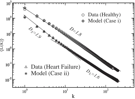
For our study we consider diurnal periods of ECG records (approximately 8 h). We calculate the fractal dimension by means of the Higuchi method. In Fig. 1, we present the Higuchi analysis of one representative case of each group. For the healthy group, we find that a single fractal dimension value is needed to fit the data. The scaling exponent associated with healthy subjects is D¼1:8160:029 (mean valueSD). This exponent is close to the value previously reported for the healthy young group [5,6] for very short sequences and is consistent to that reported by means of DFA, confirming that long-range correlations are present in healthy heartbeat data. For the heart failure group, we find for 10 of 11 sets, a clear crossover behavior in the fractal dimension Dvalue. In the region of short scales (ko12), the scaling exponent isDS ¼1:8950:063;whereas for large scales (k412),

DL¼1:6570:044: Student’s t-test confirms significant differences between these

regions (P¼0:0001). For very short scales there is a tendency to white noise and for large scales the walker is close to Brownian motion. Of interest is that this crossover is not present in all samples. But in the average there is a tendency to Brownian motion of heart failure data-set at large scales. On the other hand, we also apply the DFA method to the same records, we observe that the scaling exponent related to healthy subjects is: g¼1:0270:063: For the CHF groupwe find the following scaling exponents:g_S¼0:8480:19 andg_L¼1:2220:056;where the subscriptsS andLrepresent short and large scales, respectively. As we described in the Section 2, a simple relationship can be stated between the Dand thegof the DFA method,

g¼3D:Using the values ofDreported above and this simple equation, we obtain the equivalent values of the DFA-exponent (ge_{). For the healthy groupwe getg}e_¼

1:184;which is in reasonable agreement with theg-value calculated by means of the DFA-algorithm.

100 101 102

k

10-2 100 102

〈

L(k)

〉

Healthy Heart Failure

slope =1.81 slope=1.9

slope=1.6

4. Simulations and analysis

4.1. The autoregressive model

According to the model described in Ref.[5], an autoregressive process is given by

Xtþtþ1¼aXttþett; (9)

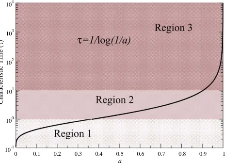
where is a Gaussian distributed random variable and a is a coefficient in the interval 0pap1: Time constants are related to the correlation function as the characteristic time in which the correlation has decayed 1=e:The time constant can be related to the coefficient a through t¼1=lnð1=aÞ; clearly tgoes from zero to infinite whilea varies from 0 to 1.

As it has been suggested[5], healthy heartbeat dynamics can be described, in a first approximation, as the participation of many time constants given by processes of the type of Eq. (9). The sum of many power spectra each one with a single characteristic timetis of the form,

SðfÞ ¼

Z 1

0

dtsðfÞPðtÞ; (10)

wheresðfÞis the power spectrum of one autoregressive process (Eq. (9)),

sðfÞ ¼ 4At

1þ ð2pftÞ2 ; (11)

with Aa constant and PðtÞ is the distribution of time constants. Briefly, it is well known that if PðtÞ is of the form PðtÞ ¼1=t; integration of Eq. (10) leads to 1=f behavior over certain region[5,17]. Now, if we assume thatPðtÞis the contribution ofNtime constants we can expressPðtÞas

PðtÞ ¼ 1

N Xi¼N

i¼1

dðttiÞ: (12)

4.2. Monofractal analysis

ultra low frequencies (ULF; fo0:03 Hz), ULF has been associated to thermo-regulation and other long-term processes [19,21]. For our study we generate time series of 32,000 points. We find that a good approximation to real data (healthy subjects) can be obtained with a superposition of at least 18 time constants (Case i) from the three main regions described above[5]: six from each region. Using DFA we calculate the scaling exponent of the generated signal and find that the slope is

g¼1:010:04 (seeFig. 3).

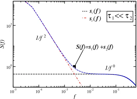
On the other hand, as described in the previous section, heart failure data reveals a crossover that leads to two separated regions, over short scales is close to white noise and for large scales is close to Brownian motion. In order to recover the mentioned crossover, here, we suggest a quite different superposition of time constants. For example, consider the influence of two extremal time constants t1; t2 with t15t2:

The linear superposition of these two characteristic times can be calculated according to Eqs. (10) and (12), the result is,

SðfÞ ¼ 2At1

1þ ð2pft1Þ2

þ 2At2 1þ ð2pft2Þ2

: (13)

This power spectrum reflects two regions (see Fig. 4). For short frequencies the slope is Brownian-type, whereas for large frequencies it is close to white noise. According to this, we consider a superposition of some extremal time constants, that is, only considering the influence of time constants from both the Region 1 and the Region 3. From the Region 1 we take at least 6 very short time constants and from the Region 3 we take at least 3 very large time constants (Case ii). We observe that the superposition of 6 time constants in the interval½0:33;0:52(Region 1) and 3 time constants from the Region 3, leads to a crossover behavior in the simulated data.

0 0.1 0.2 0.3 0.4 0.5 0.6 0.7 0.8 0.9 1

a

10-1 100 101 102 103 104

Characteristic Time (

τ)

However, a better approximation to the crossover observed in real data (seeFigs. 3

and5) was obtained by considering the accentuation of the term corresponding to the time constant t _{¼0:52; this value roughly corresponds to the well-known}

0 1 2 3 4

log n -2

0 2

log F(n)

slope=1

10

10

Data (Heart Failure) Model (Case ii)

0 1 2 3 4

log n -2

0 2

log F(n)

Data (Healthy) Model (Case i)

slope=0.6

slope=1.3

Fig. 3. DFA-plots of logFðnÞ vs. logn for data from both one healthy subject (open circles) and its simulation (Case i), and one CHF-patient (open triangles) and its simulation (Case ii). For the healthy group(above) the slope is close to one. For the heart failure group(below), over short scales the slope is close to 0:5 (uncorrelated noise) whereas for large scales the slope is 1:3;close to the Brownian motion value (1:5). The simulation of the Case (i) was carried out as follows: we took six time constants from each region, from Region 1: t¼0:39;0:41;0:43;0:62;0:83;1:09; from Region 2: t¼ 1:44;1:95;2:80;4:48;9:49;10:63; from Region 3: t¼19:49;49:49;99;999;9999: For the Case (ii) we consider 6 time constants from the Region 1:t¼0:33;0:37;0:39;0:41;0:45;0:52 and 3 time constants from Region 3:t¼99;999;9999:We accentuated the participation of the time constantt_{¼0:52;multiplying}

the term by the factor 5.

10-5 10-4 10-3 10-2 10-1

f

100 102

S(f)

2

s ( f ) s ( f )

1/f

1/f0

1 2

S(f)=s (f) +s (f)

τ << τ

oscillation that is synchronous with respiration (f 0:25 Hz) [22]. In Fig. 3 we show a comparison of both real and simulated data under the DFA method. InFig. 5, results of the Higuchi analysis are presented for the same cases. A good agreement between the model and real data is observed.

4.3. Multifractal analysis

The multifractal formalism has been applied by Ivanov et al.[7,15]to the analysis of the human heartbeat. They found that multifractality in the heartbeat interval records of healthy subjects cannot be attributed to the activity of the subjects or to the sleep-stage transitions. In contrast, they found that the heartbeat data from subjects with congestive heart failure show a clear loss of multifractality, that is, the width of the multifractal spectra for healthy subjects is greater than those associated with subjects with pathological conditions. To robust our study, we applied the multifractal analysis to the generated time series for the cases described in the previous section. InFig. 6, we present the multifractal spectra of our analysis. Our results show that, for the simulation (Case i) a broad multifractal spectrum is observed as reported for healthy subjects[7]. In contrast, the CHF-simulation (Case ii) leads to a narrow multifractal spectrum (see the inset of Fig. 6). This finding suggests that the absence of some characteristic times could be related to the loss of complexity of the signal as observed in CHF patients[7,18]. Next, we calculate the spectrum of generalized fractal dimensions Dq [14]. In Fig. 7 we show that, for

healthy subjects and their simulation, Dq is a nonlinear function, indicating the

multifractality of the signals. In contrast, for CHF patients and their simulation,Dq

10-2 10-1 100 101 102 103 〈〉

100 101 102

k 10-2 10-1 100 101 102 103 D=1.8 D =1.9

D =1.6

Data (Heart Failure) Model (Case ii)

10-2 10-1 100 101 102 103 〈 L(k) 〉

100 101 102

k 10-2 10-1 100 101 102 103 S L Data (Healthy) Model (Case i)

is almost flat, indicating monofractality. Clearly both groups are separated. The narrow multifractal spectrum for the CHF patients inFig. 6is reflected in the flatDq

spectrum inFig. 7.

4.4. Discussion

Our simple procedure permits to describe the apparition of the crossover as a reduction of repertoire of time constants. Interestingly, this reduction is presented in

0.99 0.995 1 1.005 1.01

α

0.9 1

f(

α)

Data (Heart Failure) Model

Data (Healthy) Model

0.95 1 1.05 1.1

α

0.2 0.3 0.4 0.5 0.6 0.7 0.8 0.9 1

f(

α)

Data (Healthy) Simulation (Case i) Data (Heart Failure) Simulation (Case ii)

Fig. 6. Multifractal spectra of real data (Healthy subjects and CHF patients) and their comparison with simulations (Cases i and ii). Healthy groupand its simulation (Case i) displays a broad multifractal spectrum whereas CHF patients and their simulation (Case ii) show a narrow spectrum (see the inset).

-30 -20 -10 0 10 20 30

q

0.96 0.97 0.98 0.99 1 1.01 1.02 1.03 1.04 1.05

Dq

Data (Healthy) Simulation (Case i) Data (Heart Failure) Simulation (Case ii)

Fig. 7. The spectrum of generalized fractal dimensionsDqas a function of the moment orderqfor real

data (healthy subjects and CHF patients) and its comparison with simulations. CHF patients and their simulation show a flatDqfractal spectrum compared with theDqspectrum of healthy subjects and their

a very different manner to that occurring with healthy elderly data[5]. In the present case, the reduction consists in removing the intermediate region (intermediate time constants), but preserving the regions of very short and very large time constants. This is consistent with some studies that have reported an absence of LF variability of sympathetic nerve activity in severe heart failure [22] and a disturbed sympathetic–parasympathetic balance in pathologic conditions [22,23]. Although this simple model does not relate the parameters to specific neuroautonomic mechanisms, it attempts to reproduce the general features of heart failure data. Particularly, the simulation reveals that under failure conditions the output, for very short scales, is close to uncorrelated behavior whereas for large scales is close to a random walk (the sum of uncorrelated events), indicating the apparition or accentuation of some characteristic times and the inhibition or reduction of intermediate scales. On the other hand, multifractal analysis of simulated data reveals that loss of time constants repertoire is probably related to the loss of multifractality. The change in shape of thefðaÞcurve in relation with the loss of time constants may suggest a simple form of evaluation of complexity under heart failure conditions.

As a final discussion, it is important to clarify the differences between the methods used in this work. We have used separately monofractal and multifractal methods to the assessment of scaling properties of heartbeat time series. As it has been pointed out[24], the methods like DFA and Higuchi are more appropriated to the study of monofractal signals characterized by a single scale exponent. One of the advantages of monofractals methods like DFA is the assessment of correlations present in the signals. In contrast, multifractal signals require an infinity number of indices to describe their scaling properties[7,24]. The singularity spectrum,fðaÞ;quantifies the fractal dimension of a sub-set characterized by the local exponenta:In this sense, multifractal signals are more complex than monofractal ones. In the case of beat-to-beat interval, it is reasonable to assume that this variable is a multifractal signal

[7,24]. As it was described by Ivanov et al. [7] and here, the healthy heartbeat is characterized by a broad multifractal spectrum. In contrast, heart failure conditions leads to a narrow spectrum. This change in the spectrum has been related to a reduction of anticorrelations under CHF conditions[7,15].

5. Conclusions

constants do not participate in the obtaining of the upward open hinge-shaped log–log plots (both in DFA and Higuchi methods) corresponding to this kind of patients. Interestingly, the simple model leads to a narrow multifractal spectrum as observed in real data, suggesting that the participation or absence of time constants could be very important to understand the loss of complexity in heartbeat time series. In summary, our simple loss of time repertoire-model reasonably reproduce the statistical behavior of both healthy young and elderly individuals [5] and also that of CHF patients.

Acknowledgements

We thank M. Santilla´n for stimulating suggestions and E. Calleja for fruitful discussions. This work was supported by EDI-IPN and COFAA-IPN.

References

[1] S. Buldyrev, A. Goldberger, S. Havlin, C.K. Peng, H.E. Stanley, Fractals in Biology and Medicine: from DNA to Heartbeat, Springer, Berlin, 1994.

[2] J.B. Bassingthwaigthe, L.S. Liebovith, B.J. West, Fractal Physiology, Oxford University Press, New York, 1994.

[3] C.K. Peng, S. Havlin, H.E. Stanley, A.L. Goldberger, Chaos 5 (1) (1995) 82–87.

[4] N. Iyengar, C.-K. Peng, R. Morin, A.L. Goldberger, L.A. Lipsitz, Am. J. Physiol. 271 (1996) R1078–R1084.

[5] L. Guzma´n-Vargas, F. Angulo-Brown, Phys. Rev. E 67 (2003) 052901.

[6] L. Guzma´n-Vargas, E. Calleja-Quevedo, F. Angulo-Brown, Fluctuation Noise Lett. 3 (1) (2003) L81–L87.

[7] P.Ch. Ivanov, L.A.N. Amaral, A.L. Goldberger, S. Havlin, M. Rosenblum, Z.R. Struzik, H.E. Stanley, Nature 399 (1999).

[8] A.L. Goldberger, L.A.N. Amaral, J.M. Hausdorff, P.Ch. Ivanov, C.K. Peng, H.E. Stanley, Proc. Nat. Acad. Sci. USA 99 (Supp. 1) (2002) 2466–2472.

[9] T. Higuchi, Physica D 31 (1988) 277–283; T. Higuchi, Physica D 46 (1990) 254–264.

[10] C.K. Peng, J. Mietus, J.M. Hausdorff, S. Havlin, H.E. Stanley, A.L. Goldberger, Phys. Rev. Lett. 70 (1993) 1343–1346.

[11] P.Ch. Ivanov, L.A.N. Amaral, A.L. Goldberger, S. Havlin, M.G. Rosenblum, H.E. Stanley, Z.R. Struzik, Chaos 11 (2001) 641–652.

[12] J. Feder, Fractals, Plenum Press, New York, 1988.

[13] A.B. Chhabra, C. Menevau, R.V. Jensen, K.R. Sreenivasan, Phys. Rev. A 40 (1989) 5284; A.B. Chhabra, R.V. Jensen, Phys. Rev. Lett. A 62 (1989) 1327.

[14] P. Grassberger, I. Procaccia, Physica 9 (1983) 189–208; P. Grassberger, Phys. Lett. A 97 (1983) 227–230; H.G.E. Hentschel, I. Procaccia, Physica 8 (1983) 435–444.

[15] P.C. Ivanov, A.L. Goldberger, H.E. Stanley, in: A. Bunde, J. Kropp, H.J. Schellnhuber (Eds.)., The Science of Disasters, Springer, Berlin, 2002.

[16] A.L. Goldberger, L.A.N. Amaral, L. Glass, J.M. Hausdorff, P.Ch. Ivanov, R.G. Mark, J.E. Mietus, G.B. Moody, C.K. Peng, H.E. Stanley, PhysioBank, PhysioToolkit, and Physionet: components of a new research resource for complex physiologic signals, Circulation 101 (23) (2000) e215–e220. [17] A. Van der Ziegle, Physica 16 (1950) 359;

[18] C.S. Poon, C.K. Merrill, Nature 389 (1997) 492–495. [19] M.V. Hojgaard, et al., Am. J. Physiol. 275;

M.V. Hojgaard, et al., Heart Circ. Physiol. (1998) H213–H219.

[20] S.C. Malpasam, J. Physiol. 282; S.C. Malpasam, Heart Circ. Physiol. (2002) H6–H20. [21] A. Malliani, M. Pagani, F. Lombardi, S. Cerutti, Circulation 84 (1991) 482–492.

[22] P. van de Borne, N. Montano, M. Pagani, R. Oren, V.K. Somers, Circulation 95 (1997) 1449–1454. [23] E.T. Rosenwinkel, et al., Cardiol. Clin. 3 (2001) 369–387;

R. Arora, et al., Pacing Clin. Electrophysiol. 27 (3) (2004) 299–303.