Avoiding order reduction when integrating
reaction-diffusion boundary value problems with
exponential splitting methods
I. Alonso-Malloa, B. Canoa, N. Reguerab,∗
aIMUVA, Departamento de Matem´atica Aplicada, Universidad de Valladolid, Facultad de
Ciencias, Paseo de Bel´en 7, 47011 Valladolid, Spain.
bIMUVA, Departamento de Matem´aticas y Computaci´on, Escuela Polit´ecnica Superior,
Universidad de Burgos, Avda. Cantabria, 09006 Burgos, Spain
Abstract
In this paper, we suggest a technique to avoid order reduction in time when integrating reaction-diffusion boundary value problems under non-homogeneous boundary conditions with exponential splitting methods. More precisely, we consider Lie-Trotter and Strang splitting methods and Dirichlet, Neumann and Robin boundary conditions. Beginning from an abstract framework in Banach spaces, a thorough error analysis after full discretization is performed and some numerical results are shown which corroborate the theoretical results.
Keywords: Exponential splitting, order reduction, initial boundary value problem.
1. Introduction
Exponential methods are very much used in the recent literature when inte-grating partial differential equations because they integrate the linear and stiff part of the problem in an exact way [22]. Due to the recent and thorough de-velopment of Krylov-type methods to calculate exponential-type functions over matrices which are applied over vectors [18], they constitute an effective tool to integrate such problems in a stable way.
In this paper, we will center on exponential splitting methods. More pre-cisely, on the first-order Lie-Trotter and second-order Strang methods when the linear part is integrated in an exact way. The order reduction which turns up with these methods when integrating linear problems with homogeneous bound-ary conditions was recently studied in [17]. In [1] we have suggested a technique to deal with non-homogeneous boundary conditions in linear problems. That
∗Corresponding author
technique has some similarities to that suggested in [3] for other exponential-type methods which also suffer a severe order reduction, which are Lawson ones [2]. With that procedure, we managed to avoid order reduction completely in linear problems.
The aim of the present paper is to generalize that technique to nonlinear reaction-diffusion problems and to prove that order reduction can also be com-pletely avoided. As in [13, 23], the idea is to consider suitable intermediate boundary conditions for the split evolutionary problems. In contrast to those papers, as we consider exponential methods and the boundary values we suggest do not require numerical differentiation, no stability restriction on the grid sizes is needed. Moreover, the class of problems which are treated there is different.
There are other results in the literature concerning the same nonlinear prob-lem as here or a more specific one. For example, in [10], a generalized Strang method is suggested for the specific nonlinear Schr¨odinger equation. However, in that paper, an abstract formulation of the problem is not given (as it is here), Neumann or Robin type boundary conditions are not considered, parabolic prob-lems for which a summation-by-parts argument can be applied are not included and finally, Lie-Trotter method is not analyzed. On the other hand, in [15, 16], a completely different technique is suggested to avoid order reduction with the same methods and nonlinear problems than here, but the analysis for the local and global error is just performed over the time splitting. In such a way, the error coming from the space discretization and the numerical approximation in time of the split problems is not included there. In contrast, in the present paper, that analysis is included and performed under quite general assump-tions on the space discretization and time integration of the nonlinear part. For that, we use the maximum norm, which facilitates its applicability to quite general problems. Besides, the error coming from the discretization of the pos-sible Neumann/Robin boundary conditions is also considered. Moreover, for different possible implementations of Strang method, a comparison between the technique in [16] and the one suggested here has been performed in [4] and the technique suggested here turns out to be more efficient (see also [5] where another implementation of the technique in [16] is used).
discretiza-tionare givenin those sections,although their proofs have been postponed to an appendix. Order reduction is completely avoided with Lie-Trotter and the same happens with Strang method if the bound (45) is satisfied by the discretization of the elliptic problem. Section 8 shows some numerical experiments which cor-roborate the previous results. Moreover, in two dimensions a double splitting is included considering the results in [1]. Finally, some conclusions are given in Section 9.
2. Preliminaries
LetX andY be Banach spaces with respective norms∥ · ∥X and∥ · ∥Y, and
letA:D(A)→X and∂:X→Y be linear operators. Our goal is to study full discretizations, by using as time integrators Lie-Trotter and Strang exponential methods, of the nonlinear abstract non homogeneous initial boundary value problem
u′(t) = Au(t) +f(t, u(t)), 0≤t≤T, u(0) = u0∈X,
∂u(t) = g(t)∈Y, 0≤t≤T,
(1)
where the functionsf : [0, T]×X →X (in general nonlinear) andg: [0, T]→Y
are regular enough.
The abstract setting (1) permits to cover a wide range of nonlinear evolu-tionary problems governed by partial differential equations. We use the follow-ing hypotheses, which are closely related to the ones in [19], where the Strang splitting applied to a similar abstract problem with homogeneous boundary con-ditions is studied. In our case, we add suitable hypotheses in a such way that we are able to consider non homogeneous boundary values (cf. [6, 24]).
(A1) The boundary operator∂:D(A)⊂X →Y is onto.
(A2) Ker(∂) is dense inX andA0 :D(A0) = ker(∂)⊂X →X, the restriction ofAto Ker(∂), is the infinitesimal generator of aC0- semigroup{etA0}
t≥0 inX, which typeωis assumed to be negative.
(A3) Ifz∈Csatisfiesℜ(z)> ωandv∈Y, then the steady state problem
Ax = zx, (2)
∂x = v, (3)
possesses a unique solution denoted by x=K(z)v. Moreover, the linear operatorK(z) :Y →D(A) satisfies
∥K(z)v∥X≤C∥v∥Y, (4)
where the constantC holds for anyz such thatRe(z)≥ω0> ω. (A4) The nonlinear sourcef belongs toC1([0, T]×X, X).
(A5) The solution u of (1) satisfies u ∈ C2([0, T], X), u(t) ∈ D(A2) for all
(A6) f(t, u(t))∈D(A) for all t∈[0, T], and Af(·, u(·))∈C([0, T], X).
In the remaining of the paper, we always suppose that (A1)-(A5) are satis-fied. Assumption (A6) will just be required for the results on Strang method. Moreover, we notice that we will also assume more regularity on uand f for some of the results which correspond to the full discretization. (See Theorems 12, 14 and 15.)
Remark 1. From (A4), we deduce that f :D(f)⊂[0, T]×X →X is locally Lipschitz continuous inu, uniformly int ∈[0, T], with respect to the norm in X, that is,
∥f(t, v)−f(t, u)∥X≤L(c)∥v−u∥X, (5)
for(t, u),(t, v)∈D(f)with∥u∥X,∥v∥X ≤c.
In order to define the Lie-Trotter and Strang splitting methods, we need to solve the nonlinear evolution equation
v′(t) = f(τ+t, v(t)), v(0) = v0,
(6)
for several initial valuesv0and timesτ >0. From (5), problem (6) has a unique
solution, which is well defined for sufficiently small times (see Theorem 1.8.1 in [12]).
Remark 2. When the problem (1) is linear, that is, when f(t,·)≡ h(t), the results in [6, 24] show that, with the hypotheses (A1)-(A3), the problem
u′(t) = Au(t) +h(t), 0≤t≤T, u(0) = u0∈X,
∂u(t) = g(t)∈Y, 0≤t≤T,
(7)
is well posed and the solution depends continuously on datau0, h, andg.
In order to define the time integrators which are used in this paper, we will consider initial boundary value problems which can be written as
u′(s) = Au(s), u(0) = u0,
∂u(s) = v0+v1s,
(8)
whereu0∈X andv0, v1∈Y.
Assuming thatu0∈D(A) and∂u0=v0, the solution of (8) is given by (see
e.g. [1])
u(t) =etA0(u
0−K(0)v0) +K(0)(v0+v1t)−
∫ t
0
esA0K(0)v
1ds. (9)
Notice that (9) is well defined for any u0 ∈ X and v0, v1 ∈ Y; therefore,
it may be considered as a generalized solution of (8) even when ∂u0 ̸= v0 or
u0 ∈/ D(A). We will use this fact in order to establish the time integrator
Remark 3. From hypotheses (A1)-(A4), problem (1) with homogeneous bound-ary conditions has a unique classical solution for small enough time intervals (see Theorem 6.1.5 in [25]).
Regarding the nonhomogeneous case, we can assume that the boundary func-tiong: [0, T]→Y satisfies g∈C1([0, T], Y)and we can look for a solution of (1) given by:
u(t) =v(t) +K(z)g(t), t≥0,
for some fixed ℜ(z) > ω. Then, v is the solution of an IBVP with vanishing boundary values similar to the one in [25] and the well-posedness for the case of nonhomogeneous boundary values is a direct consequence if we take the abstract theory for initial boundary value problems in [6, 24] into account.
However, condition (A4) may be very strong. When X is a function space with a normLp,1≤p <+∞, andf is an operator given by,
u→f(u) =ϕ◦u, (10)
with ϕ : C → C, (5) implies that ϕ is globally Lipschitz in C. This objection disappears by considering the supremum norm, which is used in our numerical examples, where the nonlinear source is given by
u→f(t, u) =ϕ◦u+h(t), (11)
withh: [0, T]→X, that is, f is the sum of an operator like (10) and a linear term. In this way, problem (1) is well posed wheneverϕandhare C1.
Remark 4. If we suppose thatA0 is the infinitesimal generator of an analytic
semigroup, we can consider, forθ∈(0,1) a new norm given by∥u∥θ=∥(ωI−
A0)θu∥, ω > 0, when u∈ X
θ =D((ωI−A0)θ). In this case, if f satisfies a
local Lipschitz condition in u with this new norm, it is possible to obtain the well posedness of problem (1) even whenX is a function space with a norm Lp,
1≤p <+∞(see [20]). However, this approach is not enough for our purposes since we also need to solve the nonlinear evolution equation (6).
Example. LetΩ⊂Rn be a bounded domain with Lipschitz boundary. Then,
there exists a unique solutionh∈C(Ω) of the problem
∆h = 0 inD(Ω)′, h|∂Ω = φ∈C(∂Ω),
(12)
whereD(Ω)′ denotes the space of distributions. We also remark that it can be proved thath∈C∞(Ω).
We takeX =C(Ω) with the supremum norm and we consider the operator A0 defined on X by
D(A0) = {u∈C0(Ω) : ∆u∈X}
whereC0(Ω) ={u∈X:u|∂Ω= 0}. Then, the operatorA0 generates a bounded
holomorphic semigroupetA0 on X ([7], Section 2.4). We denoteω <0 the type
of this semigroup.
Now, we take Y =C(∂Ω)and we define the linear operator K:Y → K(Y)⊂X
φ → K(φ) =h,
wherehis the solution of (12). Then, we can define the (dense) subspace
D(A) =D(A0)⊕K(Y), the extension of the operatorA0,
A:D(A)⊂X → X
by means ofAu= ∆ufor eachu∈D(A), and the boundary operator ∂:D(A)⊂X → Y,
u → ∂u=u|∂Ω.
Finally, if z∈C satisfiesℜ(z)> ω, we define
K(z) = (−A0)(z−A0)−1K=K−z(z−A0)−1K,
which satisfiesAK(z) =AK−zA0(z−A0)−1K=−zA0(z−A0)−1K=zK(z).
Therefore, hypotheses (A1),(A2), and (A3) are satisfied.
We remark that the restriction to A = ∆ is only made for simplicity of presentation and more general elliptic operators can be considered (see [8]).
Because of hypothesis (A2),{φj(tA0)}3j=1 are bounded operators for t >0, where{φj} are the standard functions which are used in exponential methods
[22] and which are defined by
φj(tA0) =
1
tj
∫ t
0
e(t−τ)A0 τ
j−1
(j−1)!dτ, j≥1. (13) It is well-known that they can be calculated in a recursive way through the formulas
φj+1(z) =
φj(z)−1/j!
z , z̸= 0, φj+1(0) =
1
(j+ 1)!, φ0(z) =e
z. (14)
For the time integration, we will center on exponential Lie-Trotter and Strang methods which, applied to a finite-dimensional nonlinear problem like
U′(t) =M U(t) +F(t, U(t)), (15) whereM is a matrix, are described by the following formulas at each step
Un+1 = ΨF,tnk (e kMU
n), (16)
Un+1 = Ψ
F,tn+k
2
k
2
(
ekMΨF,tn k
2 (Un)
)
wherek >0 is the time stepsize and ΨF,tnk (U) and ΨF,tn+k2
k (U) are the results of
applying a certainpth-order numerical method (p≥1) to the following nonlinear differential problems:
U′(s) =F(tn+s, U(s)), U′(s) =F(tn+
k
2 +s, U(s)), with initial conditionU(0) =U andtn=nkforn≥0.
3. Time semidiscretization: exponential Lie-Trotter splitting
In this section, we give the technique to generalize Lie-Trotter exponential method, so that time order reduction is avoided even with non-vanishing and time-dependent boundary conditions. Besides, we prove the full-order of the local error of the time semidiscretization.
3.1. Description of the technique
WheneverM is a matrix, esMV is the solution att=sof ˙
U(t) = M U(t),
U(0) = V. (18)
More generally, matrix M can be substituted by the infinitesimal generator
A0 of a C0-semigroup in a certain Banach spaceX. Then, the corresponding semigroup is denoted byesA0 andesA0v, forv∈D(A0)⊂X, is the solution of the corresponding abstract differential problem
˙
u(t) = A0u(t),
u(0) = v.
When A0 is a linear (unbounded) operator associated to a differential op-erator defined on Ω⊂Rn, its domain D(A0) is formed by functions for which certain boundary operator vanishes on the boundary of Ω (see Example in Sec-tion 2).
Since we are interested in problems with nonvanishing boundary conditions, as those in (1), we replace the exponential matrices or semigroups with the solution of differential problems where the boundary values must be specified in a clever way. More precisely, we suggest to advance a stepsize fromunin the
following way. Firstly, we consider the solution of
v′n(s) = Avn(s),
vn(0) = un,
∂vn(s) = ∂ˆvn(s),
(19)
where
ˆ
Then, we consider the problem
wn′(s) = f(tn+s, wn(s)),
wn(0) = vn(k),
(21)
and un+1 is obtained advancing a time step k ≥ 0 by means of a numerical integrator of orderp≥1. That is,
un+1= Ψf,tn
k (vn(k)). (22)
Notice that we could have also started by integrating the nonlinear part of the equation and then the linear and stiff one. However, that would have led to a slightly more complicated expression for the boundary in the linear part.
3.2. Calculation of the required boundaries
In order to calculate ∂vˆn(s), apart from ∂u(tn) = g(tn), we also need
∂Au(tn), for which we can use from (1),
∂Au(tn) =∂u′(tn)−∂f(tn, u(tn)) =g′(tn)−∂f(tn, u(tn)).
When the operator ∂ corresponds to a Dirichlet boundary condition and the nonlinear term is given by (11),
∂f(tn, u(tn)) =ϕ◦g(tn) +∂h(tn),
and ∂ˆvn(s) is exactly calculated from the given data. However, when ∂
cor-responds to a Robin or Neumann boundary condition, ∂Au(tn) can only be
calculated in an approximated way. For that, we write the boundary condition as
∂u=αu|∂Ω+β∂nu|∂Ω=g, β̸= 0, (23) with∂Ω the boundary (or some part of it) of some domain Ω and∂n the normal
derivative to that boundary. Then, whenf is again like in (11), it can be used that
∂f(tn, u(tn)) =α[ϕ(u(tn)|∂Ω) +h(tn)|∂Ω] +β[ϕ′(u(tn)|∂Ω)∂nu(tn)|∂Ω+∂nh(tn)|∂Ω].
In this expression,u(tn)|∂Ωcan be substituted by the numerical approximation at the previous step and ∂nu(tn)|∂Ω by the result of applying the following formula which comes from (23)
∂nu|∂Ω=
g(tn)−αu(tn)|∂Ω
3.3. Local error of the time semidiscretization
In order to study the local error, we consider the value which is obtained in (22) starting fromu(tn) in (19). Then, we obtain
un+1= Ψf,tnk (vn(k)),
wherevn(s) is the solution of
v′n(s) = Avn(s),
vn(0) = u(tn),
∂vn(s) = ∂ˆvn(s).
(24)
with ˆvn(s) that in (20). The following theorem, which proof is given in the
appendix, then follows:
Theorem 5. Let us assume hypotheses (A1)-(A5) and that the numerical in-tegratorΨk integrates (21) with order p≥1 in X. Then, when integrating (1)
with Lie-Trotter method using the technique (19)-(22), the local error satisfies
ρn+1≡un+1−u(tn+1) =O(k2).
4. Time semidiscretization: exponential Strang splitting
With the same idea as in Section 3, we describe now how to generalize Strang exponential method in order to fight against order reduction in time. Instead of achieving order 3 for the local error (as when integrating non-stiff ODEs), we will just achieve order 2 for it. This is due to the fact that we want to guarantee that the boundary of the intermediate evolutionary partial differential equation problem can be calculated without resorting to numerical differentiation. However, as we will see in Sections 7.3 and 8, that will mean in practice no order reduction for the global error because of a summation-by-parts argument.
Notice that, instead of starting with the integration of the linear part, as with Lie-Trotter method, we start with that of the nonlinear and smooth one. This is because, in such a way, just one stiff differential evolutionary problem per step arises for which we must suggest a boundary.
4.1. Description of the technique
For the time integration of (1), we firstly consider the problem
vn′(s) = f(tn+s, vn(s)),
vn(0) = un,
(25)
and denote by Ψf,tn k
2
(un) the numerical approximation of this problem after time
k/2. Secondly, we consider
w′n(s) = Awn(s),
wn(0) = Ψ f,tn k
2 (un),
∂wn(s) = ∂wbn(s),
where
b
wn(s) =u(tn) +
k
2f(tn, u(tn)) +sAu(tn), (27) which comes from approximatingvn(k2) +sAvn(k2). Thirdly, by considering
zn′(s) = f(tn+k2+s, zn(s)),
zn(0) = wn(k),
(28)
and advancingk/2 with the numerical integrator, we obtain
un+1= Ψ
f,tn+k2
k
2
(wn(k)). (29)
Notice that the boundary values in (26) can be exactly or approximately calculated in terms of data under the same considerations of Subsection 3.2.
4.2. Local error of the time semidiscretization
In order to study the local error, we consider the valueun+1which is obtained in (29) starting from un =u(tn) in (25). We then have the following result,
which proof is given in the appendix.
Theorem 6. Let us assume that hypotheses (A1)-(A6) are satisfied, and that the numerical integrator Ψk integrates (25) and (28) with order p ≥ 1 in X.
Then, when integrating (1) with Strang method using the technique (25)-(28), the local error satisfies
ρn+1≡un+1−u(tn+1) =O(k2).
Moreover, assuming a bit more regularity of the functionsuandf and a bit more accuracy of the time numerical integrator for the nonlinear part, we have the following result:
Theorem 7. Whenever, apart from hypotheses (A1)-(A6), u ∈ C3([0, T], X)
andf ∈C2([0, T]×X, X), when integrating (1) with Strang method using the technique (25)-(29) with a numerical integratorΨk which is of order p≥2 for
problems (25) and (28), the local error satisfies
A−01ρn+1=O(k3).
5. Spatial discretization
Following the example in Section 2, from now on we take X =C(Ω) with the maximum norm and we consider a certain grid Ωh (of Ω) over which the
approximated numerical solution will be defined. In this way, this numerical ap-proximation belongs toCN, whereNis the number of nodes in the grid, endowed
Notice that, usually, when considering Dirichlet boundary conditions, nodes on the boundary are not considered while, when using Neumann or Robin boundary conditions, the nodes on the boundary are taken into account.
In that sense, we consider the projection operator
Ph:X →CN, (30)
which takes a function to its values over the grid Ωh. On the other hand, the
operator A, when applied over functions which satisfy a certain condition on the boundary∂u=g, is discretized by means of an operator
Ah,g :CN →CN,
which takes the boundary values into account. More precisely,
Ah,gUh=Ah,0Uh+Chg,
where Ah,0 is the matrix which discretizes A0 and Ch : Y → CN is another
operator, which is the one which contains the information on the boundary. We also assume that the source function f has also sense as function from [0, T]×CN onCN and, for eacht∈[0, T] andu∈X,
Phf(t, u) =f(t, Phu). (31)
This fact is obvious when f is given by (11). By using this, the following semidiscrete problem arises after discretising (1) in space,
Uh′(t) = Ah,0Uh(t) +Chg(t) +f(t, Uh(t)),
Uh(0) = Phu(0),
(32)
The subsequent analysis is carried out under the following hypotheses: (H1) The matrixAh,0 satisfies
(a) ∥etAh,0∥
h ≤ C, 0 ≤ t ≤ T, for some constant C which does not
depend onheither ont,
(b) Ah,0is invertible and∥A−h,10∥h≤C′ for some constantC′ which does
not depend onh,
where ∥ · ∥h is the norm operator obtained from the maximum norm in CN.
(H2) We define the elliptic projection Rh:D(A)→CN as the solution of
Ah,0Rhu+Ch∂u=PhAu. (33)
We assume that there exists a subspaceZ ⊂D(A), such that, foru∈Z, (a) A−01u∈Z andetA0u∈Z, fort≥0.
(b) for someεh andηh which are both small withh,
∥Ah,0(Phu−Rhu)∥h≤εh∥u∥Z, ∥Phu−Rhu∥h≤ηh∥u∥Z. (34)
(Although obviously, because of (H1),ηh could be taken asCεh, for
some discretizationsηhcan decrease more quickly withhthanεhand
We also assume that a discrete maximum principle applies for this dis-cretization, i.e.
(c) ∥A−h,10Ch∥h≤C′′ for some constantC′′ which does not depend onh.
This resembles the continuous maximum principle which is satisfied because of (4) whenz= 0.
(H3) The nonlinear sourcef belongs toC1([0, T]×CN,CN) and the derivative
with respect to the variableuh is uniformly bounded in a neighbourhood
of the solution where the numerical approximation stays.
Notice that, from (H3), the non linear termf satisfies, for some Lipschitz con-stantLindependent oft∈[0, T] and the maximum norm,
∥f(t, vh)−f(t, uh)∥h≤L∥vh−uh∥h, (35) when uh, vh belong to a compact set. In particular, we will be interested in considering as this set a neighborhood of the exact solution where the numerical approximation stays.
6. Full discretization: exponential Lie-Trotter splitting
6.1. Final formula for the implementation
We apply the above space discretization to the evolutionary problems (19) and (21) and we obtainVh,n(s), Wh,n(s) inCN as the solutions of
Vh,n′ (s) = Ah,0Vh,n(s) +Ch∂vˆn(s),
Vh,n(0) = Uhn, (36)
where ˆvn(s) is that in (20),Uhn∈C
N is the numerical solution in the interior of
the domain after full discretization atnsteps, and
Wh,n′ (s) = f(tn+s, Wh,n(s)), (37)
Wh,n(0) = Vh,n(k).
By using the variations of constants formula and the definition of the functions
φ1 andφ2 in (13),
Vh,n(k) = ekAh,0Uhn+
∫ k
0
e(k−s)Ah,0[C
h∂[u(tn) +sAu(tn)]
]
ds
= ekAh,0Un
h +kφ1(kAh,0)Chg(tn)
+k2φ2(kAh,0)Ch(g′(tn)−∂f(tn, u(tn))), (38)
and the numerical solution at stepn+ 1 is therefore given by
Uhn+1= Ψf,tnk (Vh,n(k)), (39)
where Ψf,tn
k stands for the previously mentioned numerical integrator applied
to (37).
Moreover, we will take, as initial condition,
Remark 8. Notice that, when
∂u(tn) =∂Au(tn) = 0,
it is also deduced from (1) that∂f(tn, u(tn)) = 0. Therefore, the formulas
(38)-(39) just reduce to the standard time integration with Lie-Trotter method of the differential system which arises after discretizing (1) directly in space (see (32)):
Uh′(t) =Ah,0Uh(t) +f(t, Uh(t)).
Because of that, with the results which follow, we will be implicitly proving that there is no order reduction in the local error with the standard Lie-Trotter method under these assumptions.
Remark 9. We notice that, when k is fixed, ekAh,0 and φ
j(kAh,0) could be
calculated once and for all at the very beginning. Besides, as better explained in the numerical experiments,Ch will be represented by a matrix of dimension
O( ˆNd)×O( ˆNd−1)wheredis the dimension of the problem andNˆ the number of grid points in each direction. Then, φj(kAh,0)Ch (j = 1,2) will be represented
by matrices of the same order and therefore the computational cost of calculating the product of those matrices times the information on the boundary values is O( ˆN2d−1), which is negligible compared withO( ˆN2d), which corresponds to the
calculation of the product ofekAh,0 times a vector of sizeO( ˆNd). On the other
hand, for fixed and variable timestepsize k, Krylov techniques can also be used to calculate the terms in (38) without explicitly calculating ekAh,0, φ
j(kAh,0)
(j = 1,2). As suggested in [18], it seems in principle cheaper to calculate the terms containing theφj-functions than those corresponding to the exponentials.
6.2. Local errors
In order to define the local error, we consider
Unh+1= Ψf,tn
k (Vh,n(k)), (41)
whereVh,n(s) is the solution of
V′h,n(s) = Ah,0Vh,n(s) +Ch∂ˆvn(s),
Vh,n(0) = Phu(tn).
(42)
with ˆvn(s) that in (20). We now define the local error att=tn as
ρh,n=Phu(tn)−U n h,
Theorem 10. Let us assume hypotheses (A1)-(A5), that Ψk integrates (37)
with order p≥1 and (H1)-(H3). Then, when integrating (1) with Lie-Trotter method as described in (38)-(39), wheneverusatisfies
u, Au, A2u∈C([0, T], Z), (43)
for the spaceZ in (H3), the local error after full discretization satisfies
ρh,n+1=O(kεh+k2), Ah,−10ρh,n+1=O(kηh+k2). (44)
whereεh andηh are those in (34).
6.3. Global errors
We now study the global errors att=tn, which are given by
eh,n=Phu(tn)−Uhn.
We have the following result:
Theorem 11. Under the same assumptions of Theorem 10, and assuming also that ∂f(tn, u(tn)) can be calculated exactly from data according to Subsection
3.2, the global error which turns up when integrating (1) through formulas (38)-(40) satisfies
eh,n=O(k+εh),
whereεh is that in (34).
Another finer result is the following, which will be very useful for non-Dirichlet boundary conditions, when∂f(tn, u(tn) cannot be calculated exactly
but following Subsection 3.2.
Theorem 12. Let us assume the same hypotheses of Theorem 10, thatubelongs toC3([0, T], X) and Af(·, u(·)), f
t(·, u(·)), fu(·, u(·)) to C1([0, T], X), that f is
like in (11) with ϕ ∈ C2(C,C) and and also that there exists a constant C,
independent ofh, such that
∥kAh,0
n−1
∑
r=1
erkAh,0∥
h≤C, 0≤nk≤T. (45)
Then, the global error satisfies
eh,n=O(k+ηh+kεh),
whereηh andεh are those in (34).
7. Full discretization: exponential Strang splitting
7.1. Final formula for the implementation
Firstly, we apply the space discretization in Section 5 to the evolutionary problem (25) and we obtainVh,n(s)∈CN as the solution of
Vh,n′ (s) = f(tn+s, Vh,n(s)),
Vh,n(0) = Uhn. (46)
We will have to use the numerical integrator Ψ in order to approximate the solution of this problem. Then, we define
Vhn= Ψf,tn k
2
(Uhn). (47)
As a second step, discretizing (26), we considerWh,n(s)∈CN as the solution
of
Wh,n′ (s) = Ah,0Wh,n(s) +Ch∂wˆn(s), (48)
Wh,n(0) = Vhn.
where ˆwn(s) is that in (27). By using the variations of constants formula and
the definition of the functions φ1 and φ2 in (13), we can solve this problem exactly and we get
Wh,n(k) = ekAh,0Vhn+
∫ k
0
e(k−s)Ah,0C
h∂wˆn(s)ds
= ekAh,0Vn
h +kφ1(kAh,0)Ch[g(tn) +
k
2∂f(tn, u(tn))] +k2φ2(kAh,0)Ch[g′(tn)−∂f(tn, u(tn)] (49)
Finally, from (28), we considerZh,n(s)∈CN as the solution of
Zh,n′ (s) = f(tn+
k
2 +s, Zh,n(s)), (50)
Zh,n(0) = Wh,n(k),
and, numerically integrating this problem, we obtain
Uhn+1= Ψf,tn+k2
k
2
(Wh,n(k)). (51)
Remark 13. Similar comments to those in Remark 8 apply here. Therefore, when ∂u(t) = ∂Au(t) = 0, with the results which follow we will be implicitly proving that the standard discretization with Strang method gives to rise to order
7.2. Local error
In order to define the local error, we consider
Unh+1= Ψf,tn+k2
k
2
(Wh,n(k)),
whereWh,n(s) is the solution of
W′h,n(s) = Ah,0Wh,n(s) +Ch∂wˆn(s), (52)
Wh,n(0) = ΨPhf,tnk
2
(Phu(tn)),
and ˆwn(s) is that in (27).
Then, for the local errorρh,n+1=Phu(tn+1)−Uh,n+1, we have the following results:
Theorem 14. Let us assume the same hypotheses of Theorem 7, also that f ∈ C2([0, T]×CN,CN), that Ψ
k integrates (50) with order p≥ 2 and
(H1)-(H3). Then, when integrating (1) with Strang method as described in (47), (49) and (51), wheneveruandf satisfy
u(tn), Au(tn), A2u(tn), f(tn, u(tn)), Af(tn, u(tn))∈Z, (53)
for the space Z in (H2) and Ψf,tnk
2
leaves this space invariant, the local error
after full discretization satisfies
ρh,n+1=O(kεh+k2), A−h,10ρh,n+1=O(kηh+k2εh+k3),
whereεh andηh are those in (34).
7.3. Global errors
From the first result for the local error ρh,n+1 in Theorem 14, a classical argument for the global error giveseh,n=O(k+εh). However, we also have this
finer result, which will be very useful for Dirichlet and non-Dirichlet boundary conditions and parabolic problems:
Theorem 15. Let us assume the same hypotheses of Theorem 14, that the bound (45) is satisfied, and
(i) u∈C4([0, T], X), f ∈ C3([0, T]×X, X), u(t)∈D(A3) and f(t, u(t))∈
D(A2)for allt∈[0, T]andA3u, A2f(·, u(·))∈C1([0, T], X),
(ii) ∂f(tn, u(tn))is calculated exactly or just approximately from data
accord-ing to Subsection 3.2,
(iii) the term ink3 for the local error when integrating (28) with Ψ
k is
differ-entiable with respect totn,
(iv) u(·), Au(·), A2u(·), f(·, u(·)), Af(·, u(·))∈C1([0, T], Z).
Then, the global error which turns up when integrating (1) through (47), (49) and (51), satisfies
eh,n=O(k2+kεh+ηh),
k= 5×10⁻⁴ k= 2.5×10⁻⁴ k= 1.25×10⁻⁴
L∞-local error 1.5838e-04 4.2830e-05 1.1390e-05
Order 1.89 1.91
L∞-global error 6.8139e-03 3.4035e-03 1.7016e-03
Order 1.00 1.00
Table 1: Local and global error when integrating the one-dimensional problem corresponding to data (54) and (55) with Dirichlet boundary conditions with the suggested modification of Lie-Trotter method
k= 5×10⁻⁴ k= 2.5×10⁻⁴ k= 1.25×10⁻⁴ L∞-local error 2.1797e-05 5.5111e-06 1.3884e-06
Order 1.98 1.99
L∞-global error 4.3261e-05 1.1532e-05 3.1544e-06
Order 1.91 1.87
Table 2: Local and global error when integrating the one-dimensional problem corresponding to data (54) and (55) with Dirichlet boundary conditions with the suggested modification of Strang method
8. Numerical experiments
In this section we will show, through some examples, that order reduction is completely avoided with the technique suggested here for Lie-Trotter and Strang exponential splitting methods. For the sake of brevity, we have restricted here to finite differences for the space discretization, although collocation-type methods also satisfy hypotheses of Section 5.
8.1. One-dimensional problem
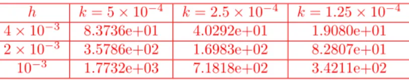
h k= 5×10⁻⁴ k= 2.5×10⁻⁴ k= 1.25×10⁻⁴
4×10⁻³ 8.3736e+01 4.0292e+01 1.9080e+01
2×10⁻³ 3.5786e+02 1.6983e+02 8.2807e+01
10−3 1.7732e+03 7.1818e+02 3.4211e+02
Table 3: Local error when integrating the one-dimensional problem corresponding to data (54) and (55) with Dirichlet boundary conditions with the standard implementation of Lie-Trotter method
Firstly, we consider (1) whereX =C([0,1]) andAis the second-order space derivative. Moreover, we take
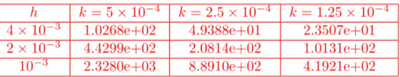
h k= 5×10⁻⁴ k= 2.5×10⁻⁴ k= 1.25×10⁻⁴
4×10⁻³ 1.0268e+02 4.9388e+01 2.3507e+01
2×10⁻³ 4.4299e+02 2.0814e+02 1.0131e+02
10−3 2.3280e+03 8.8910e+02 4.1921e+02
Table 4: Global error when integrating the one-dimensional problem corresponding to data (54) and (55) with Dirichlet boundary conditions with the standard implementation of Lie-Trotter method
h k= 5×10⁻⁴ k= 2.5×10⁻⁴ k= 1.25×10⁻⁴
4×10⁻³ 4.0258e+01 1.9020e+01 8.5800e+00 2×10⁻³ 1.6985e+02 8.2785e+01 4.0137e+01
10−3 7.1836e+02 3.4214e+02 1.6796e+02
Table 5: Local error when integrating the one-dimensional problem corresponding to data (54) and (55) with Dirichlet boundary conditions with the standard implementation of Strang method
and for the Dirichlet boundary conditions,
g0(t) =et, g1(t) =et+1, (55) so that the exact solution of the problem is
u(x, t) =et+x3.
For the space discretization, we take h = 1/(N + 1) and we consider the nodes xj = jh, j = 0, . . . , N + 1. Then, the discrete space is CN, where N
is the number of interior nodes, and the second derivative is approximated by means of the standard second-order difference scheme. Moreover, Ph is
the projection on the interior nodal values, Ah,0 = tridiag(1,−2,1)/h2 and
Chg(t) = [g0(t),0, . . . ,0, g1(t)]T/h2.
Hypothesis (H1a) can be checked to be satisfied by using the logarithmic norm of matrixAh,0, which is given by [14]
µ(Ah,0) = lim
τ→0+
∥I+τ Ah,0∥h−1
τ .
From the logarithmic norm, we obtain the bound
∥etAh,0∥
h≤etµ(Ah,0).
In particular, with the maximum norm (∥u∥∞ = maxi|ui|), which is the one being used in our examples, we have
µ∞(A) = max i
ℜ(aii) +∑ j̸=i
h k= 5×10⁻⁴ k= 2.5×10⁻⁴ k= 1.25×10⁻⁴
4×10⁻³ 4.9213e+01 2.3259e+01 1.0516e+01
2×10⁻³ 2.0805e+02 1.0119e+02 4.9048e+01
10−3 8.8909e+02 4.1915e+02 2.0530e+02
Table 6: Global error when integrating the one-dimensional problem corresponding to data (54) and (55) with Dirichlet boundary conditions with the standard implementation of Strang method
0 0.2 0.4 0.6 0.8 1
10−5
10−4
10−3
10−2
10−1
100
101
102
103
104
X
ERROR AT T=0.2
without avoiding order reduction avoiding order reduction
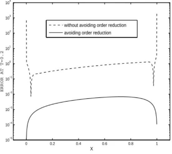
Figure 1: Error at each node at final time when integrating the one-dimensional problem corresponding to data (54) and (55) avoiding and not avoiding order reduction with Lie-Trotter
For the aboveAh,0, it is easily seen thatµ(Ah,0)∞ = 0 and (H1a) holds. On
the other hand, (H1b) can be verified directly from the formula of A−h,10 and it happens that ∥A−h,10∥ ≤ 1
8. Moreover, in this case (H2) is true with Z =
C4([0,1]),∥v∥Z =∥v∥∞+∥vxxxx∥∞ andεh, ηh =O(h2), a discrete maximum principle applies [26] andf satisfies (H3).
Calculatingφj(kAh,0)Chg(t) just corresponds to making a linear
combina-tion of the first and last column of φj(kAh,0), which can be both calculated once and for all at the very beginning for fixed stepsizek. As integrator Ψk, we
have considered the 4th-order classical Runge-Kutta method.
0 0.2 0.4 0.6 0.8 1
10−10
10−8
10−6
10−4
10−2
100
102
104
X
ERROR AT T=0.2
without avoiding order reduction avoiding order reduction
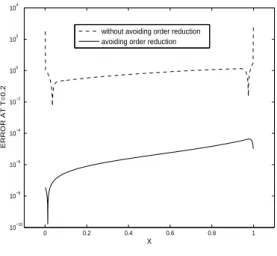
Figure 2: Error at each node at final time when integrating the one-dimensional problem corresponding to data (54) and (55) avoiding and not avoiding order reduction with Strang
the error in space is negligible. (This seems to be the case because decreasing
hdoes not practically change the errors.)
In order to better appreciate the advantage with respect to the standard technique (32), we also show for this problem the results when not avoiding order reduction for both Lie-Trotter and Strang methods for the same values of the parameters hand k. In Tables 3, 4, 5 and 6 we can observe that, not only the order is just 1 for both local and global error, but also the size of errors is unacceptable and even grows when h diminishes. This is not very surprising to us since that has also been observed when exponential Lawson methods integrate time-dependent boundary value problems in the standard way [3]. On the other hand, we also show the error at each node in space after the final time of integration when avoiding and not avoiding order reduction withk= 5×10⁻⁴. Figures 1 and 2 make it obvious that the main difference in
the size of errors comes from the boundary, which is natural taking into account that the technique to avoid order reduction consists of refining the boundary values of the split subproblems.
Let us now consider the same problem as for the previous experiment, but with a Neumann boundary condition at the right boundary. More precisely, the boundary conditions are
u(0, t) = g0(t), (56)
ux(1, t) = g1(t). withg0(t) =et andg1(t) = 3e1+t.
k= 5×10⁻⁴ k= 2.5×10⁻⁴ k= 1.25×10⁻⁴
L∞-local error 2.0286e-04 5.1444e-05 1.2795e-05
Order 1.98 2.01
L∞-global error 3.9872e-02 1.9887e-02 9.9237e-03
Order 1.00 1.00
Table 7: Local and global error when integrating the one-dimensional problem corresponding to data (54), with Dirichlet and Neumann boundary conditions (56), with the suggested modification of Lie-Trotter method
the last row which is [0, . . . ,0,2,−2]/h2now, and
Ch∂u(t) = [g0(t)/h2,0, . . . ,0,2g1(t)/h]T.
Again, hypotheses (H1)-(H3) are satisfied but with ∥A−h,10∥∞ ≤ 1/2, another discrete maximum principle,Z=C4([0,1]) and
∥v∥Z =∥v∥∞+ max(∥vxxx∥∞,∥vxxxx∥∞).
Notice that now, as it is proved by using Taylor expansions, all components of
Ah,0(Rhu−Phu) areO(h2∥uxxxx∥∞) except for the last component which just
decreases as O(h∥uxxx∥∞). Therefore, εh isO(h) andηh is, in principle, also
O(h) for everyu∈C4([0,1]). However,
Rhu−Phu = A−h,10
O(h2∥u
xxxx∥∞)
.. .
O(h2∥u
xxxx∥∞)
0
+A−
1 h,0 0 .. . 0
O(h∥uxxx∥∞)
= O(h2)∥uxxxx∥∞+O(h2)∥uxxx∥∞A−h,10
0 .. . 0 2/h
where, for the last equality, we have used (H1b). Taking now (H2c) into account,
A−h,10[0. . .0 2/h]T is bounded and thereforeηhis in factO(h2).
k= 1×10⁻³ k= 5×10⁻⁴ k= 2.5×10⁻⁴
L∞-local error 2.6922e-05 5.0772e-06 9.1626e-07
Order 2.41 2.47
L∞-global error 1.8549e-04 4.6220e-05 1.0814e-05
Order 2.00 2.10
Table 8: Local and global error when integrating the one-dimensional problem corresponding to data (54), with Dirichlet and Neumann boundary conditions (56), with the suggested modification of Strang method
k= 5×10⁻³ k= 2.5×10⁻³ k= 1.25×10⁻³
L∞-local error 6.1550e-02 1.9049e-02 5.7445e-03
Order 1.69 1.73
L∞-global error 6.1666e-01 2.9307e-01 1.4341e-01
Order 1.07 1.03
Table 9: Local and global error when integrating the two-dimensional problem corresponding to data (57) with the suggested modification of Lie-Trotter method
8.2. Two-dimensional problem
We have also considered the two-dimensional problem in the square Ω = [0,1]×[0,1] when the operatorAis the Laplacian. Moreover, we have considered
u0(x, y) =ex 3+y3
, (x, y)∈Ω, g(t, x, y) =et+x3+y3, (x, y)∈∂Ω, f(t, u, x, y) =u2−et+x3+y3(9(x4+y4) + 6(x+y) +et+x3+y3−1), (57) which hasu(t, x, y) =et+x3+y3 as exact solution.
Firstly, for the discretization of the Laplacian we have considered the stan-dard five-point formula [26]. We notice that, in this case, the discrete space is
CN2
, whereN is the number of interior nodes in each direction, andAh,0 is a tridiagonal block-matrix of dimensionN2. Besides, the matrices in the diagonal are the same and are tridiagonal and the matrices at the subdiagonal and su-perdiagonal are the same and are diagonal. Notice also thatChg(t) would just
have 4N−4 non-vanishing components, which is a number which is negligible compared with N2, the total number of interior nodes. Again, (H1)-(H3) are satisfied for the infinity norm withεh,ηhbeing O(h2) [26].
Tables 9 and 10 show the orders which are observed in time for h= 10−2 in Table 9 and h = 5×10⁻³ in Table 10 when integrating the problem till
timeT = 1 with the suggested modifications of Lie-Trotter and Strang method considering again Ψkas the fourth-order classical Runge-Kutta method. Again,
we see that the local and global order for Lie-Trotter are near 2 and 1 respectively and that the local and global order for Strang are near 2.
k= 1×10⁻² k= 5×10⁻³ k= 2.5×10⁻³
L∞-local error 5.4278e-02 1.6069e-02 4.6066e-03
Order 1.76 1.80
L∞-global error 3.1796e-01 7.7798e-02 2.1844e-02
Order 2.03 1.83
Table 10: Local and global error when integrating the two-dimensional problem corresponding to data (57) with the suggested modification of Strang method
order reduction is avoided in the case of a dimension splitting of the Laplacian operator. We use similar ideas for the discretization of (19) in Lie-Trotter method and that of (26) in Strang method.
More precisely, for the discretization of (19) we firstly consider the problem
z′n(s) = A1zn(s), (58)
zn(0) = un,
∂1zn(s) = ∂(u(tn) +sA1u(tn)),
withA1u=∂xxu, and∂1u={u(0, y) =u(1, y), y∈[0,1]}. Then,
rn′(s) = A2rn(s), (59)
rn(0) = zn(k),
∂rn(s) = ∂2(u(tn) +kA1u(tn) +sA2u(tn)),
where A2u= ∂yyuand and ∂2u = {u(x,0) = u(x,1), x ∈ [0,1]}. Finally, we makevn(k) =rn(k). We apply now the spatial discretization of problems (58)
and (59) and we obtain
Zh,n(k) = ekAh,0,1Uhn+kφ1(kAh,0,1)Ch∂1u(tn) +k2φ2(kAh,0,1)Ch∂1A1u(tn),
Rh,n(k) = ekAh,0,2Zh,n(k) +kφ1(kAh,0,2)Ch∂2(u(tn) +kA1u(tn))
+k2φ2(kAh,0,2)Ch∂2A2u(tn),
where Ah,0,1, Ah,0,2, ∂1, ∂2 are the matrices and the boundaries associated to the spatial discretization ofA1 andA2 respectively.
On the other hand, in order to integrate (26) with Strang method, we firstly consider the problem,
r′n(s) = A1rn(s), (60)
rn(0) = vn
(
k
2
)
,
∂1rn(s) = ∂1
(
u(tn) +
k
2f(tn, u(tn)) +sA1u(tn)
)
then,
ϕ′n(s) = A2ϕn(s), (61)
ϕn(0) = rn
(
k
2
)
,
∂2ϕn(s) = ∂2
(
u(tn) +
k
2f(tn, u(tn)) +
k
2A1u(tn) +sA2u(tn)
)
,
and finally
µ′n(s) = A1µn(s), (62)
µn(0) = ϕn(k),
∂1µn(s) = ∂1
(
u(tn) +
k
2f(tn, u(tn)) +
k
2A1u(tn) +kA2u(tn) +sA1u(tn)
)
,
and we makewn(k) =µn(k2). Considering now the spatial discretization of the
previous three problems, we obtain
Rh,n
(
k
2
)
= ek2Ah,0,1V
h,n+
k
2φ1
(
k
2Ah,0,1
)
Ch∂1
(
u(tn) +
k
2f(tn, u(tn))
)
+k 2
4 φ2
(
k
2Ah,0,1
)
Ch∂1A1u(tn),
Φh,n(k) = ekAh,0,2Rh,n
(
k
2
)
+kφ1(kAh,0,2)Ch∂2
(
u(tn) +
k
2f(tn, u(tn)) +
k
2A1u(tn)
)
+k2φ2(kAh,0,2)Ch∂2A2u(tn),
µh,n
(
k
2
)
= ek2Ah,0,1Φ
h,n(k)
+k 2φ1
(
k
2Ah,0,1
)
Ch∂1
(
u(tn) +
k
2f(tn, u(tn)) +
k
2A1u(tn) +kA2u(tn)
)
+k 2
4 φ2
(
k
2Ah,0,1
)
Ch∂1A1u(tn),
Wh,n = µh,n
(
k
2
)
.
We have considered the standard second order symmetric finite difference scheme for the discretization ofA1 and A2. Notice that this procedure will be especially efficient since now the matricesAh,0,j (j = 1,2) for space
discretiza-tion in one or another direcdiscretiza-tion are block-diagonal matrices after reordering and, moreover, the blocks are tridiagonal. Therefore, multiplying ekAh,0,j or
φl(kAh,0,j) times a vector of sizeN2 just corresponds to N products of a
ma-trix of dimensionN×N times a vector of sizeN. Moreover, many components ofChg(t) will vanish.
k= 5×10⁻³ k= 2.5×10⁻³ k= 1.25×10⁻³
L∞-local error 6.9693e-02 1.9980e-02 5.8275e-03
Order 1.80 1.78
L∞-global error 6.1373e-01 2.9240e-01 1.4325e-01
Order 1.07 1.03
Table 11: Local and global error when integrating the two-dimensional problem corresponding to data (57) with the double splitting of Lie-Trotter method and second-order difference scheme in space
k= 10−2 k= 5×10⁻³ k= 2.5×10⁻³
L∞-local error 6.6803e-02 1.8862e-02 5.2890e-03
Order 1.82 1.83
L∞-global error 3.5131e-01 8.9572e-02 2.3855e-02
Order 1.97 1.91
Table 12: Local and global error when integrating the two-dimensional problem corresponding to data (57) with the double splitting of Strang method and second-order difference scheme in space
9. Conclusions
In this paper a technique is suggested to avoid order reduction when inte-grating reaction-diffusion initial boundary value problems with time-dependent boundary values with Lie-Trotter and Strang splitting methods. We have made a through analysis for the error both in space and time and we have considered not only Dirichlet, but also Neumann and Robin boundary conditions. More precisely, we have specified how to calculate either exactly or approximately the required boundary values for the split subproblems for the different types of boundary conditions and we have even inserted into the analysis the possible error coming from this approximation.
We have numerically verified the great improvement in accuracy with respect to the standard way of implementing the methods which, as it is natural, is more obvious near the boundary.
The results in this paper have already been extended in the set of nonlinear problems to exponential Lawson methods [11] and some research is also being done on its extension to other Runge-Kutta type exponential methods [9].
Acknowledgements
References
[1] I. Alonso–Mallo, B. Cano and N. Reguera, Avoiding order reduc-tion when integrating linear initial boundary value problems with exponential splitting methods,IMA J. Numer. Anal.,38(2018), 1294-1323.
[2] I. Alonso–Mallo, B. Cano and N. Reguera, Analysis of order re-duction when integrating linear initial boundary value problems with Lawson methods, Appl. Numer. Math.,118(2017), 64-74.
[3] I. Alonso–Mallo, B. Cano and N. Reguera,Avoiding order reduction when integrating linear initial boundary value problems with Lawson methods, IMA J. Numer. Anal., 37(2017), 2091-2119.
[4] I. Alonso–Mallo, B. Cano and N. Reguera, Looking for efficiency
when avoiding order reduction in nonlinear problems with Strang splitting, http://arxiv.org/abs/1709.09849.
[5] I. Alonso–Mallo, B. Cano and N. Reguera,Comparison of efficiency among different techniques to avoid order reduction with Strang splitting, sub-mitted for publication.
[6] I. Alonso–Mallo and C. Palencia,On the convolutions operators aris-ing in the study of abstract initial boundary value problems, Proc. Royal Soc. Edinburgh.126A(1996), 515–539.
[7] W. Arendt,Semigroups and evolution equations: functional calculus, reg-ularity and kernel estimates. Evolutionary equations. Vol. I, 1–85, Handb. Differ. Equ., North-Holland, Amsterdam, 2004.
[8] W. Arendt,Resolvent positive operators and inhomogeneous boundary con-ditions, Ann. Scuola Norm. Sup. Pisa Cl Sci. (4), 29 (2000), 639-670. [9] B. Cano and M. J. Moreta,How to avoid order reduction when
Runge-Kutta exponential methods integrate reaction-diffusion initial boundary value problems, in preparation.
[10] B. Cano and N. Reguera, Avoiding order reduction when integrating nonlinear Schr¨odinger equation with Strang method, J. Comp. Appl. Math., 316 (2017), 86–99.
[11] B. Cano and N. Reguera,How to avoid order reduction when Lawson methods integrate reaction-diffusion initial boundary value problems, submit-ted for publication.
[12] H. Cartan,Calcul diff´erentiel. Hermann, Paris, 1967.
[13] J. Connors, J.W. Banks, J.A. Hittinger, and C.S. Woodward,
[14] G. Dahlquist, Stability and error bounds in the numerical integration of ordinary differential equations. Trans. Royal Inst. of Technology. No. 130, 1959. Thesis 1958.
[15] L. Einkemmer and A. Ostermann, Overcoming order reduction in
diffusion-reaction splitting. Part 1: Dirichlet boundary conditions, SIAM J. Sci. Comput.37(3) (2015), A1577–A1592.
[16] L. Einkemmer and A. Ostermann, Overcoming order reduction in
diffusion-reaction splitting. Part 2: Oblique boundary conditions, SIAM J. Sci. Comput.38(2016) A3471-A3757.
[17] E. Faou, A. Ostermann and K. Schratz,Analysis of exponential split-ting methods for inhomogeneous parabolic equations, IMA J. Numer. Anal.35
(1) (2015), 161–178.
[18] T. Gockler and V. Grimm,Convergence analysis of an extended Krylov subspace method for the approximation of operator functions in exponential integrators, SIAM J. Numer. Anal.51(4) (2013), 2189–2213.
[19] E. Hansen, F. Kramer, A. Ostermann,A second-order positivity pre-serving scheme for semilinear parabolic problems, Appl. Numer. Math. 62 (2012), no. 10, 1428–1435.
[20] D. Henry,Geometric Theory of Demilinear Parabolic Problems, Lectures Notes in Mathematics, 840, Springer verlag, New York, 1981.
[21] M. Hochbruck and A. Ostermann,Exponential Runge-Kutta methods for parabolic problems, Appl. Numer. Math.53(2005), no. 2-4, 323–339. [22] M. Hochbruck and A. Ostermann,Exponential integrators, Acta
Nu-merica (2010) 209-286.
[23] R. J. LeVeque and J. Oliger, Numerical methods based on additive splittings for hyperbolic partial differential equations, Math. Comp. 40 (1983), no. 162, 469–497.
[24] C. Palencia and I. Alonso–Mallo, Abstract initial-boundary value problems, Proceedings of the Royal Society of Edinbourgh. Section A- Math-ematics. 124, (1994) 879 - 908.
[25] A. Pazy,Semigroups of Linear Operators and Applications to Partial Dif-ferential Equations, Series: Applied Mathematical Sciences, Vol. 44, Springer, New York, Berlin, Heidelberg, Tokyo, 1983.