1
UNIVERSIDAD AUTÓNOMA DE NUEVO LEÓN
FACULTAD DE CIENCIAS FÍSICO-MATEMÁTICAS
Hypothesis test for changes in variance using a statistic based in P-values in a time series of normal independent observations.
Por
Samuel Uriel Armendáriz Hernández
Como requisito parcial para obtener el grado de:
Maestría en Ciencias con Orientación en Matemáticas
1 UNIVERSIDAD AUTÓNOMA DE NUEVO LEÓN
FACULTAD DE CIENCIAS FÍSICO-MATEMÁTICAS
Hypothesis test for changes in variance using a statistic based in P-values in a time series of normal independent observations.
Por
Samuel Uriel Armendáriz Hernández
Como requisito parcial para obtener el grado de:
MAESTRÍA EN CIENCIAS CON ORIENTACIÓN EN MATEMÁTICAS.
3 of normal independent observations.
Por
Samuel Uriel Armendáriz Hernández
Como requisito parcial para obtener el grado:
MAESTRO EN CIENCIAS CON ORIENTACIÓN EN MATEMÁTICAS.
Miembros del comité:
______________________________________________________ Dr. Alvaro Eduardo Cordero Franco
Asesor
_________________________________ Dr. Víctor Gustavo Tercero Gómez
Co-asesor
___________________________________ Dr. Francisco Javier Almaguer Martinez
iv Content
Acknowledgements ... vii
Figure list ... ix
Table list ... x
Abstract ... 1
CHAPTER 1. - INTRODUCTION ... 2
1.1. Introduction ... 2
1.2. History and background of change point analysis for shift in variance ... 4
1.3. Problem Statement ... 5
1.4. Research questions ... 5
1.5. Research hypotheses ... 6
1.6. Objective ... 6
1.7 Justification ... 7
1.7.1 Scientific justification ... 7
1.7.2 Practical justification ... 7
1.8 Scope and limits ... 8
CHAPTER 2. LITERATURE REVIEW ... 9
2.1 Change point analysis. ... 11
2.1.1 Classical Analysis ... 11
2.1.2 Non parametric analysis. ... 11
2.2 Tests for shift in variance. ... 12
2.3 GLR control charts ... 12
v
CHAPTER 3. THEORETICAL FRAMEWORK ... 14
3.1 Hypothesis tests... 14
3.2 P-values ... 15
3.3 The F distribution ... 16
3.3.1 Definition ... 16
3.3.2 F test ... 16
3.4 Regression Analysis ... 17
3.4.1 Linear Simple Regression ... 17
3.4.2 Regression with transformed variables. ... 18
CHAPTER 4. PROPOSED MODEL ... 20
4.1 Model ... 20
4.2 Quantile estimation ... 22
4.3 Reciprocal regression. ... 23
4.4 Power of the test ... 28
4.5 Comparison with Che ’s Test 997 . ... 31
4.6. – Numerical Example ... 33
CONCLUSIONS AND FUTURE WORK ... 35
Conclusions ... 35
Future work ... 36
REFERENCES ... 38
APPENDIX ... 41
A.1 Matlab codes ... 41
A.1.1 Quantile estimation ... 41
vi
A.1.3 Comparison for decreasing variance ... 43
A.1.4 Comparison for increasing variance ... 45
A 1.5 Numerical Example ... 47
A.2 All the Quantiles ... 48
Appendix 3. Plots. ... 60
A.3.1 Power of Samuel´s test. ... 60
vii Acknowledgements
In the first place, I want to comply the commandment to remember Hashem who gives me
the power to get wealth (Deuteronomy 8:18). He is the cause of all the causes. Everything,
the good and the evil come from him. His partners that helped me to achieve this goal are:
My parents: Juan and Teresa. You are the light of my life, you gave me a family, you feed
me, you educated me and in return I made you cry, I lied to you, I stole your sleep hours
and you resisted all this behavior only because you love me. Only remember that the day
was created the first half as darkness and the second half as light. I think my life was
designed in the same way. Therefore as you did ’t fo get who I was while I was living my
dark period I o ’t fo get ou a d my siblings now when all this sacrifice fructifies.
My siblings: Jaziz, Juan, a d Jael. I did ’t spe d enough time with you since I enrolled high
school, looking for my needs while ig o i g ou s. I do ’t know you as well as your friends.
Sometimes I feel like a stranger when I talk to you. The good point of this is the fact that
our personalities are antipodal because we move in very different social networks with
different people. This will allow us to sha e ou pa e ts’ tea hi gs a d alues ith o e
people. I hope with all my heart to see your professional and personal success.
Doctor Eduardo Cordero and Doctor Victor Tercero, the honored place for the people
directly involved in my professional development is for you. You are the only ones, after my
parents that kept the faith after many fails. Your confidence in me never decreased. You
gave me a topic to work for my thesis, you gave me recommendations when required. You
included me in your activities and projects despite you knew the probability that I would
not do my part. You connected me with people. You paid the bill many times, and you
became a figure to follow. Therefore, this is achieve is for you.
Doctor Javier Almaguer, thank you for accept the invitation to be one of my evaluators and
for all the support offered during my studies.
Pana, Cristina and Tenorio, you supported me with comments and gave me permission to
viii My classmates Diego and Armando thanks for teaching me the meaning of team.
Doctors Fernando Camacho and Aracelia Alcorta, you gave me the opportunity to enroll
this program and the opportunity to conclude it. It was worth it.
Julian Galvan and Esther Grimaldo, my bosses. You gave me a job opportunity and all the
permissions I needed to conclude my Thesis.
CONACYT thanks for your support and commitment to science in Mexico.
Gabriela Medellin thank you all the paperwork with the scholarship and the corresponding
renovation.
My wife, offspring, grandchildren and all descendants ad infinitum all my things are yours
and all my achievements are yours e e if I do ’t k o you yet. I am currently working to
be the best version of me, to give you the best life and education. I will be waiting for the
ix Figure list
Figure 1: Graphs of intrinsically linear functions in Table 2 ... 18
Figure 2: Bottom quantiles ... 22
Figure 3: Top quantiles ... 23
Figure 4: Quantiles after reciprocal transformation ... 24
Figure 5: Hawkins (blue) versus Reciprocal (red) regression error. ... 25
Figure 6: Hawkins fitted curve (green) vs. Reciprocal fitted curve (red). ... 26
x Table list
Table 1: Literature review ... 10
Table 2: the most useful intrinsically linear functions ... 18
Table 3: Correlation coefficients after reciprocal transformation. ... 24
Table 4: Quantile equations. ... 26
Table 5: Quantile table for T<51 ... 28
Table 6: Power of Proposed test for α=0.05 ... 29
Table 7: Power of Proposed test for α=0.95 ... 30
Table 8: Values of ... 31
1 Abstract
The present work proposes a Hypothesis Test to detect a shift in the variance of a series of
independent normal observations using a statistic based on the p-values of the F
distribution. Since the probability distribution function of this statistic is intractable,
critical values were we estimated numerically through extensive simulation. A
regression approach was used to simplify the quantile evaluation and extrapolation.
The power of the test was simulated using Monte Carlo simulation, and the results
were compared with the Chen test (1997) to prove its efficiency. Time series
analysts might find the test useful to address homoscedasticity studies were at
2
CHAPTER 1. - INTRODUCTION
1.1.Introduction
There are not ideal processes, every process presents variability. Quality engineers define
quality is defined as the reduction of variability. Due to this, it is necessary to monitor the
variability of a process. In some industries, the shift in variance is very important. For
instance, a pharmaceutical process cannot exceed some critical amount of an active
substance and reduce drastically in the next batch. Maybe the mean will be under control
but variability might trigger fatal or ineffective cases. Nevertheless, most of the efforts to
detect change points have been developed to monitor change points for a shift in mean. In
the literature reviewed in Chapter two, only 7 articles regarding change-points in variance
were found, 5 of them were written after 2012.
In summary:
There is a need in some industries to keep their processes with constant variance.
There are few tools available today to attach these requirements from a
change-point approach.
The number of researchers developing tools to detect shifts in variance is increasing
in the last years. This shows the fact that the statistic community is interested in
this field.
Cordero (2012) and Tercero (2012) have used p-values of chi-squared and F
distributions respectively to create control-charts for this purpose.
Concerning a retrospective analysis, hypothesis tests based on p-values of a shift in
variance have not been developed yet.
Due to this, in this research a statistic based on the p-values of iterative F-tests for
detecting shifts in variance is proposed.
Statistical Control Process (SPC) studies how to monitor the process and determine
3 of 2 phases: Phase 1: estimation and Phase 2: detection. Shewhart is considered the father
of SPC. I 93 he pu lished his ook alled E o o i Co t ol of Qualit of
Manufa tu ed he e he established the philosophy and designed the first basic statistical
tool to monitor the process, the first control charts, where he included a dispersion graph
displaying the data, the mean and the upper and lower limit controls. This control chart is
currently used by most of the practitioners in the manufacturing as can be read in Western
Electric- A Brief history:
By the turn of the century, Western Electric had trained individuals as inspectors to assure
specification and quality standards, in order to avoid sending bad products to the customer.
In the 1920's, Western Electric's Dr. Walter Shewhart took manufacturing quality to the next
level--employing statistical techniques to control processes to minimize defective output.
When Dr. Shewhart joined the Inspection Engineering Department at Hawthorne in 1918,
industrial quality was limited to inspecting finished products and removing defective items.
That all changed in May 1924. Dr. Shewhart's boss, George Edwards, recalled: "Dr.
Shewhart prepared a little memorandum only about a page in length. About a third of that
page was given over to a simple diagram which we would all recognize today as a
schematic control chart. That diagram, and the short text which preceded and followed it,
set forth all of the essential principles and considerations which are involved in what we
know today as process quality control." Mr. Edwards had observed the birth of the modem
scientific study of process control. That same year, Dr. Shewhart created the first statistical
control charts of manufacturing processes, which involved statistical sampling procedures.
Shewhart published his findings in a 1931 book, Economic Control of Quality of
Manufactured Product .
The Change-point analysis is a branch of SPC which deals with the detection and estimation
of changes in series of observations; this is, given a sequence of observations of the
variables with distribution
4 Find ; the initial moment when a change occurs. In this research, we propose a test for
detecting changes in variance in a sequence of independent normal observations.
1.2.History and background of change point analysis for shift in variance
In 1994 Carla Inclan and George Tiao used cumulative sums of squares to search for change
points systematically at different pieces of the series. This approach was based on a
centered version of the cumulative sum of squares following an algorithm to find multiple
change points in an iterative way.
In 1997 Jie Chen and Arjun K. Gupta designed a hypothesis test for shift in variance using
Schwarz Information criterion and Maximum Likelihood function of the model. They
presented it again in 2001. This test will be deeply studied in Chapter 5.
In 2005 Hawkins and Zamba extended the work of Hawkins et al. (2003) to develop a
control chart for shift in variance with the change point methodology and based in the
Ge e alized Likelihood Ratio Test ith the Ba tlett’s o e tio adapted fo its se ue tial
use.
Tercero et al. (2012) developed a generalized LR control chart capable of detecting shifts in
variance and estimate the initial moment of this change at the same time using the p-value
function of the F statistic. These p-values are used to construct the Hypothesis Test of the
present work.
Cordero et al. (2012) presented a generalized likelihood control chart by using the p-value
of the Chi-Squared statistic capable of detecting shifts in variance and estimate the initial
moment of the change at the same time.
Garza (2013) developed estimators for shift in mean, variance or both and MLE for time
series with multiple change points using a construction Heuristic and Genetic Algorithm to
assess the problem of finding MLES, which is a NP optimization problem.
Finally, Villanueva (2013) created a non-parametric control chart based in the model
5 1.3.Problem Statement
Let be a set of independent observations following the next distribution:
{
In this research a hypothesis based on F test is designed to determine if there is a shift in
the variance will be developed. The null hypothesis for this test is and the
alternative hypothesis is .
Chapter 1 presents the proposal of this research; chapter 2 presents the literature review
in change point and SPC. Chapter 3 contains the theoretical framework necessary to
develop this research. Readers with a strong statistical background can omit it. Chapter 4
presents the proposed test, an evaluation of the power of this test and a comparison with
Che ’s test 997). After this, a Chapter with conclusions and ideas for future work is
added. Finally, the appendix shows the Matlab code, a complete table of all the critical
values estimated and all the stages simulated for power of the test analysis for proposed
test a d Che ’s test (1997).
1.4.Research questions
As was mentioned in section 1.1, in this research a test to detect changes in variance in a
normal sequence of observations based on the P-values of the F test is proposed. To
analyze the efficiency of this test the following steps are required:
Calculate the power of the test proposed with simulated data to validate if really
detects a shift i a ia e he it e ists a d does ’t dete t a shift i a ia e he
it does ’t e ist.
If the test works correctly, it must be compared with another test under the same
conditions to decide in the first place the test with the biggest accuracy and
secondly some advantages and disadvantages of both tests.
6 Question 1. Is the proposed test an unbiased test?
Question 2. How is the power of the proposed test compared to the power of another
similar test?
1.5.Research hypotheses
According to questions posed in section 1.4, the correspondent hypotheses are.
Hypothesis 1. The proposed test is an unbiased test, this is, and the probability of
committing a type I error is less than the significance level and the probability of
committing a type 2 error is at least that of the significance level.
Hypothesis 2. The power of this test is bigger than at least, the power of another test in
literature, this is; the proposed test rejects the null hypothesis more times when it is false
while both tests are performed under the same conditions.
1.6.Objective
The main objective of the present research is to develop a new unbiased test for changes in
variance based in the p-values of F distribution. To achieve this goal, series of normally
distributed data with constant mean and variance must be simulated. Let be the size of
one series and be a set of independent normal observations. For each
we calculate the p value of F test to detect if there is change in variance before and after . We take the smallest p-value, which indicates the point where the
probability to have a decrement in variance is maximum. Analogously the biggest p-value
indicates the point with maximum probability to have an increment in variance. After
replicating this process several times, we will choose specific quantiles for each p-value
7 1.7Justification
Applied mathematicians solve real life problems that generate value to society using math.
Therefore a strict analysis of the potential impact and contributions to science and industry
generated with this research is necessary. The present section contains such analysis.
1.7.1 Scientific justification
This research aims to cover the following requirements in science:
The problem of detecting a shift in variance has received less attention than the
detection of changes in the mean. This could be because the power of this kind of
tests is very poor.
The development of this test can be used in a control chart for an online monitoring
of the variance of the process.
Some of the methods that detect shifts in mean assume equality in variances.
Therefore, this hypothesis test can be used as a previous step for those methods.
1.7.2 Practical justification
Montgomery (2008), states that quality is inversely proportional to the variability. This is
why industry must maintain variance in the least possible level. The first step to attach this
goal is to identify the steps of the process presenting uncontrolled variance. After this,
decisions must be taken and strategies must be designed according to the situation.
This research will provide a new tool that will help industry to automatize the first step
using the state of the art in Change Point Analysis.
Examples of industries whose requirements of variance must be extremely exigent are:
Pharmaceutical industry.
Biometrical security systems.
Jewelry creation.
Fire alarms.
8 1.8 Scope and limits
9
CHAPTER 2. LITERATURE REVIEW
In this section a complete literature review is presented. In order to introduce the reader
gradually, this section begins presenting contributions to Change Point analysis in general
and finalizing in those works closely related with the hypothesis test developed here.
Thus the subsections of this chapter are:
A general overview of change point analysis (2.1)
Tests for shift in variance (2.2)
GLR control charts (2.3)
P value based tests and charts (2.4)
Table 1 presents all the sources chronologically with a brief description to ease the search
of a specific paper. This table does not include textbooks consulted for section 3. These
books are listed in that section.
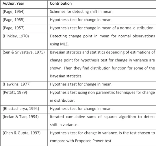
Author, Year Contribution
(Page, 1954) Schemes for detecting shift in mean.
(Page, 1955) Hypothesis test for change in mean.
(Page, 1957) Hypothesis test for change in mean of a normal distribution.
(Hinkley, 1970) Detecting change point in mean for normal observations
using MLE.
(Sen & Srivastava, 1975) Bayesian statistics and statistics depending of estimations of
change point for hypothesis test for change in variance are
shown. Then they find distribution function for some of the
Bayesian statistics.
(Hawkins, 1977) Hypothesis test for change in mean.
(Pettitt, 1979) Hypothesis test using non parametric techniques for change
in distribution.
(Bhattacharya, 1994) Hypothesis test for change in mean.
(Inclan & Tiao, 1994) Iterated cumulative sums of squares algorithm to detect
shift in variance.
(Chen & Gupta, 1997) Hypothesis test for change in variance. Is the test chosen to
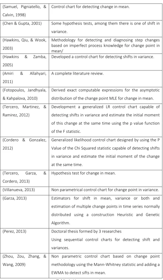
10 (Samuel, Pigniatello, &
Calvin, 1998)
Control chart for detecting change in mean.
(Chen & Gupta, 2001) Some hypothesis tests, among them there is one of shift in
variance.
(Hawkins, Qiu, & Wook,
2003)
Methodology for detecting and diagnosing step changes based on imperfect process knowledge for change point in mean/
(Hawkins & Zamba,
2005)
Developed a control chart for detecting shifts in variance.
(Amiri & Allahyari,
2011)
A complete literature review.
(Fotopoulos, Jandhyala,
& Kahpalova, 2010)
Derived exact computable expressions for the asymptotic
distribution of the change point MLE for change in mean.
(Tercero, Martinez, &
Ramirez, 2012)
Development a generalized LR control chart capable of
detecting shifts in variance and estimate the initial moment
of this change at the same time using the p value function
of the F statistic.
(Cordero & Gonzalez,
2012)
Generalized likelihood control chart designed by using the P
Value of the Chi Squared statistic capable of detecting shifts
in variance and estimate the initial moment of the change
at the same time.
(Tercero, Garza, &
Cordero, 2013)
Hypothesis test for change in mean.
(Villanueva, 2013) Non parametrical control chart for change point in variance.
(Garza, 2013) Estimators for shift in mean, variance or both and
estimation of multiple change points in time series normally
distributed using a construction Heuristic and Genetic
Algorithm.
(Perez, 2013) Doctoral thesis formed by 3 researches
Using sequential control charts for detecting shift and
variances.
(Zhou, Zou, Zhang, &
Wang, 2009)
Non parametric control chart based on change point
methodology using the Mann-Whitney statistic and adding a
EWMA to detect sifts in mean.
11 2.1 Change point analysis.
To analyze CPA literature the main focuses must be clearly defined
Classical analysis of Change point problem implies the use of descriptive and
inferential statistical tools to realize change point estimations. This approach
considers known the data distribution although its parameters maybe unknown.
Non parametric analysis supposes that function of distribution cannot be defined a
prior. This adds complexity to the problem of detect if the process is under
statistical control because parametric statistical inference methods are not valid
here.
2.1.1 Classical Analysis
One of the pioneers in this area is Page. In 1954 he presented a control chart based in the
cumulated sum of observations (CUSUM), reporting bigger sensibility to small and
sustained changes than Shewhart control Charts. In the next years he continued publishing
in this area.
In 1970 Hinkley founds the basis for using MLE to estimate the change point, which implies
the use of derivatives to determine maximum and minimum values.
In 1998 Samuel, Pignatiello and Calvin presented an alternative for change point detection
from the use of MLE for shift in mean once the control chart detects that process is out of
statistical control.
2.1.2 Non parametric analysis.
Again Page is a pioneer in this field proposing a test based in the redefinition of a variable
and binomial distribution in 1955.
Bhattacharya began to develop non parametric procedures in the way known today using
Wil o o ’s sig al test. Pettit 979 o ked ith this app oa h fo Be oulli a d Bi o ial
12 2.2 Tests for shift in variance.
In 1997 Jie Chen and Arjun K. Gupta designed a hypothesis test for shift in variance using
Schwarz Information criterion and Maximum Likelihood function of the model.
Performance of this test is very similar to CUSUM based tests.
Perez (2013) published used a self-start control chart and MLE for Sequential detection and
estimation of sustained shifts in mean and variance of time series for normally distributed
observations.
On the other hand Garza (2013) used a construction Heuristic and Genetic Algorithm for
designing estimators for shift in mean, variance or both and estimation of multiple change
points in normally distributed time series in order to assess the problem of finding MLES, a
NP optimization problem.
2.3 GLR control charts
Hawkins and Zamba (2005) developed a GLR test ased o Ba tlett’s test for mean and
variance of normally distributed data using only one test for all cases: change only in mean,
only in variance or both parameters for sequential use.
Zou, Zou, Zhang & Wang (2009) developed a non-parametric control chart based in
Hawkins (2003) change point methodology using the Mann-Whitney statistic and adding a
EWMA to detect sifts in mean.
Villanueva (2013) used Hawkins methodology (2005) with a non-parametric statistic to
create a control chart for shit in variance and finding correspondent control limits.
2.4 P-value based tests and charts.
Cordero (2012) et al. developed a generalized control chart based in the P value of chi
squared test with the objective of detecting and estimating shifts in variance in normal
process in phase II based on the GLR procedure. This GLR chart for variance in a normal
process takes into account the knowledge of the process resulting in a chart with better
13 Meanwhile Tercero et al. (2012) created a Generalized Likelihood Ratio chart capable of
detecting shifts in variance and estimate the initial moment of this change at the same
time. They used a moving window instead an ever growing set of observations and the P
value for F test was taken to build an estimator and a statistic to be controlled. This method
works in Phase I of SPC.
After observing the evolution of CPA and SPC the next step is to design a Hypothesis test
based on P-values of F distribution. If the performance of this test is the expected, many
14
CHAPTER 3. THEORETICAL FRAMEWORK
The Hypothesis test proposed in the present work is based on the P-values of the F
distribution. In order to make this contribution accessible to most of the readers the
present Chapter is included. This chapter covers the following themes:
Hypothesis tests (3.1). This concept is the heart of the research because we are
creating a new hypothesis test.
P-values (3.2). The hypothesis test is based on P-values.
The F distribution (3.3). The P-values used in this research come from F distribution.
Future researches probably will need P-values from other distributions.
Regression Analysis (3.4). Regression was need to fit a curve over obtained
quantiles.
Readers with strong statistical basis can omit this section without problem.
3.1 Hypothesis tests
A statistical hypothesis is a conjecture about one or more random variables. For instance, if
a smartphone manufacturing company wants to choose if the time of discharge of the
battery when the smartphone is not used is at least 24 hours, they have to prove the
hypothesis where is the parameter of the exponential distribution.
To achieve this we need to define a rules set to decide if we accept or reject our
hypothesis. This set of rules is called the Hypothesis Test. We will call to the hypothesis
to be proved and to the alternate hypothesis (when is not accepted).
When testing the hypothesis we can make 2 types of errors. The rejection of when is
true is called the type 1 error. The probability of committing a type 1 error is denoted
with . On the other hand if we accept when is false we are making a type 2 error. The
15 The rejection region of is called the critical region of the test. The probability of obtain a
value of the statistic inside this region when is true is called the size of the critical region,
this is . This probability is also called the significance level.
A good hypothesis test has small and . If we maintain the size of the sample constant,
the type 1 error decreases when type 2 error increases and vice versa. The only way to
reduce both errors is increasing the size of the sample.
The power of the test is defined by the probability of rejecting inside and outside the
critical region, this is:
{
This function is useful to compare two tests. A test is better than other wen it has the
smallest probability of committing a type 1 error
3.2 P-values
The p value is a function of the observed sample results (a statistic) that is used for testing
a statistical hypothesis. If the P value is equal or smaller than the significance level, it
suggests that the observed data are inconsistent with the assumption that the null
hypothesis is true and thus that hypothesis must be rejected. When p value is calculated
correctly, such a test is guaranteed to control the type 1 error rate to be no greater than .
To summarize, the p- value is the extreme value where we can accept the null hypothesis.
If the statistic obtains a value less than the P-value, is very probable that you are outside of
the a epta e egio . I te s of this esea h, getti g a statisti ’s alue less tha the P
-value is very probable that there is a change in variance. If we take the least p -value, we are
16 3.3 The F distribution
3.3.1 Definition
The F distribution plays a very important role in the sampling of normal data. This
distribution is named in honor of Sir Ronald A. Fisher, one of the most prominent
statisticians of the past century. F distribution is usually defined in terms of distribution.
If and are random chi- squared variables with independent distributions and ,
degrees of freedom respectively then
Is a random variable with F Distribution, this is, a random variable whose density is given
by:
For and in any other case.
This result is applied in situations where we are interested in comparing the variance of 2
populations. For instance the problem of estimating or validate if .
3.3.2 F test
An F Test is a statistical test in which the test statistic has an F distribution under the null
hypothesis.
Given random samples of normally distributed independent variables of sizes and
and variances the critical region to prove the null hypothesis versus the
alternative are:
17
If .
3.4 Regression Analysis
The distribution of the test statistic is unknown yet. However, quantiles can be estimated
through simulations, where curves can be fitted as a function of the sample size. To fit a
curve is useful for two reasons: first, is more practical to work with a simple equation than
using a huge table. In the other hand, an equation allows users to calculate values of the
test statistic for sizes whose computation time make them unpractical to calculate in
production line.
The chosen tool for this purpose is regression analysis; a statistical process for estimating
relationship among variables.
In the present work we will study the behavior of a dependent variable and an independent
variable.
3.4.1 Linear Simple Regression
The simplest case is the Simple Linear Regression. Here we have a relationship of the form
Where is a random variable and is just another observable variable.
The difference between ̂ and the actual observation is called the error .
Our objective when fitting a curve is to minimize the sum of errors. But when we have both
positive and negative errors they can eliminate between them and small sum or mean of
errors is not always synonym of the best curve fitted. Instead of this, Statisticians minimize
the sum of square of the errors (SSE), since this is always a nonzero quantity, offering the
same advantages that variance add to mean. Due to this the method for calculating slope
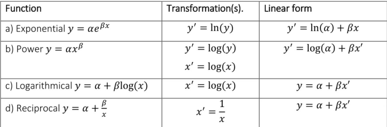
18 3.4.2 Regression with transformed variables.
A function that relates with is intrinsically linear if after transforming one or both
variables they have a linear relationship. The next table resume the most useful intrinsically
linear functions. Whe appea s log ou a use loga ith to the ase o .
Function Transformation(s). Linear form
a) Exponential
b) Power
c) Logarithmical
d) Reciprocal
Table 2: the most useful intrinsically linear functions
The next image is taken from De o e’s book and will help us to select the most appropriate
transformation for each model.
Figure 1: Graphs of intrinsically linear functions in Table 2
In this section the statistical background necessary to develop this research was presented.
The information provided in this section is an introductory description of key topics. For
19
Estadísti a ate áti a o apli a io es (Freund & Miller, 1999).
P o a ilidad estadísti a pa a i ge ie ía ie ias (Devore, 2008).
20
CHAPTER 4. PROPOSED MODEL
This section describes the proposed test for changes in variance. To attach this goal with
the proper order this research is structured in the following way.
Model (4.1). The model is formally enunciated, the methodology is extensively
described and the S statistic is defined.
Quantile estimation (4.2). Most important quantiles are numerically calculated for
sample sizes of at most 500.
Regression (4.3). A curve fitting method is selected and calculated in order to
predict values of S statistic for sample sizes bigger than 500.
Power of the test (4.4). The performance of the test is calculated under some stages
and results are described.
Comparison with Che ’s test (4.5). Finally, the performance of this test is compared
to the performance pf the test presented by Chen & Gupta (1997).
In order to avoid making this work too extensive, in this section are presented only the
most representative results. To consult the complete results of the simulations and the
MATLAB ® codes please consult the appendix.
4.1 Model
Let be a set of independent observations following the next distribution:
{
Let be and and suppose that , the change-point is unknown.
For each we estimate the mean and variance prior and after the change
point:
21
̂ ∑
̂ ∑ ̂
̂ ∑ ̂
And the statistic is computed as follows for each .
̂ ̂
This statistic follows a distribution where and .
The P-value for this test is obtained by:
We reject with type 1 error equal to if
For left tail. ( ) For right tail.
Where is the quantile of the p-value distribution for size= and significance level .
To guarantee this type 1 error we must find the values of under such that
For left tail. ( ) For right tail.
Given that the distribution of and are intractable, it is impossible to calculate the values of . Therefore thes values will be obtained in the next section
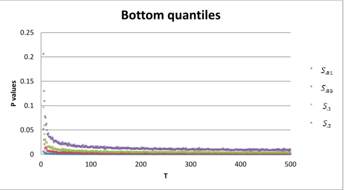
22 4.2 Quantile estimation
The exact distribution of the statistic based on the p-values is unknown yet, and then is
needed to calculate some quantiles of this distribution numerically in order to use them as
critical values of the statistic.
For each we calculate the statistic as shown in the section 4.1 and save the
results in the vector . Then this vector is sorted in increasing order. We take the biggest
and the smallest element of . This process is repeated 1000 times and saved in two
vectors: for the biggest p values and with the smallest. These vectors are
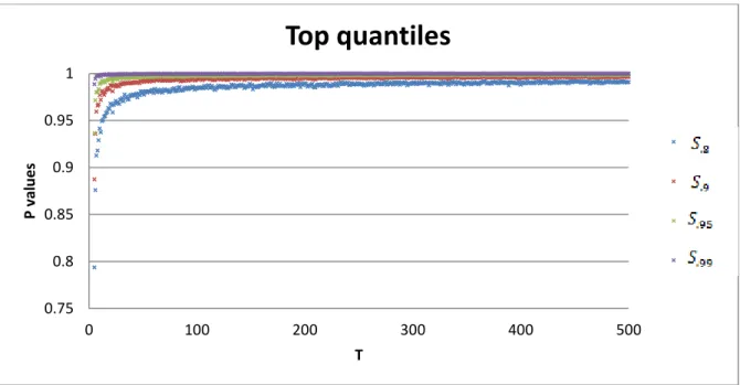
sorted again. Finally we take the elements , , , , , ,
and , which represent the Quantiles , , , , , , and . These elements were saved in an excel file. The time of execution of this program was of
over 2 weeks. Matlab code used to implement this algorithm can be consulted in the
Appendix 1 and the complete table of all Quantiles can be consulted in the Appendix 2.
Figure 2 and figure 3 display plots of the data horizontal axis represent the size of the
sample and vertical axis represents the P-value.
Figure 2: Bottom quantiles of statistic based on p-values
0 0.05 0.1 0.15 0.2 0.25
0 100 200 300 400 500
23 Figure 3: Top quantiles of statistic based on p-values
The exact distribution of the quantiles is unknown yet. As was mentioned in section 3.4, is
necessary to fit a curve for two reasons: first, is more practical to work with a simple
equation than using a huge table and having an equation allows users to calculate values of
the test statistic for sizes whose computation time make them unpractical to calculate in
production line.
According to the data visualization in figure 3 and 4 and comparing with figure 1 a
reciprocal transformation is suggested.
4.3 Reciprocal regression.
The transformation consists in make and . If this transformation is the most
appropriate then and will be linearly related and both regressions will have the same
parameters, this is, if . After doing this transformation we
obtain the following correlation coefficients (Table 3):
Quantile 10/1000 0.917876215
Quantile 50/1000 0.90538046
Quantile 100/1000 0.938721886 0.75 0.8 0.85 0.9 0.95 1
0 100 200 300 400 500
24 Quantile 200/1000 0.958885348
Quantile 801/1000 -0.960948301
Quantile 901/1000 -0.925966965
Quantile 951/1000 -0.884818859
Quantile 991/1000 -0.860428257
Table 3: Correlation coefficients after reciprocal transformation.
Figure 4 displays the data after the transformation.
Figure 4: Quantiles after reciprocal transformation
An exhaustive analysis was required to ensure the accuracy of this regression technique.
For this purpose we compared this method with the proposed by Hawkins (2005) and used
by Villanueva (2005).
1. Give initial values to the next equation
√ where 0.05 is the significance level.
2. Calculate the sum of the square errors.
3. Using the SOLVER included in the MS Excel software we obtain the minimum value
of the sum of the square errors by varying the values of the parameters of the
25 The reciprocal regression had a better performance with smaller sum of squares of errors,
s alle a i u a solute e o a d the e o s did ’t show tendency as in the Hawkins
equation. For proposed test obtained sum of square errors of against
obtained by Hawkins regression. Maximum absolute error for proposed test was and for Hawkins regression was . Figure 5 represents the
errors of the regression and figure 6 contains the plots of both curves. Observe that
reciprocal equation gets stable after T=50.
Figure 5: Hawkins (blue) versus Reciprocal (red) regression error.
-0.12 -0.1 -0.08 -0.06 -0.04 -0.02 0 0.02
26 Figure 6: Hawkins fitted curve (green) vs. Reciprocal fitted curve (red).
Once we proved the efficiency of this regression, we eliminate the first 50 data for all the
Quantiles. Then we repeated the regression process obtaining very accurate equations
for . Table 4 contains the equation, sum of square errors and maximum absolute
error for each quantile.
Quantile P value equation Sum of square
errors
Maximum
absolute error
Table 4: Quantile equations.
And for the exact quantiles are presented in table 5. 0.78
0.83 0.88 0.93 0.98
27
T
5 0.006281654 0.051898567 0.096447892 0.206450389 0.793816129 0.887433142 0.93650131 0.988702562
6 0.00491284 0.02956886 0.059877712 0.129978907 0.875907015 0.93576931 0.971488867 0.994266561
7 0.002617857 0.02076724 0.041913994 0.109310511 0.912708253 0.959506561 0.980235353 0.997326592
8 0.003527766 0.012120241 0.029634693 0.07805619 0.917976273 0.965748537 0.980092467 0.997168952
9 0.001864831 0.014705964 0.030908449 0.07507764 0.929010629 0.96701141 0.983398764 0.997547166
10 0.00262071 0.013665 0.026528795 0.059773781 0.941394135 0.976895856 0.988920762 0.997946414
11 0.001081597 0.008486449 0.023856217 0.063039043 0.93744109 0.971876594 0.989971893 0.997107917
12 0.001444736 0.012250571 0.023979854 0.049865043 0.94934864 0.981511799 0.992404698 0.998986848
13 0.001499019 0.006616104 0.016403075 0.041864665 0.95053208 0.979062224 0.990728806 0.998429037
14 0.001123607 0.006646856 0.016699654 0.039742909 0.954068979 0.977275643 0.991779828 0.998916939
15 0.001310778 0.006593983 0.015941447 0.042956757 0.954761443 0.979986274 0.990568345 0.998497937
16 0.001195564 0.006848465 0.014358527 0.036191175 0.95786007 0.982176686 0.992472446 0.998963121
17 0.001656906 0.007259888 0.016415925 0.036268004 0.95893534 0.983489889 0.993102043 0.998617629
18 0.000903789 0.005887336 0.014974443 0.035831466 0.963154232 0.984916326 0.993437959 0.998521705
19 0.000782177 0.006177839 0.015346783 0.03534597 0.962448541 0.982778637 0.994373668 0.999109327
20 0.000859101 0.005585629 0.011574396 0.03228666 0.967915639 0.98763408 0.994482116 0.999329755
21 0.000956109 0.005664029 0.014158796 0.031213293 0.966523406 0.987304452 0.994054712 0.999059505
22 0.000823876 0.004862915 0.013559189 0.032825859 0.958699899 0.981092629 0.99156066 0.997859694
23 0.001057962 0.007899986 0.015645745 0.034549283 0.966700154 0.986571085 0.993683444 0.998766683
24 0.001034028 0.005263389 0.01396847 0.031418554 0.968405768 0.987591285 0.995292944 0.998958552
25 0.000529317 0.004629828 0.011682942 0.028380448 0.970947664 0.985921173 0.994427718 0.999110206
26 0.000695347 0.004849328 0.010172928 0.024651011 0.968830476 0.9880692 0.995258377 0.999139719
27 0.001026647 0.004964639 0.010676741 0.028177858 0.969129611 0.986366926 0.99335473 0.99864106
28 0.000831316 0.005570962 0.012152271 0.027057955 0.967437045 0.986739241 0.995080043 0.998988153
29 0.001150428 0.005266861 0.011415616 0.028258208 0.972054137 0.988476346 0.995536049 0.999537906
30 0.001003513 0.005510761 0.010328261 0.026273203 0.972264895 0.988820264 0.995745907 0.999242244
31 0.001275103 0.004763208 0.01131335 0.027210968 0.973842773 0.990222848 0.995983628 0.999279086
32 0.000525106 0.003253471 0.008603691 0.024796291 0.970492529 0.988422713 0.994513464 0.9990019
33 0.000687567 0.004480272 0.010519031 0.026138531 0.977638756 0.989624002 0.995922962 0.99911675
34 0.000723594 0.003390081 0.00922889 0.022814853 0.973932587 0.989851813 0.996396042 0.999802381
35 0.00083763 0.003766593 0.010192387 0.02308011 0.975620429 0.989612591 0.99492796 0.999024042
36 0.000510157 0.003845853 0.009348099 0.024744708 0.972184613 0.990063453 0.99560023 0.999127342
37 0.000630365 0.003802335 0.009006464 0.023009365 0.972837663 0.989391566 0.994735229 0.998894711
38 0.00051203 0.003329733 0.008538765 0.020390194 0.975966291 0.990257631 0.995697764 0.999267393
39 0.000740834 0.003677159 0.007954698 0.022120167 0.977219352 0.989482758 0.995499706 0.999282649
40 0.000381906 0.003897783 0.008909007 0.02112644 0.976045976 0.98961907 0.995967404 0.999048987
41 0.000505817 0.003968294 0.010104511 0.022988032 0.977804994 0.990407413 0.99589944 0.999383911
42 0.000402911 0.003310108 0.00771358 0.019878728 0.976346536 0.990882712 0.995811993 0.999722945
43 0.000671136 0.005381887 0.011670857 0.025134899 0.977555129 0.990658728 0.995812004 0.999306576
28
45 0.000553331 0.003456211 0.00804661 0.021297296 0.97442729 0.990354526 0.995806498 0.999534078
46 0.000490521 0.005386224 0.010489919 0.020703091 0.978664269 0.990757144 0.995817819 0.999496304
47 0.000424423 0.002913309 0.00750276 0.020551616 0.976884812 0.989733613 0.995391889 0.999325336
48 0.000769527 0.003847857 0.00813313 0.022625716 0.981062925 0.991866308 0.996121989 0.999216434
49 0.000922083 0.004553121 0.010393097 0.023091529 0.97844255 0.991522113 0.996163899 0.99927986
50 0.000350961 0.004021736 0.009062285 0.021870338 0.980962703 0.993302279 0.996933472 0.999431223
Table 5: Quantile table for T<51
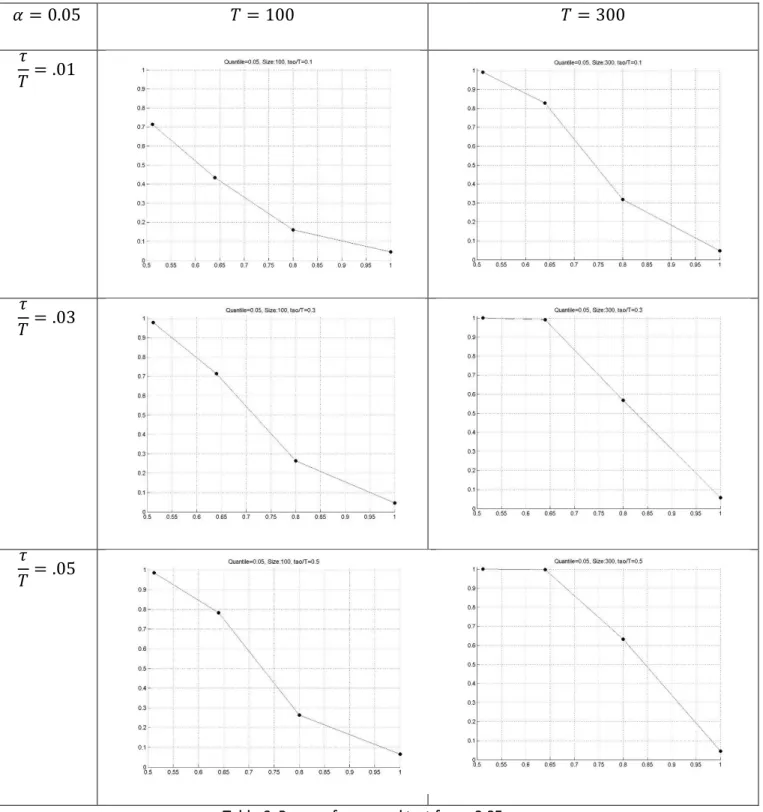
4.4 Power of the test
Power of the test allows us to analyze the performance of the test, this is, verify is the test
rejects the null hypothesis when alternative hypothesis is correct. To accomplish this
proposed test must be executed under stages when variances change (alternative
hypothesis). Thus the power of the test was calculated with all the combination of the next
stages.
Size of the series (T) of 20,30,100,300
Change point localization ( ) of 0.1, 0.3 and 0.5
Shifts in variance ⁄ of and
Each stage is replicated 1000 times and the probability is calculated by the times that
null hypothesis is rejected divided by 1000.
To achieve this we used a Matlab® script. The results were saved as excel tables and jpg
pictures. The time of execution for this program was 7783.116291 seconds.
Table 6 and 7 show the results for specific stages for two tails. Horizontal axis represents
shifts in variance and vertical axis represents the probability of rejecting the null
hypothesis.
29
30
Table 7: Power of Proposed test for α=0.95
Note that when variance is equal to 1 the probability of rejecting the null hypothesis is
almost equal to the significance level. This indicates that simulated quantiles are closely
31 the shift in variance is located in the half of the series. In the same way power increases
when size increases.
4.5 Comparison with Chen’s Test 1997 .
In 1997 Jie Chen and K. Gupta wrote an article proposing a Hypothesis Test for shift in
variance. They used the Schwarz Information Criterion (SIC) defined as ( ̂)
where ( ̂) is the maximum likelihood function for the model, is the number of free parameters in the model and is the sample size.
They accept if and reject when
where:
The number is the change point and is obtained from table 8.
Size
20 19.106 9.691 6.698
50 17.284 9.171 6.208
100 16.280 8.626 5.799
200 15.416 8.088 5.359
Table 8: Values of
The power of this test was calculated for these stages, power of proposed test was
calculated for T=200 and results were compared. Table 9 shows the results of the
comparison for size 200 and significance level of .05. Note that the power of proposed test
32 Parameters
(Quantile, size, )
Chen Proposed
(0.05, 200, .1)
(0.05, 200, .3)
(0.05, 200, .5)
33 (0.95, 200, .3)
(0.95, 200, .5)
Table 9: Comparison between Chen's test and Proposed's test.
Observe that the test developed in this research accepts the null hypothesis more times
when it is true because the height lowest point (where there is no change in variance) is
more near to the significance level. In the other hand, this test rejects more times the null
hypothesis when it is false, indicated by the bigger height of the other 3 points.
Based on these observations we can ensure than proposed test has a better performance
tha Che ’s test.
4.6. – Numerical Example
The S&P 500 (the “ta da d a d Poo ’s 5 ), is one of the most used American stock index.
Figure 5 shows data between July 2004 and July 2009. In this figure, the reader can
graphically observe a decrease in the variance. The proposed test was applied with
significance level of .05. Null hypothesis was rejected and the change-point (red) was
estimated in the 23rd observation. This result is very similar to the obtained by Villanueva
35
CONCLUSIONS AND FUTURE WORK
Conclusions
There are not ideal processes, this is, every process presents variability. In the other hand
quality is defined as the reduction of variability. Therefore is necessary to monitor the
variability of a process in order to design strategies to reduce it. In spite of this Change
Point Analysis researchers have dedicated most of the efforts to detect change points in
mean. Due to this, a hypothesis test based on p values of F distribution was designed to
detect shifts in variances
The first conclusion is that this hypothesis test has proved its efficiency for detecting
changes in variances for simulated data as we can see in sections 4.4. Moreover the test
epo ted ette esults tha Che ’s test, hi h effi ie is e si ila to CUM“UM as we
can see in section 4.5. With these two results the research hypotheses stated in section 1.5
are proved.
A remarkable fact is that the regression curves are the best ones found in the literature,
reporting maximum absolute errors near of a ten millionth for sample sizes bigger than 50.
This method offers the following advantages if it is compared with the most common
existent techniques.
Computing time of Control Charts is very high. The execution time of the numerical
example was of 0.002799 seconds making this tool able to use in production lines.
GLR based tools like Chen test (1997) are not very accurate. As was shown in
section 4.5 this method offered better results.
Statistic test like proposed by Hawkins (2005) assume data with the same
distribution. This test uses F distribution for different parameters in each step.
The main disadvantage of this tool is that it works only with normal series of independent
36 Future work
To continue enriching the present work the following two lines are suggested.
First, as was mentioned in subsection 4.2, the exact distribution of the proposed statistic is
unknown yet. Theoretical asymptotical properties of this statistic can be obtained.
Second, this methodology can be extended to use P-values for other distributions to design
hypothesis tests for detecting shifts not only in variance but also in mean. This is, taking the
general model.
{
With the Hypotheses and
Applying the Likelihood Ratio Test for all we can obtain and
and their respective quantiles in the same way proposed in this work.
A particular case is to use the p-values of the chi squared distribution in the next way.
Let be a set of independent observations following the next distribution:
{
Parameters and are known and is unknown. Hypotheses are
and .
The likelihood ratio for this test is based on the statistic
The P –value is obtained from the next equation
( )
37
̂
To summarize, there is opportunity to continue researching the application of P-values to
38
REFERENCES
Amiri, A., & Allahyari, S. (2011). Change Point Estimation Methods for Control Chart
Postsignal Diagnostics: A Literature Review. Quality and Reliability Engineering
International, 1-13.
Bhattacharya, P. (1994). Some Aspects of Change-Point Analysis. Lecture Notes-Monograph
Series, Vol. 23, Change-Point Problems, 28-56.
Casella, G., & Berger, R. (2002). Statistical Inference. Pacific Grove, CA USA: Thomson
Learning.
Chen, J., & Gupta. (2001). ON CHANGE POINT DETECTION AND ESTIMATION.
Communications in Statistics - Simulation and Computation, 665-697.
Chen, J., & Gupta, A. (1997). Testing and Locating Variance Changepoints With Application
to Stock Prices. Journal of the American Statistical Association, 739-747.
Cordero, A. T., & Gonzalez, R. (2012). Generalized Control Chart for Variance Based on the
P-Value of Chi square Test. Proceedings of the 2012 Industrial and Systems
Engineering Research Conference, 1-5.
Devore, J. (2008). Probabilidad y estadistica para ingenieria y ciencias. Mexico City, Mexico:
Cengage Learning Editores.
Fotopoulos, S., Jandhyala, V., & Kahpalova, E. (2010). EXACT ASYMPTOTIC DISTRIBUTION OF
CHANGE-POINT MLE FOR CHANGE IN THE MEAN OF GAUSSIAN SEQUENCES. The
Annals of Applied Statistics, 1081–1104.
Freund, J., & Miller, I. M. (1999). Estadistica Matematica con Aplicaciones. New Jersey,
39 Garza, J. (2013). ANALYSIS OF MULTIPLE CHANGE-POINTS IN NORMALLY DISTRIBUTED
SERIES. San Nicolas Mexico: UANL.
Hawkins, D. (1977). Testing a Sequence of Observations for a Shift in Location. Journal of
the American Statistical Association, 180-186.
Hawkins, D., & Zamba, K. (2005). A Change-Point Model for a Shift in Variance. Journal of
Quality Technology, 21-31.
Hawkins, D., Qiu, P., & Wook, C. (2003). The Changepoint Model for Statistical Process
Control. Journal of Quality Technology, 355-366.
Hinkley, D. (1970). Inference About the Change-Point in a Sequence of Random Variables.
Biometrika, 1-17.
Inclan, K., & Tiao, G. (1994). Use of Cumulative Sums of Squares for Retrospective
Detection of Changes of Variance. Journal of the American Statistical Association,
913-923.
Page, E. (1954). Continuous Inspection Schemes. Biometrika, 100-115.
Page, E. (1955). A Test for a Change in a Parameter Occurring at an Unknown Point.
Biometrika, 523-527.
Page, E. (1957). On Problems in which a Change in a Parameter Occurs at an Unknown
Point. Biometrika, 248-252.
Perez, A. (2013). Dete ió del Pu to de Ca io Media te el Uso “e uencial de Cartas de
Control y Estimadores de Máxima Verosimilitud. San Nicolas Nuevo Leon Mexico:
40 Pettitt, A. (1979). A Non-Parametric Approach to the Change-Point Problem. Journal of the
Royal Statistical Society, 126-135.
Samuel, T., Pigniatello, J., & Calvin, J. (1998). IDENTIFYING THE TIME OF A STEP CHANGE
WITH CONTROL CHARTS. Quality Engineering, 521-527.
Sen, A., & Srivastava, M. (1975). On tests for detecting change in mean. The Annals of
Statistics, 98-108.
Tercero, V. G., Garza, J., & Cordero, E. (2013). Likelihood Ratio Test for a Change-Point in
the Mean of Independent Normal Observations. Proceedings of the 2013 Industrial
and Systems Engineering Research Conference, 1-8.
Tercero, V., Martinez, I., & Ramirez, J. (2012). Change-Point Estimation and Control Chart
for Variance Based on the P-Value Function of the F statistic. Proceedings of the
2012 Industrial and Systems Engineering Research Conference, 1-8.
Villanueva, C. (2013). Carta de Control No-Paramétrica de Punto de Cambio para Varianza.
San Nicolas Mexico: UANL.
Zhou, C., Zou, C., Zhang, Y., & Wang, Z. (2009). Nonparametric control chart based on
41
APPENDIX
A.1 Matlab codes
A.1.1 Quantile estimation
clc
42 filename = 'distf500.xlsx';
xlswrite(filename,result)
A.1.2 Power of the test
tic clc clearvars image=0; alpha(:,1)=[.01,.05,.1,.2]; alpha(:,2)=[.8,.9,.95,.99]; varshift(:,1)=[1,1/1.25,1/1.25^2,1/1.25^3]; varshift(:,2)=[1,1.25,1.25^2,1.25^3];
twenty(:,1)=[0.000859101 0.005585629 0.011574396 0.0322866]; twenty(:,2)=[0.967915639 0.98763408 0.994482116 0.999329755]; fifty(:,1)=[0.000350961 0.004021736 0.009062285 0.021870338]; fifty(:,2)=[0.980962703 0.993302279 0.996933472 0.999431223]; a1(:,1)=[.0215 .1259 .2773 .6848];
a1(:,2)=[-.7059 -.2788 -.1172 -.0184]; a2(:,1)=[.002 .0013 .0032 .0079]; a2(:,2)=[.9918 .9967 .9986 .9998]; T=[20,50,100,300]; changePos=[.1,.3,.5]; cont=zeros(1,4); for cola=1:2 for a=1:4 for size=1:4 for tonT=1:3 change=changePos(tonT)*T(size); for rep=1:1000 if size==1 s=twenty(a,cola); elseif size==2 s=fifty(a,cola); else
s=a1(a,cola)/T(size) + a2(a,cola); end
x=zeros(1,T(size)); for var =1:4
for i=1:change x(i)=randn; end for i=change+1:T(size) x(i)=varshift(var,cola)*randn; end miu0=zeros(T(size),1); miu1=zeros(T(size),1); sigma0=zeros(T(size),1); sigma1=zeros(T(size),1); r=zeros(T(size)-4,1); v1=zeros(T(size)-4,1); v2=zeros(T(size)-4,1); p=zeros(T(size)-4,1); for k = 3:T(size)-2 for i=1:k
43 end miu0(k)=miu0(k)/k; for i=1:k sigma0(k)=sigma0(k)+(x(i)-miu0(k))^2; end sigma0(k)=sigma0(k)/(k-1); for i=(k+1):T(size) miu1(k)=miu1(k)+x(i); end miu1(k)=miu1(k)/(T(size)-k); for i=(k+1):T(size) sigma1(k)=sigma1(k)+(x(i)-miu1(k))^2; end sigma1(k)=sigma1(k)/(T(size)-1-k); r(k-2)=sigma1(k)/sigma0(k); v1(k-2)=T(size)-1-k; v2(k-2)=k-1; p(k-2)=fcdf(r(k-2),v1(k-2),v2(k-2)); end if cola==2 pv=max(p); if pv>s cont(var)=cont(var)+1; end else pv=min(p); if pv<s cont(var)=cont(var)+1; end end end end cont=cont/rep; image=image+1; name=strcat('Quantile= ',num2str(alpha(a,cola)),... ', Size: ',num2str(T(size)),', tao/T= ',num2str(changePos(tonT))); xlswrite(num2str(image),cont); figure scatter(varshift(:,cola),cont,'k','filled') title(name); hold on plot(varshift(:,cola),cont,'b') hold on ylim([0 1.01]) grid on saveas(gcf,num2str(image),'jpg') end end end end toc
A.1.3 Comparison for decreasing variance
tic clc
44 image=0;
alpha(:,1)=[.01,.05,.1];
varshift(:,1)=[1,1/1.25,1/1.25^2,1/1.25^3]; twenty(:,1)=[19.106 9.961 6.698];
fifty(:,1)=[17.284 9.171 6.208]; hundred(:,1)=[16.280 8.626 5.799]; twohundred(:,1)=[15.416 8.088 5.359]; T=[20,50,100,200]; changePos=[.1,.3,.5]; cont=zeros(1,4); cola=1; for a=1:3%3 for size=1:4%4 for tonT=1:3%3 change=changePos(tonT)*T(size); for rep=1:1000 if size==1 ca=twenty(a,cola); elseif size==2 ca=fifty(a,cola); elseif size==3 ca=hundred(a,cola); elseif size==4 ca=twohundred(a,cola); end x=zeros(1,T(size)); for var =1:4
45 sigma1(k)=sigma1(k)/(T(size)-1-k); sick(k-2)=T(size)*log(2*pi)+k*log(sigma0(k))+... (T(size)-k)*log(sigma1(k))+T(size)+2*log(T(size)); end miu=0; sigma=0; for i=1:T(size) miu=miu+x(i); end miu=miu/T(size); for i=1:T(size) sigma=sigma+(x(i)-miu)^2; end sigma=sigma/(T(size)-1); sicn=T(size)*log(2*pi)+T(size)*log(sigma)+T(size)+log(T(size)); sic=min(sick); if sicn>(sic+ca) cont(var)=cont(var)+1; end end end cont=cont/rep; image=image+1; name=strcat('Quantile= ',num2str(alpha(a,cola)),',... Size: ',num2str(T(size)),', tao/T= ',num2str(changePos(tonT))); % xlswrite(num2str(image),cont);
figure scatter(varshift(:,cola),cont,'k','filled') title(name); hold on plot(varshift(:,cola),cont,'b') hold on ylim([0 1.01]) grid on saveas(gcf,num2str(image),'jpg') end end end toc
A.1.4 Comparison for increasing variance
tic clc clearvars image=0; alpha(:,1)=[.01,.05,.1]; varshift(:,1)=[1,1.25,1.25^2,1.25^3]; twenty(:,1)=[19.106 9.961 6.698]; fifty(:,1)=[17.284 9.171 6.208]; hundred(:,1)=[16.280 8.626 5.799]; twohundred(:,1)=[15.416 8.088 5.359]; T=[20,50,100,200];
46 for a=1:3%3
for size=1:4%4 for tonT=1:3%3
change=changePos(tonT)*T(size); for rep=1:1000
if size==1
ca=twenty(a,cola); elseif size==2
ca=fifty(a,cola); elseif size==3
ca=hundred(a,cola); elseif size==4
ca=twohundred(a,cola); end
x=zeros(1,T(size)); for var =1:4
for i=1:change x(i)=randn; end
for i=change+1:T(size)
x(i)=varshift(var,cola)*randn; end x=fliplr(x); miu0=zeros(T(size),1); miu1=zeros(T(size),1); sigma0=zeros(T(size),1); sigma1=zeros(T(size),1); r=zeros(T(size)-4,1); v1=zeros(T(size)-4,1); v2=zeros(T(size)-4,1); sick=zeros(T(size)-4,1); for k = 3:T(size)-2 for i=1:k
miu0(k)=miu0(k)+x(i); end
miu0(k)=miu0(k)/k; for i=1:k
sigma0(k)=sigma0(k)+(x(i)-miu0(k))^2; end
sigma0(k)=sigma0(k)/(k-1); for i=(k+1):T(size)
miu1(k)=miu1(k)+x(i); end
miu1(k)=miu1(k)/(T(size)-k); for i=(k+1):T(size)
sigma1(k)=sigma1(k)+(x(i)-miu1(k))^2; end sigma1(k)=sigma1(k)/(T(size)-1-k); sick(k-2)=T(size)*log(2*pi)+k*log(sigma0(k))... +(T(size)-k)*log(sigma1(k))+T(size)+2*log(T(size)); end miu=0; sigma=0;
for i=1:T(size) miu=miu+x(i); end
47 for i=1:T(size)
sigma=sigma+(x(i)-miu)^2; end sigma=sigma/(T(size)-1); sicn=T(size)*log(2*pi)+T(size)*log(sigma)+T(size)+log(T(size)); sic=min(sick);
if sicn>(sic+ca)
cont(var)=cont(var)+1; end end end cont=cont/rep; image=image+1;
name=strcat('Quantile= ',num2str(1-alpha(a,cola)),...
', Size: ',num2str(T(size)),', tao/T= ',num2str(changePos(tonT)));
% xlswrite(num2str(image),cont);
figure
scatter(varshift(:,cola),cont,'k','filled') title(name);
hold on
plot(varshift(:,cola),cont,'b') hold on
ylim([0 1.01]) grid on
saveas(gcf,num2str(image),'jpg') end
end
end
toc
A 1.5 Numerical Example
clearvars clc
tic
x=[-6.36 31.4 13.19 77.65 92.64 -18.84 -79.67 -8.63 17.88 23.47 -40.65 70.46 9.79 77.32 78.2 -4.45 100.79 -70.48 -50.55 56.49 24.12 14.55 -7.03 -68.74 -46.67 -10.91 -15.81 -17.7 12.05 -54.75 -7.49 -53.71 -19.21 -13.81 18.73 18.91 13.38 20.15 39.12 2.52 10.35 15.62 43.63 38.09 30.65 -22.33 23.01 23.74 -34.65 0.17 -42.85 13.85 -8.48 21.81 -42.47 1.19 -31.79 -0.58 -14.16 -15.78 40.52];