Contaduría y Administración 63 (1), 2018, 1-28 Accounting & Management
Social accounting matrix and analysis of productive
sectors in Mexico
Matriz de contabilidad social y análisis de sectores
productivos en México
Gaspar Núñez Rodríguez
El Colegio de México, MéxicoReceived 14 october 2015; accepted 14 october 2016 Available online 11 december 2017
Abstract
Although the Social Accounting Matrix (SAM) began to be developed almost half a century ago, and many countries have developed a SAM for their own economy, a considerable delay has been observed in Mexico. While different researchers have built a SAM, oftentimes it is not possible to validate or replicate their results, as the matrix is not published. The main objective of this work is to propose a specific metho -dology for the case of Mexico, and to build a SAM for the year 2003 in a transparent manner. Therefore, the proposed methodology can be discussed (improved or rectified) to apply it to the construction of broad or updated matrices for the Mexican economy, in accordance with the Mexican System of National Accounts. For its part, the SAM can be used to carry out different analyses for this period, whether structural, of Applied General Equilibrium (AGE), or others; the results of which can be replicated and thus be corroborated or rectified. Therefore, as a second objective, we used the SAM to carry out a basic characterization of the productive structure, and we calculated the General Multipliers Matrix, calculating the carry-over and dispersion indices to determine the relative importance of the sectors, and identify key and strategic sectors.
JEL Classification: C67, D57, D58
Keywords: Input - Output Table ; Social Accounting Matrix; Mexico; General Multipliers; Rasmussen Indices.
https://doi.org/10.22201/fca.24488410e.2018.873
0186- 1042/© 2018 Universidad Nacional Autónoma de México, Facultad de Contaduría y Administración. This is an open access article under the CC BY-NC-ND (http://creativecommons.org/licenses/by-nc-nd/4.0/).
E-mail address: [email protected]
Resumen
Aunque hace casi medio siglo que la Matriz de Contabilidad Social (MCS) comenzó a desarrollarse, y muchos países han elaborado una MCS para su economía, en México se ha observado un considerable atraso. Aunque diversos investigadores han construido su MCS, con frecuencia no es posible validarla ni replicar sus resultados, pues la matriz no se publica. El principal objetivo del presente trabajo es el de plantear una metodología específica para el caso de México, y construir de forma transparente, una MCS para el año 2003. La metodología propuesta, por tanto, puede ser discutida (mejorada o rectificada) para aplicarla a la construcción de matrices ampliadas o actualizadas de la economía mexicana, en concor-dancia con el Sistema de Cuentas Nacionales de México. La MCS por su parte, puede ser utilizada para llevar a cabo diversos análisis para este periodo, ya sean estructurales, de equilibrio general aplicado, u otros, cuyos resultados puedan replicarse y por tanto corroborarse o rectificarse; por ello, como segundo objetivo, utilizamos la MCS, para realizar una caracterización básica de la estructura productiva, y com-putamos la Matriz de Multiplicadores Generalizados, calculando los índices de arrastre y dispersión para determinar la importancia relativa de los sectores, e identificar sectores clave y estratégicos.
Códigos JEL: C67, D57, D58
Palabras clave: Matriz Insumo-Producto. Matriz de Contabilidad Social. México, Multiplicadores Generalizados.
Introduction1
The structural analysis, derived for the most part from the Leontief model, has been
developed throughout more than eight decades since the first works by Leontief (1936), and it
is one of the methodologies used for the empirical analysis of real economies and for the design
of economic policies. Virtually all the structural analysis tools—at first developed for the
input-product analysis—can also be applied to the social accounting matrices.
However, despite the fact that the concept of Social Accounting Matrix (SAM) was developed and began to gain importance almost half a century ago, with at least one SAM having been developed in most countries based on the National Accounts, Mexico has had a marked backwardness due to various reasons—perhaps the main of which being that the INEGI abandoned the development of the Input - Output Table (IOT) for more than 30 years—, so that currently and in most cases each researcher in this area develops their own SAM, without the possibility of replicating the results, given that the SAM is not generally published. The main objective of this work is to build and present a SAM of the Mexican economy for the year
2003, based on the Domestic Input-Output Symmetric Table for the Total Economy, officially
published by the INEGI, and using a transparent methodology, so that it can be used to carry out research with results that can be replicated and corroborated (or corrected). Furthermore, we did a basic study for the characterization of the productive sectors, and concluded with an application using the Leontief model to obtain the General Multipliers Matrix (GMM), with which we analyzed the structure of the productive sector of the country, and calculated the carry-over and dispersion indices to determine the relative importance of the productive activities in the Mexican economy.
While it is true that the OIT for 2008 is already available as well as an update for 2012,2 and therefore it is possible to update the SAM, this in no way undermines the usefulness and interest for a SAM for 2003 for various reasons.
Without being exhaustive, one of these is that the study of the evolution of variables throughout time is one of the fundamental interests of the economic analysis (this is the reason for the construction of time series), and the comparative studies of a set of data in two points of time is one of the basic approaches to the topic.
Another is that, insofar as the structural changes on the economy are not significant
throughout a determined period, the conclusions could maintain their validity and, if there are
indeed significant changes, their study could help understand how the different transmission
mechanisms act on the economy.
In the practical field, the evaluation of the results of public policies and programs requires
analyzing scenarios a posteriori (or ex post), regarding initial or reference situations, for which a SAM prior to the scenario of interest is of obvious importance.
Moreover, the fact that a set of data corresponds to a past period does not necessarily invalidate the results that could be derived from these. In other words, most (or all) of the work and the results obtained by past scientists, would lack validity.
On the other hand, the construction of this SAM is also intended to contribute elements that allow—along with the eventual contributions of other researchers interested in the topic—
defining the methodology, or the most appropriate approach for the construction of Mexico’s
SAM; both because the inter-temporal comparability is of central importance for the analysis of the evolution of variables, and because if each researcher builds their own database, then the
results would not be comparable and thus, would be difficult to verify.
This work closely follows the methodology developed by Núñez (2014) for the construction of a macro-SAM, that is, an aggregated matrix at the macroeconomic level for the Mexican economy, and based on this macro-SAM we built the micro-SAM reported here. Furthermore, in this work we carried out a basic characterization of the productive structure, and calculated the General Multipliers Matrix, calculating the carry-over and dispersion indices to determine the relative importance of the sectors, and to identify key and strategic sectors.
We consider that the main advantage of this work is that it proposes a specific methodology
for the Mexican System of National Accounts (MSNA), departing from the Input - Output Table (OIT) published by the INEGI, and data from the national accounts, to build a transparent SAM
that can be replicated and corrected, or modified to carry out different researches; because as far
as we know, this has not been done for Mexico, given that according to the work of Barbosa-Carrasco et al. (2009):
“Despite its importance, there is no official SAM for Mexico and each researcher builds their own: 1) A SAM, in 1975, to analyze the function of the public sector in the economy of the country (Pleskovic and Treviño, 1985); 2) a SAM, with data from 1989, to calibrate the model to evaluate the impact of Mexico trade openness (Levy and Van Wijnbergen, 1992); 3) a SAM, based on 1985, to calibrate the computable general balance models to analyze the consequences of the North Ame-rican Free Trade Agreement and fiscal policies (Sobarzo, 1992 and 1994); and 4) a SAM with data from 1996 (Harris and Robinson, 2003) (McDonald and Thierfelder, 2004). Of these matrices, only those by Pleskovic and Treviño (1975), Harris and Robinson (2003), and a SAM of the
GTAP with data from 1997 (Trejos et al., 2004) were published. Due to there not being a more recent SAM that is available for Mexico, this work was done with the objective of building one for 2004”.
More recent works such as that by Aguayo et al. (2009) are based on updates made to considerably old matrices,3 and others such as the cited work of Barbosa-Carrazco et al. (2009) resort to econometric techniques to estimate a great quantity of unavailable data.4 The proposal followed in this work allows building a SAM based on current and complete data, therefore, it is possible to apply this methodology to the 2008 input-product matrices, and to the 2012 update published by the INEGI,5 as well as to future matrices and supplementary data of the national accounts, without having to resort to updating old data or estimating inexistent data.
Both works cited in this paragraph—published in the same year (2009), regarding two matrices
for the same year (2004), built with different methodologies, and thus non-comparable—also show the need for a consistent approach that avoids the duplication of efforts and, above all, the need to have a framework that allows replicating and comparing the results of different researches.
The article is organized as follows. In the first section, we considered the matrix to be
used and we take the Domestic Input-Output Symmetric Table(OIT-Mx03ETD), adding the productive sectors to obtain the macro matrix from which the SAM-Mx03 will be built. In the second section, the Activities are disaggregated to carry out the basic study of the sectors and their characterization. In the third section, we select the exogenous accounts and apply the Leontief model to obtain the General Multipliers Matrix (GMM) and elaborat the Rasmussen indices. Finally, the fourth section presents some closing remarks.
Construction of the Social Accounting Matrix SAM-Mx03.
Table 1 partially compares, from the production point of view, the 4 input-product symmetric matrices published by the INEGI. The basic differences consist, on the one hand, on the disaggregation done on the imports, and on the other, the Maquila Export Industry (MEI). For this work, we have opted to use the Domestic Input-Output Symmetric Table for the Total Economy (OIT-Mx03ETD, which simply follows the OIT), given that the additional objective will be to carry out a sector analysis. The methodology used is immediately applicable to any of the other input-product matrices of Table 1 for the construction of the corresponding SAM.
Throughout the article, the figures are expressed in millions of pesos for the year 2003, unlike
the national accounts, where these are expressed in thousands of pesos.
3 “The technical coefficient matrix is an update of the one corresponding to the OIT Mexico 1993...” (Aguayo
et al., 2009).
4 In this case, Barbosa-Carrasco et al. (2009) use a cross-entropy method.
Table 1
Input-Output Symmetric Tables 2003 of the INEGI. (Millions of pesos). Total Economy Total Symmetric Matrix
Internal Economy Total Symmetric Matrix
Total Economy Domestic Symmetric Matrix
Internal Economy Domestic Symmetric Matrix
Uses of the Internal Economy of national origin 3 720 327
Uses of the MEI of national origin 86 669
Uses of the Internal Economy of national origin
and import 4 495 139
Total uses of national origin 3 806 997 3 806 997
Imports of the Internal Economy 774 811
Imports of the MEI 637 968
Uses of the MEI of national origin and import 724 638
Imports of the Total Economy 1 412 780 1 412 780
Total uses of national origin and import 5 219 776 5 219 776 5 219 776 5 219 776
Taxes on net products and subsidies 36 773 36 773 36 773 36 773
Total uses of national origin and import at
purchaser price 5 256 549 5 256 549 5 256 549 5 256 549
Gross Value Added Internal Economy 7 055 776 7 055 776
Gross Value Added MEI 112 749 112 749
Gross Value Added Total Economy 7 168 526 7 168 526 7 168 526 7 168 526
Production of the Internal Economy At basic prices 11 587 688 11 587 688
Production of the MEI At basic prices 837 387 837 387
Production of the Total Economy At basic prices
12 425 075 12 425 075 12 425 075 12 425 075
GDP of the Internal Economy 7 092 549 7 092 549
GDP of the MEI 112 749 112 749
GDP of the Total Economy 7 205 299 7 205 299
Source: Own elaboration based on the Mexican Input-Product Matrices for 2003 (INEGI, 2008). Elaboration of the macro matrix.
First, we added the 20 sectors of the OIT into a single one to facilitate the elaboration of the macro matrix, since once this is squared, according to the national accounts, the subsequent disaggregation will maintain the consistency. The OIT with the aggregated productive sectors is shown in Table 2.
Although the SAM can be seen as an extension of the OIT, conceptually, it is an accounting framework that has two fundamentally different implications: while the OIT focuses on the productive sectors, specifying all of their inputs and the destination of the production, the SAM
economy, focusing on the institutions of the same (namely, Households, Government, and Companies or Partnerships, thus it is denominated Social Accounting Matrix) and thus on the balance of the economy as a whole. Consequently, the SAM contains more information than the OIT due to necessity. Furthermore, according to the conventional standard format, each
account has a row that specifies its incomes (resources) and a column that specifies its expenses
(uses); meaning that the SAM is a squared matrix where the total per row is exactly the same
as the total per column (income=expense) (Defourney and Thorbecke, 1984). Table 3 shows
the information of the OIT contained in Table 2, using the previously mentioned standard SAM format.
Table 2
OIT with the added productive sectors into a single one. (Millions of pesos). Activities Private
Consumption Government Consumption FBCF Variation of Stocks FOB Export Total Final Consumption Internal Production Basic Prices Activities 3 806 997 4 476 438 892 322 1 200 864 235 250 1 813 205 8 618 079 12 425 075
Imports 1 412 780 255 514 402 225 414 63 482 544 812 1 957 592
Net purchases, residents and non-residents.
-35 084 1 120 102 560 68 597 68 597
Total Imports 1 412 780 220 430 1 523 225 414 63 482 102 560 613 409 2 026 188 Taxes on Net
products of subsidies
36 773 351 640 4 617 356 257 393 030
Total uses
purchaser prices 5 256 549 5 048 508 893 844 1 430 894 298 732 1 915 766 9 587 744 14 844 294 Gross Value
Added of the Total Economy
7 168 526
Production Total Economy
Basic prices
12 425 075
Gross Domestic Product of the Total Economy
7 205 299 351 640 4 617 356 257 7 561 556
Table 3
Data from the OIT-Mx03ETD in standard SAM format. (Millions of pesos.) Private
consumption (Households)
Government consumption (Government)
FBCF and Change in Stocks (Investment)
Productive Sectors (Activities)
Exports
(RoW) Row Total (Resources)
Private consumption (Households)
7 168 526 7 168 526
Public consumption (Government)
351 640 4 617 36 773 393 030
FBCF and Change in Stocks (Savings)
0
Productive Sectors (Activities)
4 476 438 892 322 1 436 114 3 806 997 1 813 205 12 425 075
Imports (RoW) 220 430 1 523 288 896 1 412 780 102 560 2 026 188
Column Total
(Uses) 5 048 508 893 844 1 729 627 12 425 075 1 915 766
Source: Own elaboration based on Table 1.2.
Table 3 makes obvious that with the information from the OIT, only the account of the productive Activities is balanced. All the others show greater or lesser imbalances, because the OIT does not contain the necessary information that must be integrated into the SAM. For example, in the case of Households, the incomes must also include the transfers and payments of the RoW to the productive factors, and for expenses, the taxes paid by the households must also be included, mainly the ISR. In the case of the Government, there are also certain elements missing with regard to its income and others regarding public expenses, and such is the case for the other accounts. In other words, the difference between a SAM and a OIT is both conceptual and informative, and not a matter of format, thus, it is not possible to make an OIT using the SAM format.
Subsequently, we resort to the data of the Mexican System of National Accounts (MSNA) to balance the accounts of the matrix in Table 3, to obtain a squared (balanced) macro matrix, from which we can build a fully consistent micro matrix. During the process, we will introduce new accounts to build a matrix that adequately shows the data of our economy, resorting mainly to the data reported in the Goods and Services Accounts (Inegi, 2010a) and the Accounts by Institutional Sector (Inegi, 2010b). The macro matrix obtained is shown in Table 4.
Following the order proposed in Table 3, we begin with the balance of the account for the Households. For this, it is necessary to previously introduce three more accounts: the Capital and Labor to disaggregate the Value Added, and the Partnerships to systematically make use of the data of the Accounts by Institutional Sectors (AIS).
According to Table 3 of the Goods and Services Accounts (GSA) Employee remuneration (including Social contributions) increases to 2 370 474 (as noted above, all figures are in millions of pesos for 2003), and the Gross operating surplus (GOS) increases to 4 487 421.
of the total economy reported by the OIT gives us 310 631, which are the Other taxes on production paid by the Activities to the Government (in addition to the net taxes on the products already mentioned). The GOS goes to the Capital account, which transfers it to the Partnerships, which shall subsequently distribute it. The Employee remuneration goes to the Labor account, minus the Social contributions that the Activities pay to the Government, given that according to the AIS the “Net social contributions” perceived by the government are of 147 621, and thus the remaining 2 222 853 must correspond to the Households.
On the other hand, according to the AIS, the Social transfers (Social benefits different to the transfers in kind) are of 117 510, from which we subtract the Other social transfers (net) 4 269, to obtain the total transfers that the government makes to the Households: 113 241. In this case, we wish to obtain only the gross income of the Households, thus we subtract the Other social transfers that the government makes.
Also, according to the AIS the Other current transfers (net) of the RoW are of 167 223, (which constitute the remittances that the Households receive), and the payment of the RoW to the labor factor is of 16 353, with which the Households incomes are completed, missing only what they receive as capital income (GOS) from the partnerships.
Before obtaining the GOS that the Households receive from the Partnerships, we can observe their additional expenses to obtain their GOS as a balance. According to the AIS the Gross savings of the Partnerships is of 779 607, of 116 046 for Government, of 757 902 for the Households and the ISFLSH, and of 76 071 for the RoW.
Finally, according to the AIS, the ISR paid by the Households is of 226 509, (in addition to the consumer tax mentioned above). The ISR paid by the Partnerships (financial and non-financial) is of 170 107.
Since we already have the total expenses of the Households, and all of the elements of their
income, we can obtain the GOS they obtain as the difference given by the balance: 3 513 249,
with which the Households account is balanced.
The next account is that of Partnerships, for which we have practically obtained all the elements, observing that it has a balance of 24 458 corresponding to the Property income that the Partnerships pay to the RoW, which is consistent with the AIS data. With this, the Partnerships account is now also balanced.
Here we can observe that all the other accounts are already balanced, except that of Government, showing an imbalance of 124 766, which corresponds to the payment of the Property income of the Government to the RoW. It is worth noting that this payment, plus the
payment made by the Partnerships that we obtained previously, add up to 149 224, an amount
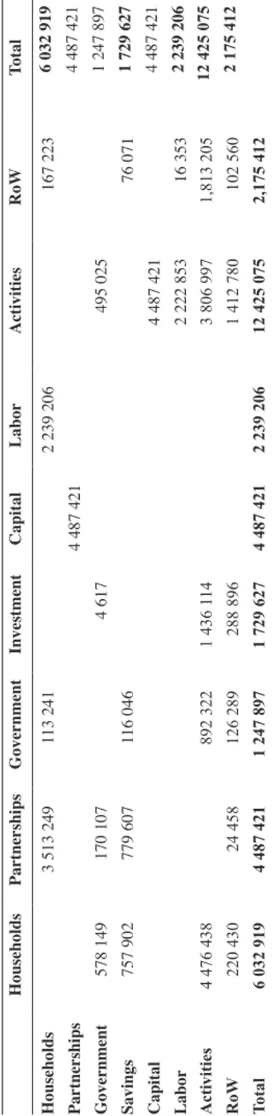
Table 4 Social
Accounting Macro Matrix. (Millions of pesos).
Households
Partnerships
Government
Investment
Capital
Labor
Activities
RoW
Total
Households
3 513 249
113 241
2 239 206
167 223
6 032 919
Partnerships
4 487 421
4 487 421
Government
578 149
170 107
4 617
495 025
1 247 897
Savings
757 902
779 607
116 046
76 071
1 729 627
Capital
4 487 421
4 487 421
Labor
2 222 853
16 353
2 239 206
Activities
4 476 438
892 322
1 436 1
14
3 806 997
1,813 205
12 425 075
RoW
220 430
24 458
126 289
288 896
1 412 780
102 560
2 175 412
Total
6 032 919
4 487 421
1 247 897
1 729 627
4 487 421
2 239 206
12 425 075
2,175 412
Source: Own elaboration with data from the Mexican System of National
Disaggregation of the Activities and basic characterization.
To disaggregate the Activities, we return to the OIT to reestablish the data that we added to elaborate the macro matrix, and shall subsequently use the information of the GSA to disaggregate the remaining data.
Previously, we introduced four more accounts to separate the social taxes (ISR, Social contributions, Sale taxes, and Other taxes on the production) to adequately carry out their disaggregation by productive sector.
Once the taxes have been reorganized, we open the 20 accounts necessary to disaggregate the Activities, where we can immediately copy the data from the OIT: inter-industrial exchanges submatrix, and the columns for Private Consumption, Government Consumption, FBCF plus Change in Stocks, and Exports. This done, the assignment of all the goods and services provided by the Total supply is completely disaggregated.
We can also immediately disaggregate the data from the rows of Imports and Sales Tax, copying the data from the OIT to the SAM, thus including in the SAM all the information of the IMP that is advantageous for its construction as has been mentioned, and we proceed to using the data reported by the GSAs.
Tables 55, 58, and 59 of the GSAs contain figures, by productive sector, of the Employee
remuneration, of the Other taxes on the production, and the GOS respectively. As in said tables
sectors 48 and 49 are aggregated, and considering that the importance of sector 49 is relatively
small to maintain the transparency of the data, we also added these two sectors to the SAM (it is always possible to disaggregate them later if the necessary information becomes available).
The three listings mentioned comprise the Gross Value Added (GVA), however, unlike the
IMP, the GOS reported in the GSAs includes the “Indirectly measured financial intermediation services”, which are not disaggregated. Therefore, to calculate the GOS per Activity, we first
added the Remunerations, the Other taxes, and the GOS of the GSAs to obtain a GVA that includes the Financial services, and subsequently subtracted the GVA from the IMP to obtain the Financial services per sector, which we in turn subtracted from the GOS of the GSAs to obtain the net GOS per Activity of the Financial services.
The Other taxes on production in Table 58 of the GSA are the net taxes (304,878), which differ from those calculated for the macro matrix (310 631); this is a relatively small (1.85%) unexplained difference, and to distribute it we assume that it is proportionally allocated between the sectors.
On the other hand, we must separate the Social contributions from the Remunerations, for which we will also assume that the payment of the Social contributions is proportional to the Remunerations paid by each sector, which is equivalent to assuming that the Social contributions paid for each Activity are similar.
Once we included the Other taxes on the production, the Remunerations, and the Social contributions by sector in the SAM, the remaining balance must then correspond to the GOS per sector, with which the Mx03ETD is left completely balanced. We present the SAM-Mx03ETD in Appendix A.
We created Table 5 to evaluate the accuracy of the abovementioned balance, regarding the GOS per sector that we obtained previously from the GSA.
Therefore, the constructed SAM shows an inconsistency in the disaggregation of the GOS
significant, given that in most cases it only increases to 3.3% for the GOS of Activity 2 (Mining),
and can be immediately corrected once the necessary data are available. Table 5
Comparison of the GOS disaggregation. (Millions of pesos).
Activity GOS
SAM GOS GSA Difference Difference % Activity GOS SAM GOS GSA Difference Difference %
1 209 815 209 549 266 0.13 11 787 251 786 389 862 0.11
2 134 895 139 540 -4,645 -3.33 12 207 590 207 342 248 0.12
3 56 135 56 075 60 0.11 13 5 444 5 513 -68 -1.24
4 280 858 280 531 327 0.12 14 65 871 65 806 65 0.10
5 825 868 824 998 870 0.11 15 87 608 87 515 93 0.11
6 812 116 811 283 832 0.10 16 94 318 94 209 109 0.12
7-8 356 640 356 191 449 0.13 17 20 673 20 653 21 0.10
9 139 864 139 709 155 0.11 18 144 914 144 750 164 0.11
10 119 624 119 551 72 0.06 19 163 187 136 024 162 0.12
20 1 749 1 791 -42 -2.37
Acronyms: GOS = Gross Operation Surplus. SAM = Social Accounting Matrix. GSA = Goods and Services Account. Source: Own elaboration with data from the Mexican System of National Accounts.
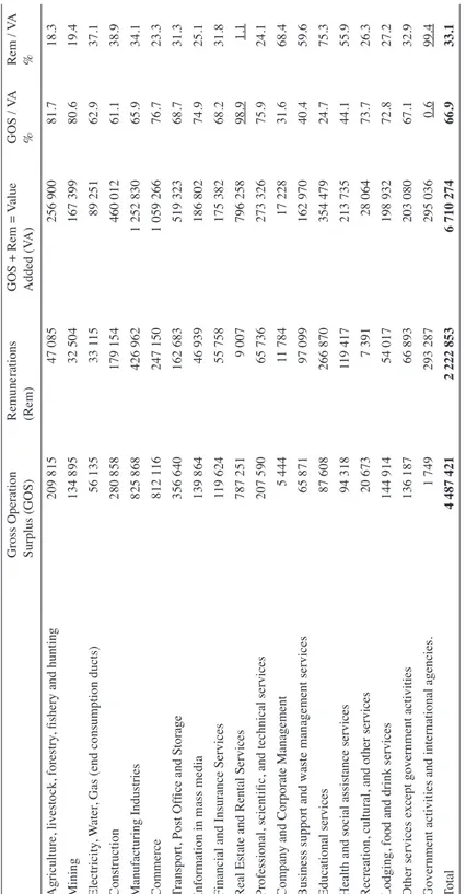
Basic study and characterization of the productive sectors Value Added and factorial participation
When the productive sectors of an economy are studied, the participation of the productive factors in obtaining the value added is one of the key points, given that from this it can be established if an Activity is relatively more or less intensive in the usage of capital or labor.
In Table 6 we calculated the sum of the payments to Capital and Labor for each Activity, what we call Value Added (VA), unlike the Gross Value Added (GVA) previously mentioned and which includes the Other taxes on production. In the last two columns of the Table we can observe the relative participations of the factors as percentages.
Altogether, the remunerations to the capital increase to twice what is paid for labor. Subsequently, there are two notorious extreme cases: that of the Real Estate sector, with a rather
high capital participation (98.9%), and that of the Government activities sector, with a rather
low participation (0.6%). For the rest of the sectors said participation is distributed, more or less, uniformly between 81.7% (Agriculture, livestock, ...) and 24.7% (Educational services).
In absolute terms, three sectors that repay the highest payments to the capital stand out: Manufacturing, Commerce, and Real Estate Services; these three sectors pay 54.1% of the GOS. Regarding Remunerations, four sectors stand out: Manufacturing, Commerce, Educational services and Government activities, paying 55.6% of the total Remunerations of the economy.
The most labor-intensive Activity, below the aforementioned extreme case, are Educational services (75.3%), followed by Corporate management (68.4%), though this is the smallest sector
and only generates 0.3% of the total VA. Furthermore, it clearly is a very specific and highly
specialized portion of the labor factor. The next two Activities with greater labor participation
Table 6 Factorial participation in the
Value
Added. (Millions of pesos 2003).
Gross Operation Surplus (GOS) Remunerations (Rem)
GOS + Rem =
Value Added (V A) GOS / V A % Rem / V A %
Agriculture, livestock, forestry
, fishery and hunting
209 815 47 085 256 900 81.7 18.3 Mining 134 895 32 504 167 399 80.6 19.4 Electricity , W ater
, Gas (end consumption ducts)
56 135 33 1 15 89 251 62.9 37.1 Construction 280 858 179 154 460 012 61.1 38.9 Manufacturing Industries 825 868 426 962
1 252 830
65.9 34.1 Commerce 812 1 16 247 150
1 059 266
76.7
23.3
Transport, Post Office and Storage
356 640
162 683
519 323
68.7
31.3
Information in mass media
139 864
46 939
186 802
74.9
25.1
Financial and Insurance Services
119 624
55 758
175 382
68.2
31.8
Real Estate and Rental Services
787 251
9 007
796 258
98.9
1.1
Professional, scientific, and technical services
207 590
65 736
273 326
75.9
24.1
Company and Corporate Management
5 444
11 784
17 228
31.6
68.4
Business support and waste management services
65 871 97 099 162 970 40.4 59.6 Educational services 87 608 266 870 354 479 24.7 75.3
Health and social assistance services
94 318
119 417
213 735
44.1
55.9
Recreation, cultural, and other services
20 673
7 391
28 064
73.7
26.3
Lodging, food and drink services
144 914
54 017
198 932
72.8
27.2
Other services except government activities
136 187
66 893
203 080
67.1
32.9
Government activities and international agencies.
1 749 293 287 295 036 0.6 99.4 Total
4 487 421
2 222 853
6 710 274
66.9
33.1
Source: Own elaboration with data from the Mexican System of National
The most capital-intensive Activity, below the aforementioned extreme case, is Agriculture, livestock... (81.7%), followed by Mining (80.6%), Commerce (76.7%), and Professional
services (75.9%).
Manufacturing and Commerce generate the highest VA, with a combined value of 34.5% of the total. Similarly, they also jointly pay 36.5% of the GOS, and 30.3% of the remunerations of the entire economy. The third sector that generates the highest VA is Real Estate, but the possibility for job creation here tends to be null.
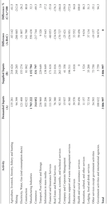
Inter-industrial exchanges
The participation that each industry or productive sector has in the contribution of inputs with regard to the rest of the industries for their processing and generation of goods and services, as well as the inputs it demands from the other sectors, comprise the most relevant interrelations to analyze the positioning of each sector and their importance in the network of
interrelations that define the interaction of all the industries among each other for the creation of
the economic wealth. Table 7 presents the inputs demanded by each sector from the others, the inputs it contributes, the absolute difference, and the difference as a percentage of the demand.
In this table, the negative differences mean that the demand is lower and thus there is a net positive supply; when the difference is positive, then the sector consumes more than it contributes to the others. Given that the sum of all the distributed inputs, stemming from the internal economy, is by necessity equal to the sum of all the demands for inputs, the sum of the differences is thus equal to zero.
Once more, in absolute terms, Manufacturing and Commerce are the sectors with greater demand and which contribute more inputs to the economy, but Manufacturing has a net demand of 32.3% (which could be interpreted as follows: for every 100 pesos of inputs it demands, it
supplies 67.7 pesos to the other sectors), whereas Commerce has a net supply of 69.3%, which means that for every 100 pesos it demands, it supplies 169.3 pesos to the rest of the economy.
The greatest supply rate of inputs is that of Business support and waste management services, which offer 472.8 pesos to the economy for every 100 pesos demanded, in second place we have Mining, supplying 312.8 pesos for every 100 demanded, and in third we have three service sectors: Real Estate, Professional, and Company Management, supplying 276.3,
284.8 and 259.5 pesos respectively for every 100 pesos they demand in inputs. Therefore, we can conclude that these five sectors seem to be the most necessary in the economy, in the sense
that they produce the inputs most required by the other productive sectors.
On the other extreme, we have the Activities that generate the greatest relative demands. It is immediately apparent that the Health sector, according to this account, has a null contribution to the rest of the economy, and presents only the necessary demand to provide the health services it generates. This poses a problem for this type of analysis, as health is a fundamental input. However, it is not treated as a direct input and as such is unaccounted, thus remaining as a sector that only consumes and does not contribute inputs to the rest of the economy. This, however, does not mean that it is not important, on the contrary, it can indicate that it has a high multiplying effect if the expenses in said sector increase; for example, a quality improvement policy for the public health services would immediately translate into 100% increases on the input demand it requires.
Table 7 Inter
-industrial exchanges. (Millions of pesos 2003).
Activity Demanded Inputs (A) Supplied Inputs (B) Differ ence (A-B=C) Differ ence % (C/A)*100
Agriculture, livestock, forestry
, fishery and hunting
135 281 218 424 -83 142 -61.5 Mining 94 399 295 285 -200 885 -212.8 Electricity , W ater
, Gas (end consumption ducts)
121 468 153 274 -31 807 -26.2 Construction 422 822 81 062 341 760 80.8 Manufacturing Industries
1 703 222
1 152 784
550 438 32.3 Commerce 314 052 531 797 -217 744 -69.3
Transport, Post Office and Storage
238 969
229 649
9 320
3.9
Information in mass media
101 206
138 849
-37 643
-37.2
Financial and Insurance Services
11
1 565
171 618
-60 053
-53.8
Real Estate and Rental Services
76 380
21
1 016
-134 636
-176.3
Professional, scientific, and technical services
92 393
263 120
-170 727
-184.8
Company and Corporate Management
15 937
41 358
-25 421
-159.5
Business support and waste management services
41 560 196 51 1 -154 951 -372.8 Educational services 39 570 6 018 33 552 84.8
Health and social assistance services
59 456
0
59 456
100.0
Recreation, cultural, and other services
11 157
1 524
9 634
86.3
Lodging, food and drink services
72 334
35 200
37 134
51.3
Other services except government activities
54 593
73 750
-19 157
-35.1
Government activities and international agencies.
100 632
5 759
94 874
94.3
Total
3 806 997
3 806 997
0
Source: Own elaboration with data from the Mexican System of National
Following this we have two service sectors, Education and Recreational, which supply 15.2 and 13.7 pesos, respectively, for every 100 they demand in inputs. We can say that these four sectors have a higher immediate carry-over effect and, therefore, can have greater multiplying effects.
Foreign trade
Another important indicator to evaluate the performance of the economy is given by the degree of foreign trade, that is, the measure in which goods and services are imported and exported, also known as the degree of integration with the global economy.
We begin with the imports, presenting the demand for national inputs in Table 8, followed by the demand of imports and, in the last column, the import of inputs as a ratio of the national inputs.
The first thing that calls our attention is that manufacturing, the most important sector of the economy, imports inputs for an equivalent of 61.9% of the national inputs, significantly above
the other sectors, which implies a high degree of integration (or dependence) of the global
economy. In the lower extreme, we have five sectors with input imports that, due to their own nature, represent less than 10% of the national inputs: Real Estate services (7.9%), Educational services (8.9%), Recreational services (8.5%), Lodging services (5.0%), and Government
activities (4.3%). For the rest of the Activities, the percentage varies, more or less uniformly, between 11.7% (Financial services) and 30.2% (Other services).
Table 8
Imported inputs. (Millions of pesos 2003).
Activity National
inputs (A)
Imported inputs (B)
Imported inputs as a percentage of the national inputs (B/A)*100
Agriculture, livestock, forestry, fishery and hunting 135 281 26 618 19.7
Mining 94 399 16 028 17.0
Electricity, Water, Gas (end consumption ducts) 121 468 22 675 18.7
Construction 422 822 68 481 16.2
Manufacturing Industries 1 703 222 1 054 394 61.9
Commerce 314 052 59 933 19.1
Transport, Post Office and Storage 238 969 53 314 22.3
Information in mass media 101 206 20 661 20.4
Financial and Insurance Services 111 565 13 035 11.7
Real Estate and Rental Services 76 380 5 999 7.9
Professional, scientific, and technical services 92 393 19 312 20.9
Company and Corporate Management 15 937 3 284 20.6
Business support and waste management services 41 560 8 978 21.6
Educational services 39 570 3 513 8.9
Health and social assistance services 59 456 11 197 18.8
Recreation, cultural, and other services 11 157 948 8.5
Lodging, food and drink services 72 334 3 597 5.0
Other services except government activities 54 593 16 503 30.2
Government activities and international agencies. 100 632 4 309 4.3
Total 3 806 997 1 412 778
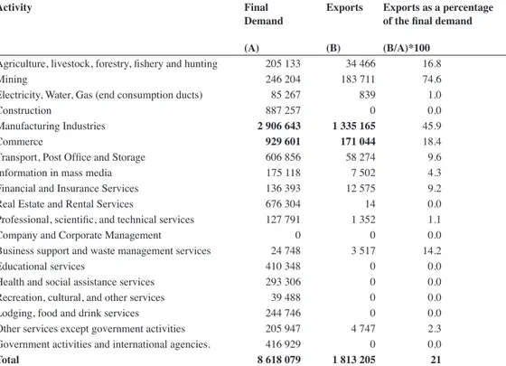
Let us now consider the exports. In Table 9, we present the total final demand per sector, the exports and, in the last column, the exports as a percentage of the total final demand. The
highest percentage observed, 74.6%, corresponds to Mining, explained by the presence of Pemex with its oil exports. In second place we have Manufacturing, with exports that increase
to close to half of its total net production of inputs (45.9%). In absolute terms, Manufacturing
is also the most important exporting sector of the economy; the exports of the previously seen Mining sector only represent 13.8% of the exports from Manufacturing. In third place we
have Commerce, which contributes 18.4% of its final consumption production. The rest of the Activities do not have significant exports.
Table 9. Exports. (Millions of pesos 2003).
Activity Final
Demand
(A)
Exports
(B)
Exports as a percentage of the final demand
(B/A)*100
Agriculture, livestock, forestry, fishery and hunting 205 133 34 466 16.8
Mining 246 204 183 711 74.6
Electricity, Water, Gas (end consumption ducts) 85 267 839 1.0
Construction 887 257 0 0.0
Manufacturing Industries 2 906 643 1 335 165 45.9
Commerce 929 601 171 044 18.4
Transport, Post Office and Storage 606 856 58 274 9.6
Information in mass media 175 118 7 502 4.3
Financial and Insurance Services 136 393 12 575 9.2
Real Estate and Rental Services 676 304 14 0.0
Professional, scientific, and technical services 127 791 1 352 1.1
Company and Corporate Management 0 0 0.0
Business support and waste management services 24 748 3 517 14.2
Educational services 410 348 0 0.0
Health and social assistance services 293 306 0 0.0
Recreation, cultural, and other services 39 488 0 0.0
Lodging, food and drink services 244 746 0 0.0
Other services except government activities 205 947 4 747 2.3 Government activities and international agencies. 416 929 0 0.0
Total 8 618 079 1 813 205 21
Source: Own elaboration with data from the Mexican System of National Accounts.
General Multipliers Matrix (GMM)
In this section, we used the SAM-Mx03ETD to carry out an identification exercise for
the accounts of our economy, based on the General Multipliers Matrix (GMM)—thus called
because it generalizes Leontief multipliers to a SAM—and using the definition of Rasmussen
indices.
Possibly, the most important utility—or at least the most exploited one of Leontief model—
therefore, the identification of those that have the most intense relations with the others (key sectors). In this manner, it could be argued that such sectors, should they receive significant
investments, would generate a higher growth for the economy.
Although various methods have been developed for the identification of key sectors, mainly
based on their “backward” and “forward” chaining (Iráizoz, 2006), and even when Rasmussen indices have received some critiques (Sonis et al., 1995, p. 234), in this work we calculated
the General Multipliers Matrix (GMM) and classified the accounts of our economy according to said indices—due to their broad use and because they comprise a first approximation to the
study of the structure of a real economy.
We will not go into detail regarding the specification of the model, as it is well known and many texts discuss it in detail (in particular, Miller and Blair, 2009, Ch. 6); it suffices to specify
that the general form of the model is:
y = M x (1)
Where y represents the income vector (equal to expense) of n=1, ..., N endogenous accounts;
M=(I–A)-1 is the multipliers matrix (equal to Leontief inverse when the endogenous accounts
are only the productive sectors); and x is an endogenous accounts vector (equal to the final
demand in Leontief model).
Each M element of column j is interpreted as the impact of an exogenous unitary increase directed to account j, over the income of each endogenous institution, so that the sum comprises the total multiplying effect.
Rasmussen indices simply compare the impact of each account or sector with the average impact, both by column (carry-over) and by row (dispersion), so that when a particular impact is higher to the average there is an index greater than one. Otherwise, the carry-over or impact
index per column is defined as:
(2)
Where is the average impact of the sector or account j over the other endogenous accounts, and N is the number of endogenous accounts or sectors. Similarly, the dispersion per
row of the index is defined as:
(3)
To carry out this exercise, we performed the follow modifications to the SAM, with the purpose of simplification. We eliminated the Societies account, making it so that the Capital
account directly does the distribution of the GOS. We also eliminated Private consumption, so that the Activities directly transfer the goods and services to the Households. Finally, we considered the Rest of the World and the Government as endogenous accounts along with the tax accounts.
Rasmussen indices that can be interpreted as a summary of the GMM, with the identification of
the 23 endogenous accounts of our economy.
According to these results, the productive factors have an above average impact, both in the carry-over and the dispersion, which is logical if we consider that all the productive sectors utilize them, and the income is generated from these. In the strategic sectors, the multiplier effect that the households have with the dispersion of their income is notable, which increases to 5.24, that is, each peso spent by the households generates a total dispersion of 5.24 pesos, an interesting result if a strengthening policy of the income of the households is considered. Table 10
Rasmussen carry-over and dispersion indices.
Account Carry-Over Index Dispersion Index Key Sectors
Capital 1.004 4.175
Labor 1.057 1.863
A6 1.061 1.173
Booster Sectors
A1 1.026 0.397
A7-A8 1.015 0.767
A9 1.034 0.384
A10 1.070 0.348
A11 1.094 0.884
A12 1.054 0.444
A14 1.056 0.300
A15 1.093 0.233
A16 1.054 0.221
A17 1.072 0.139
A18 1.084 0.349
A19 1.036 0.344
A20 1.084 0.117
Strategic Sectors
Households 0.949 5.239
Investment 0.879 1.491
A5 0.795 2.377
“Independent” Sectors
A2 0.586 0.341
A3 0.965 0.319
A4 0.992 0.949
A13 0.939 0.147
Source: Own elaboration. Final comments
detecting errors, making corrections, and adapting the matrix to specific research purposes. It
is worth noting that this SAM can be immediately extended to the next level of disaggregation
reported by the INEGI—which comprises 79 sectors of the NAICS—to carry out more detailed
analyses of the productive sectors.
Once specified, the SAM can be used to apply a broad range of multi-sectoral models
to the analysis of the Mexican economy, particularly the structural analysis and Applied General Equilibrium Models, with the advantage that the results can be replicated by different researchers and, consequently, can be discussed and validated or corrected.
Additionally, we carried out an analysis of the productive sectors, followed by the calculation of a generalized multipliers matrix that provides the total effects that a boost would have on
each productive sector. Finally, we identified the productive sectors based on Rasmussen
carry-over and dispersion indices.
According to other similar studies (Beltrán et al. 2016 and Sobarzo 2011), the classification of the productive sectors is consistent and comprises a useful guide for the economic policy
analysis. Especially, the identification of strategic sectors allows preventing bottlenecks that could hinder the growth of the economy, and that of booster sectors allows the identification of
Abbreviations used
Abbreviation Description
Households Households
Soc Societies
Gov Government
ISR Income Tax
CS Social Contributions
ISP Sales Tax
OIP Other Taxes on the Production
Savings Savings
Capital Capital
Labor Labor
A1 Agriculture, livestock, forestry use, fishery and hunting
A2 Mining
A3 Electricity, water, gas supply through ducts to the end consumer
A4 Construction
A5 Manufacturing
A6 Commerce
A7-A8 Transport, Post Office, and storage
A9 Mass media information
A10 Financial and insurance services
A11 Real estate and rental services of movable and intangible property
A12 Professional, scientific, and technical services
A13 Company and corporate management
A14 Business support and waste management services and cleanup services
A15 Educational services
A16 Health and social assistance services
A17 Entertainment, cultural, and sporting services, and other recreational services
A18 Temporary lodging and food and drink preparation services
A19 Other services except Government activities
A20 Government activities and international and extraterritorial agencies
ConsPriv Private Consumption
RoW Rest of the World
Appendix A.
SAM-Mx03ETD. Part 1. (Millions of pesos 2003).
Households Soc Gov ISR CS ISP OIP Investment
Households 3 513 249 113 241
Soc
Gov 396 616 147 621 388 413 310 631 4 617
ISR 226 509 170 107
CS
ISP 351 640
OIP
Savings 757 902 779 607 116 046
Capital Labor
A1 17 985
A2 62 493
A3 0
A4 29 886 029
A5 1 816 361 200
A6 0 87 736
A7-A8 0 20 670
A9 44 0
A10 30 083 0
A11 0 0
A12 12 089 0
A13 0 0
A14 0 0
A15 269 065 0
A16 162 309 0
A17 4 222 0
A18 0 0
A19 0 0
A20 412 665 0
ConsPriv 4 476 438
RoW 220 430 24 458 126 289 288 896
Total 6 032 919 4 487 421 1 247 897 396 616 147 621 388 413 310 631 1 729 627
Appendix A.
SAM-Mx03ETD. Part 2. (Millions of pesos 2003).
Capital Labor A1 A2 A3 A4 A5 A6
Households 2 239 206
Soc 4 487 421
Gov ISR
CS 3 127 2 159 2 199 11 898 28 355 16 413
ISP 1 512 1 001 2 309 3 335 10 518 521
OIP 118 260 503 640 1 771 10 108 11 213
Savings
Capital 209 815 134 895 56 135 280 858 825 868 812 116
Labor 47 085 32 504 33 115 179 154 426 962 247 150
A1 37 038 0 0 1 692 179 686 0
A2 76 5 917 1 852 12 077 275 010 0
A3 4 931 3 089 33 437 3 094 49 112 14 936
A4 924 353 579 62 592 6 448 511
A5 46 958 26 031 41 259 194 291 559 674 55 317
A6 22 588 12 130 20 023 65 355 286 675 28 748
A7-A8 8 670 6 176 9 523 23 783 104 148 12 911
A9 1 386 1 242 942 5 862 23 450 20 295
A10 5 241 14 635 3 806 5 682 19 789 42 033
A11 972 9 750 1 109 13 176 43 315 46 190
A12 5 051 4 104 1 832 18 648 54 371 75 465
A13 0 5 192 0 101 15 637 582
A14 6 1 875 2 691 8 461 53 308 10 511
A15 0 0 108 6 4 0
A16 0 0 0 0 0 0
A17 0 0 0 0 12 0
A18 40 1 108 660 2 838 12 620 77
A19 1 401 2 795 2 368 5 131 19 961 6 478
A20 0 0 1 278 31 0 0
ConsPriv
RoW 26 618 16 028 22 675 68 481 1 054 394 59 933
Total 4 487 421 2 239 206 423 557 541,489 238 541 968 320 4 059 427 1 461 397
Appendix A.
SAM-Mx03ETD. Part 3. (Millions of pesos 2003).
A7-A8 A9 A10 A11 A12 A13 A14 A15
Households Soc Gov ISR
CS 10 804 3 117 3 703 598 4 366 783 6 448 17 723
ISP 13 673 877 -52 181 570 56 241 70
OIP 422 1 304 4 377 7 903 943 4 070 1 061 1 012
Savings
Capital 356 640 139 864 119 624 787 251 207 590 5 444 65 871 87 608 Labor 162 683 46 939 55 758 9 007 65 736 11 784 97 099 266 870
A1 0 0 0 0 0 0 0 0
A2 7 1 0 222 4 0 4 0
A3 4 486 2 102 962 6 694 2 236 69 959 2 556
A4 1 063 73 510 3 304 64 293 232 1 109
A5 84 392 12 876 3 392 15 585 19 524 1 018 10 378 4 256
A6 34 666 6 765 1 815 5 796 10 283 291 4 518 2 196
A7-A8 22 680 7 356 4 052 2 974 5 602 794 2 298 1 529
A9 6 878 16 882 7 547 7 817 10 520 1 527 4 174 8 081
A10 16 224 5 339 35 163 2 980 1 355 3 007 784 507
A11 13 335 11 969 10 191 9 682 13 682 1 104 3 642 5 418
A12 16 176 8 800 17 204 4 157 15 058 5 254 7 521 6 500
A13 267 18 628 45 15 0 889 1 0
A14 16 597 7 607 24 242 15 418 9 731 517 5 641 4 995
A15 278 17 815 2 212 0 0 608
A16 0 0 0 0 0 0 0 0
A17 6 299 0 3 2 0 2 57
A18 4 492 399 1 391 304 2 005 956 935 891
A19 14 182 2 095 3 035 1 420 2 112 220 471 867
A20 3 241 0 1 199 7 0 0 0 0
ConsPriv
RoW 53 314 20 661 13 035 5 999 19 312 3 284 8 978 3 513
Total 836 505 313 968 308 011 887 319 390 911 41 358 221 259 416 366
Appendix A.
SAM-Mx03ETD. Part 4. (Millions of pesos 2003).
A16 A17 A18 A19 A20 ConsPriv RoW Total
Households 167 223 6 032 919
Soc 4 487 421
Gov 1 247 897
ISR 396 616
CS 7 931 491 3 587 4 442 19 477 147 621
ISP 350 30 329 436 815 388 413
OIP 637 322 1 167 642 2 418 310 631
Savings 76 071 1 729 627
Capital 94 318 20,673 144 914 136 187 1 749 4 487 421
Labor 119 417 7 391 54 017 66 893 293 287 16 353 2 239 206
A1 0 1 6 0 0 152 682 34 466 423 557
A2 0 1 114 0 0 0 183 711 541 489
A3 3 442 643 9 782 3 196 7 548 84 427 839 238 541
A4 422 29 853 94 1 607 1 199 0 968 320
A5 22 068 2 796 17 518 19 014 16 438 1 208 462 1 335 165 4 059 427
A6 8 749 976 6 116 8 301 5 804 670 821 171 044 1 461 397
A7-A8 3 196 467 2 756 3 323 7 411 527 912 58 274 836 505
A9 2 566 1 042 4 944 5 867 7 827 167 573 7 502 313 968
A10 367 296 4 582 1 302 8 526 93 735 12 575 308 011
A11 4 672 1 343 9 891 6 167 5 408 676 290 14 887 319
A12 2 478 1 030 3 832 3 771 11 868 114 350 1 352 390 911
A13 0 0 0 2 0 0 0 41 358
A14 8 573 1 829 9 098 2 937 12 473 21 231 3 517 221 259
A15 236 9 0 0 3 725 141 282 0 416 366
A16 0 0 0 0 0 130 997 0 293 306
A17 1 12 23 0 1 104 35 265 0 41 011
A18 893 82 134 248 5 127 244 746 0 279 946
A19 1 791 601 2 684 369 5 769 201 200 4 747 279 697
A20 0 0 0 3 0 4 263 0 422 688
ConsPriv 4 476 438
RoW 11 197 948 3 597 16 503 4 309 0 102 560 2 175 412
Total 293 306 41 011 279 946 279 697 422 688 4 476 438 2 175 412
Appendix B.
General Multipliers Matrix. Part 1.
Households Savings Capital Labor A1 A2 A3 A4 A5
Households 2.69 1.52 2.37 2.69 2.08 1.08 1.87 1.97 1.50
Savings 0.59 1.41 0.71 0.59 0.58 0.30 0.50 0.53 0.41
Capital 1.45 1.27 2.36 1.45 1.86 0.96 1.55 1.63 1.27
Labor 0.55 0.53 0.52 1.55 0.63 0.33 0.66 0.70 0.51
A1 0.13 0.11 0.12 0.13 1.21 0.06 0.11 0.11 0.13
A2 0.09 0.13 0.10 0.09 0.09 1.06 0.10 0.11 0.14
A3 0.08 0.06 0.07 0.08 0.08 0.04 1.23 0.07 0.07
A4 0.33 0.78 0.39 0.33 0.33 0.17 0.28 1.37 0.23
A5 0.99 0.99 0.95 0.99 0.97 0.49 0.98 1.03 1.78
A6 0.48 0.41 0.44 0.48 0.46 0.23 0.47 0.46 0.37
A7-A8 0.31 0.22 0.28 0.31 0.27 0.14 0.28 0.27 0.21
A9 0.12 0.08 0.10 0.12 0.10 0.05 0.09 0.10 0.08
A10 0.09 0.07 0.08 0.09 0.09 0.07 0.10 0.08 0.07
A11 0.36 0.23 0.33 0.36 0.29 0.17 0.27 0.30 0.23
A12 0.13 0.10 0.12 0.13 0.13 0.07 0.12 0.13 0.10
A13 0.01 0.01 0.01 0.01 0.01 0.02 0.01 0.01 0.01
A14 0.07 0.05 0.06 0.07 0.06 0.04 0.07 0.07 0.06
A15 0.06 0.04 0.06 0.06 0.05 0.03 0.05 0.05 0.04
A16 0.06 0.03 0.05 0.06 0.05 0.02 0.04 0.04 0.03
A17 0.02 0.01 0.01 0.02 0.01 0.01 0.01 0.01 0.01
A18 0.12 0.07 0.10 0.12 0.09 0.05 0.09 0.09 0.07
A19 0.11 0.07 0.10 0.11 0.09 0.05 0.09 0.09 0.07
A20 0.00 0.00 0.00 0.00 0.00 0.00 0.01 0.00 0.00
TMC 8.83 8.18 9.34 9.83 9.55 5.45 8.98 9.23 7.39
AMC 0.38 0.36 0.41 0.43 0.42 0.24 0.39 0.40 0.32
U.j 0.95 0.88 1.00 1.06 1.03 0.59 0.97 0.99 0.79
Appendix B.
General Multipliers Matrix. Part 2.
A6 A7-A8 A9 A10 A11 A12 A13 A14 A15
Households 2.21 2.09 2.11 2.20 2.30 2.19 1.90 2.26 2.42
Savings 0.62 0.57 0.58 0.60 0.68 0.61 0.49 0.57 0.58
Capital 1.94 1.76 1.83 1.84 2.26 1.92 1.43 1.66 1.60
Labor 0.69 0.71 0.69 0.76 0.54 0.69 0.78 0.96 1.17
A1 0.11 0.11 0.11 0.11 0.12 0.11 0.10 0.12 0.12
A2 0.09 0.09 0.09 0.09 0.10 0.09 0.08 0.09 0.09
A3 0.08 0.08 0.08 0.08 0.08 0.08 0.07 0.08 0.08
A4 0.34 0.32 0.33 0.33 0.38 0.34 0.28 0.32 0.33
A5 0.92 0.95 0.89 0.89 0.94 0.93 0.78 0.93 0.93
A6 1.44 0.44 0.42 0.42 0.44 0.44 0.37 0.44 0.45
A7-A8 0.27 1.28 0.28 0.28 0.28 0.28 0.25 0.28 0.28
A9 0.12 0.11 1.16 0.13 0.11 0.13 0.13 0.12 0.13
A10 0.11 0.10 0.10 1.21 0.09 0.08 0.15 0.09 0.09
A11 0.34 0.31 0.34 0.35 1.33 0.34 0.30 0.33 0.35
A12 0.17 0.13 0.15 0.18 0.12 1.15 0.24 0.15 0.14
A13 0.01 0.01 0.07 0.01 0.01 0.01 1.03 0.01 0.01
A14 0.07 0.08 0.09 0.15 0.08 0.09 0.08 1.09 0.07
A15 0.05 0.05 0.05 0.06 0.05 0.05 0.05 0.05 1.06
A16 0.05 0.05 0.05 0.05 0.05 0.05 0.04 0.05 0.05
A17 0.01 0.01 0.01 0.01 0.01 0.01 0.01 0.01 0.01
A18 0.10 0.10 0.10 0.10 0.10 0.10 0.11 0.10 0.11
A19 0.10 0.11 0.10 0.10 0.10 0.10 0.09 0.10 0.10
A20 0.00 0.01 0.00 0.01 0.00 0.00 0.00 0.00 0.00
TMC 9.87 9.45 9.62 9.95 10.18 9.81 8.73 9.82 10.17
AMC 0.43 0.41 0.42 0.43 0.44 0.43 0.38 0.43 0.44
U.j 1.06 1.02 1.03 1.07 1.09 1.05 0.94 1.06 1.09
Appendix B.
General Multipliers Matrix. Part 3.
A16 A17 A18 A19 A20 TMR AMR Ui.
Households 2.25 2.23 2.26 2.17 2.37 48.74 2.12 5.24
Savings 0.57 0.61 0.62 0.59 0.55 13.87 0.60 1.49
Capital 1.68 1.92 1.94 1.82 1.43 38.85 1.69 4.18
Labor 0.93 0.72 0.74 0.75 1.25 17.33 0.75 1.86
A1 0.12 0.12 0.12 0.11 0.12 3.70 0.16 0.40
A2 0.09 0.09 0.10 0.09 0.09 3.17 0.14 0.34
A3 0.09 0.09 0.11 0.08 0.10 2.97 0.13 0.32
A4 0.32 0.34 0.35 0.33 0.31 8.83 0.38 0.95
A5 0.96 0.97 0.97 0.94 0.95 22.11 0.96 2.38
A6 0.45 0.45 0.45 0.44 0.45 10.92 0.47 1.17
A7-A8 0.28 0.28 0.28 0.27 0.29 7.14 0.31 0.77
A9 0.11 0.13 0.12 0.12 0.13 3.57 0.16 0.38
A10 0.08 0.09 0.10 0.08 0.11 3.23 0.14 0.35
A11 0.33 0.34 0.35 0.32 0.34 8.22 0.36 0.88
A12 0.12 0.14 0.13 0.13 0.15 4.13 0.18 0.44
A13 0.01 0.01 0.01 0.01 0.01 1.37 0.06 0.15
A14 0.09 0.11 0.10 0.07 0.10 2.79 0.12 0.30
A15 0.05 0.05 0.05 0.05 0.06 2.17 0.09 0.23
A16 1.05 0.05 0.05 0.05 0.05 2.06 0.09 0.22
A17 0.01 1.01 0.01 0.01 0.02 1.29 0.06 0.14
A18 0.10 0.10 1.10 0.10 0.12 3.24 0.14 0.35
A19 0.10 0.11 0.11 1.09 0.11 3.20 0.14 0.34
A20 0.00 0.00 0.00 0.00 1.00 1.09 0.05 0.12
TMC 9.80 9.97 10.09 9.64 10.09 0.40
AMC 0.43 0.43 0.44 0.42 0.44
U.j 1.05 1.07 1.08 1.04 1.08 0.40
References
Aguayo, E. et al. (2009) Análisis de la generación y redistribución del ingreso en México a través de una Matriz de Contabilidad Social. Estudios Económicos, Número extraordinario.
Barbosa-Carrasco, I. et al. (2009) Matriz de Contabilidad Social 2004 para México. Agrociencia 43: 551-558. Beltrán, L. et al. (2015) Structural analysis of the mexican economy in 2008. 23rd International Input-Output
Con-ference. 22-26 June 2015, Mexico, Mexico City.
Defourney, J. and Thorbecke, E. (1984) Structural path analysis and multiplier decomposition within a social accoun
-ting framework. The Economic Journal, 94 (373). https://doi.org/10.2307/2232220
INEGI (2010a) Cuentas de bienes y servicios 2003-2008. Año base 2003. Tomos I y II. Segunda versión. México. INEGI (2010b) Cuentas por sectores institucionales 2003-2008. Año base 2003. Tomos I y II. Segunda versión.
México.
INEGI (2008) Matriz de insumo producto de México 2003. Clasificación SCIAN 2002. México.
Iráizoz, Belén (2006) ¿Es determinante el método en la identificación de los sectores clave de una economía? Una
aplicación al caso de las tablas input-output de Navarra(1). Estadística Española, 48 (163).
Leontief, W.W. (1936) Quantitative input and output relations in the economic systems of the United States. The
Re-view of Economic Statistics, 18 (3). https://doi.org/10.2307/1927837
Miller, R.E. And Blair, P.D. (2009) Input-output analysis: Foundations and extensions. Second edition. Cambridge
University Press, New York, USA.
Núñez, G. (2014) Macro matriz de contabilidad social de México para el año 2003. Econoquantum Revista de Eco-nomía y Negocios, 11 (2). https://doi.org/10.18381/eq.v11i2.2312
Sobarzo, H. (2011) Modelo de insumo-producto en formato de matriz de contabilidad social. Estimación de multipli-cadores e impactos para México, 2003. Economía Mexicana Nueva Época, 20 (2).