ADVERTIMENT. La consulta d’aquesta tesi queda condicionada a l’acceptació de les següents condicions d'ús: La difusió d’aquesta tesi per mitjà del servei TDX (www.tesisenxarxa.net) ha estat autoritzada pels titulars dels drets de propietat intel·lectual únicament per a usos privats emmarcats en activitats d’investigació i docència. No s’autoritza la seva reproducció amb finalitats de lucre ni la seva difusió i posada a disposició des d’un lloc aliè al servei TDX. No s’autoritza la presentació del seu contingut en una finestra o marc aliè a TDX (framing). Aquesta reserva de drets afecta tant al resum de presentació de la tesi com als seus continguts. En la utilització o cita de parts de la tesi és obligat indicar el nom de la persona autora.
ADVERTENCIA. La consulta de esta tesis queda condicionada a la aceptación de las siguientes condiciones de uso: La difusión de esta tesis por medio del servicio TDR (www.tesisenred.net) ha sido autorizada por los titulares de los derechos de propiedad intelectual únicamente para usos privados enmarcados en actividades de investigación y docencia. No se autoriza su reproducción con finalidades de lucro ni su difusión y puesta a disposición desde un sitio ajeno al servicio TDR. No se autoriza la presentación de su contenido en una ventana o marco ajeno a TDR (framing). Esta reserva de derechos afecta tanto al resumen de presentación de la tesis como a sus contenidos. En la utilización o cita de partes de la tesis es obligado indicar el nombre de la persona autora.
Geochemical kinetics during
CO2
sequestration: the reactivity
of the Hontomín
caprock
and the hydration of
MgO
Gabriela Dávila Ordoñez
PhD Thesis
Department of Geotechnical Engineering and Geo-Sciences (ETCG) Technical University of Catalonia (UPC)
Supervisors:
Dr. Jordi Cama Dra. Linda Luquot Dr. Josep M. Soler
Acta de calificación de tesis doctoral Curso académico:
Nombre y apellidos: MARIA GABRIELA DÁVILA ORDOÑEZ
Programa de doctorado:
Unidad estructural responsable del programa
Resolución del Tribunal
Reunido el Tribunal designado a tal efecto, el doctorando / la doctoranda expone el tema de la su tesis doctoral titulada
____________________________________________________________________________________
__________________________________________________________________________________________.
Acabada la lectura y después de dar respuesta a las cuestiones formuladas por los miembros titulares del tribunal, éste
otorga la calificación:
NO APTO APROBADO NOTABLE SOBRESALIENTE
(Nombre, apellidos y firma)
Presidente/a
(Nombre, apellidos y firma)
Secretario/a
(Nombre, apellidos y firma)
Vocal
(Nombre, apellidos y firma)
Vocal
(Nombre, apellidos y firma)
Vocal
______________________, _______ de __________________ de _______________
El resultado del escrutinio de los votos emitidos por los miembros titulares del tribunal, efectuado por la Escuela de
Doctorado, a instancia de la Comisión de Doctorado de la UPC, otorga la MENCIÓN CUM LAUDE:
SÍ NO
(Nombre, apellidos y firma)
Presidente de la Comisión Permanente de la Escuela de Doctorado
(Nombre, apellidos y firma)
Secretario de la Comisión Permanente de la Escuela de Doctorado
TECHNICAL UNIVERSITY OF CATALONIA (UPC)
DEPARTMENT OF GEOTECHNICAL ENGINEERING AND GEO-SCIENCES (ETCG)
Geochemical kinetics during
CO2
sequestration: the reactivity
of the Hontomín
caprock
and the hydration of
MgO
Thesis presented by
Gabriela Dávila Ordoñez
Work conducted in the Institute of Environmental Assessment and Water Research (IDAEA-CSIC) under the supervision of
Dr. Jordi Cama i Robert
Institute of Environmental Assessment and Water Research (IDAEA), CSIC
Dra. Linda Luquot
Institute of Environmental Assessment and Water Research (IDAEA), CSIC
Dr. Josep M. Soler
Institute of Environmental Assessment and Water Research (IDAEA), CSIC
Barcelona, November 2015
Abstract
A test site for CO2 geological storage is situated in Hontomín (Burgos, Northern Spain) with a reservoir rock that is mainly composed of limestone. The reservoir rock is a deep saline aquifer, which contains a NaCl- and sulfate-rich groundwater in equilibrium with calcite and gypsum, and is covered by a very low permeability formation composed of marls, marly limestone and bituminous shales which acts as a caprock. During and after CO2 injection, since the resident groundwater contains sulfate, the resulting CO2-rich acid solution may give rise to the dissolution of calcite (carbonate mineral) and albite, illite and clinochlore (Si-bearing minerals), and secondary sulfate-rich mineral precipitation (gypsum or anhydrite) together with that of Si-bearing minerals (clay and zeolites) may occur. These reactions that may imply changes in the porosity, permeability and pore structure of the rock could alter the CO2 seal capacity of the caprock.
Therefore, performing reliable experiments and reactive transport modeling to gain knowledge about the overall process of gypsum precipitation at the expense of calcite dissolution in CO2-rich solutions and its implications for the hydrodynamic properties of the caprock is necessary.
A first aim of this thesis is to better understand these coupled reactions by assessing the effect that
P, pCO2, T, mineralogy, acidity and solution saturation state exert on these reactions. To this end, flow-through experiments with illite powder samples and flow-through experiments and columns filled with crushed marly limestone, bituminous black shale and marl are conducted under different P–pCO2 conditions (atmospheric: 1–10-3.5, subcritical: 10–10 bar and supercritical: 150– 37 bar), T (25 and 60 °C) and input solution compositions (undersaturated and gypsum-equilibrated solutions). The CrunchFlow numerical code was used to perform 1D reactive transport simulations of the experiments to evaluate mineral reaction rates in the system and quantify the porosity variation along the columns.
A second aim of this PhD study is to evaluate the interaction between the Hontomín marl and CO2-rich sulfate solutions under supercritical CO2 conditions (PTotal = 150 bar, pCO2 = 61 bar and
effect of the flow rate (0.2, 1 and 60 mL h-1) on fracture permeability. Major dissolution of calcite (S-free and S-rich solutions) and precipitation of gypsum (S-rich solution) together with minor dissolution of the silicate minerals contributed to the formation of an altered skeleton-like zone (mainly made up of unreacted clays) along the fracture walls. Dissolution patterns changed from face dissolution to wormhole formation and uniform dissolution with increasing Peclet numbers.
In S-free experiments, fracture permeability did not significantly change regardless of the flow rate
despite the fact that a large amount of calcite dissolved. In S-rich solution experiments, fracture permeability decreased under slow flow rates (0.2 and 1 mL h-1) because of gypsum precipitation that sealed the fracture. At the highest flow rate (60 mL h-1), fracture permeability increased because calcite dissolution predominated over gypsum precipitation.
2D reactive transport models were used to interpret the results of the experiments (not at 60 mL h-1) and reproduced the variation in the outflow composition with time and the observed width of the alteration zone along the fractures. The good match was achieved by using an initial Deff value
from 3 × 10-13 m2 s-1 to 1 × 10-13 m2 s-1 under slow flow rate and by increasing it by a factor of 20 (6 × 10-12 m2 s-1) in the rock matrix under fast flow rate. Additionally, a slight change in the calcite reactive surface areas contributed to the fit of the model to the experimental data.
The modeling reproduced the large dissolution of calcite, minor dissolution of clinochlore and gypsum precipitation. Calcite dissolution was favored by increasing the flow rate and gypsum precipitation was large under 1 mL h-1 flow conditions. Minor precipitation of dolomite, kaolinite and two zeolites (mesolite and stilbite) along the altered zone was likely. The magnitude of these reactions is consistent with the measured increase in porosity over the altered zone, which was fairly reproduced.
The third aim is to study caustic magnesia (MgO) as an alternative to Portland cement, not only
(CaMg(CO3)2), nesquehonite (MgCO3·3(H2O)), hydromagnesite (Mg5(CO3)4(OH)2·4(H2O)) and magnesite (MgCO3)). Different T and pCO2 conditions will determine the formation of these
carbonates. The molar volumes of the implicated minerals (cm3 mol-1) [(Mg(OH)2 (24.63), CaCO3 (36.93), MgCO3 (28.02), CaMg(CO3)2 (64.37), Mg5(CO3)4(OH)2·4(H2O) (208.08), MgCO3·3(H2O) (75.47)], with large molar volumes for the secondary phases, favor a potential decrease in porosity and hence the sealing of cracks in cement structures, preventing CO2 leakage.
As a preliminary study for the potential use of MgO as an alternative to Portland cement in injection wells, MgO carbonation has been studied by means of batch experiments under subcritic (pCO2 of 10 and 50 bar and T of 25, 70 and 90 °C) and supercritic (pCO2 of 74 bar and T of 70 and 90 °C) CO2 conditions.
Magnesium oxide reacts with CO2-containing and Ca-rich water nearly equilibrated with respect to calcite. MgO quickly hydrates to brucite which dissolves causing the precipitation of magnesium carbonate phases. Precipitation of these secondary phases (magnesite and/or metastable phases such as nesquehonite or hydromagnesite depends on pCO2, temperature and solid/water content. In a constant solid/water ratio, the precipitation of the non-hydrated Mg carbonate is favored by increasing temperature and pCO2.
Resum
Un lloc de prova per a l'emmagatzematge geològic de CO2 es troba en Hontomín (Burgos, nord d'Espanya) on la roca reservori es compon principalment de roca calcària. La roca reservori és un aqüífer salí profund, que conté una aigua subterrània rica en NaCl- i sulfat en equilibri amb calcita i guix, i està coberta per una formació de molt baixa permeabilitat composta de margues, calcàries margoses i lutites bituminoses, que actua com a roca segell. Durant i després de la injecció de CO2, com que l'aigua subterrània resident conté sulfat, la solució àcida resultant rica en CO2 pot donar lloc a la dissolució de calcita, albita, illita i clinoclor (minerals rics en Si), i precipitació de minerals de sulfat (guix o anhidrita), juntament amb la de minerals rics en Si (argiles i zeolites). Aquestes reaccions que poden implicar canvis en l'estructura de la porositat, la permeabilitat i dels porus de la roca podrien variar la capacitat de segellat de CO2 de la roca segell.
Per tant, és necessària la realització d'experiments fiables i la modelització del transport reactiu per adquirir un millor coneixement sobre el procés general de la precipitació de guix, a costa de la dissolució de calcita en solucions riques en CO2 i les seves implicacions per a les propietats hidrodinàmiques de la roca segell.
Un primer objectiu d'aquesta tesi és poder comprendre aquestes reaccions acoblades mitjançant
Un segon objectiu d'aquest estudi de doctorat és avaluar la interacció entre la marga d’Hontomín i solucions de sulfat riques en CO2 sota condicions de CO2 supercrític (PTotal = 150 bar, pCO2 = 61 bar i T = 60 °C). Es van realitzar experiments de percolació usant testimonis fracturats artificialment per dilucidar (i) el paper de la composició de les solucions injectades (solucions sense S i solucions riques en S), (ii) l'efecte de la velocitat de flux (0.2, 1 i 60 ml h-1) en la permeabilitat de la fractura. Una major dissolució de calcita (ambdós solucions), i la precipitació de guix (solució rica en S), juntament amb una menor dissolució dels minerals de silici, van contribuir a la formació d'una zona alterada (constituïda principalment d'argiles gairebé sense reaccionar) al llarg de les parets de la fractura. Els patrons de dissolució van canviar de tipus “dissolució d’entrada” (face dissolution) a “forat de cuc” (wormhole) i “dissolució uniforme” (uniform dissolution) amb l’increment del número de Peclet.
En els experiments en solucion sense S, la permeabilitat de la fractura no va canviar significativament, independentment de la velocitat de flux i de la dissolució significativa de calcita. En els experiments en solució rica en S, la permeabilitat de la fractura es va reduir a velocitat baixes de flux (0,2 i 1 mL h-1) a causa de la precipitació de guix que va segellar la fractura. A la velocitat de flux més alta (60 ml h-1), la permeabilitat de la fractura va augmentar a causa de la dissolució de calcita que va predominar sobre la precipitació de guix.
Es van realitzar models 2D de transport reactiu per interpretar els resultats dels experiments (no els de 60 ml h-1) que van reproduir la variació en la composició de flux de sortida amb el temps i l'amplada de la zona d'alteració observada al llarg de les fractures. Es va aconseguir un bon resultat amb l’ús d'un valor inicial de Deff de 3 × 10-13 m2 s-1 fins a 1 × 10-13 m2 s-1 a cabal lent i
amb un valor Deff vint vegades major (6 × 10-12 m2 s-1) a cabal ràpid. A més a més, un lleuger
canvi en les àrees de superfície reactiva de al calcita va contribuir a l'ajust del model amb les dades experimentals.
alterada. La magnitud d'aquestes reaccions és consistent amb l'augment de porositat mesurat a la zona alterada.
El tercer objectiu és l'estudi de la magnèsia càustica (MgO) com una alternativa al ciment Portland, no només per ser utilitzat en l'espai entre el revestiment del pou i la roca, sinó també per segellar les fractures de roca. El procés de carbonatació del MgO es considera que passa quan el MgO s’hidrata ràpidament per formar brucita (Mg (OH)2). Quan la brucita es dissol en una solució rica en Ca i saturada en CO2, la solució se sobresatura respecte dels carbonates de Ca i/o de Mg (per exemple, dolomita (CaMg (CO3)2), nesquehonita (MgCO3·3 (H2O)), hidromagnesita (Mg5(CO3)4(OH) 2·4 (H2O)) i magnesita (MgCO3)). Diferents condicions de T i pCO2 determinen la formació d'aquests carbonats. Els volums molars dels minerals implicats (cm3mol-1) [(Mg(OH)2 (24.63), CaCO3 (36.93), MgCO3 (28.02), CaMg (CO3)2 (64.37), Mg5(CO3)4(OH)2·4(H2O) (208.08), MgCO3·3(H2O) (75.47)], amb volums molars més grans per a les fases secundàries, juguen a favor d'una possible disminució de la porositat, i per tant, del segellat d'esquerdes en les estructures de ciment, impedint les fuites de CO2 .
Com a estudi preliminar per a l'ús potencial de MgO com alternativa al ciment Portland en els pous d'injecció, s’ha estudiat la carbonatació del MgO per mitjà d'experiments en condicions de CO2 subcrític (pCO2 de 10 i 50 bar i T de 25, 70 i 90 °C) i CO2 supercrític (pCO2 de 74 bar i T de 70 i 90 °C).
L'òxid de magnesi reacciona amb l'aigua rica en CO2 dissolt i Ca, gairebé equilibrada amb calcita. El MgO s’hidrata ràpidament a brucita que es dissol provocant la precipitació de fases carbonatades de magnesi. La precipitació d'aquestes fases secundàries (magnesita i/o fases metastables com ara nesquehonita o hidromagnesita depèn de la pCO2, la temperatura i el contingut de sòlids/aigua. En una relació sòlid/aigua constant, la precipitació del carbonat de Mg no hidratat es veu afavorida per l'augment de la temperatura i de la pCO2.
Resumen
Una planta piloto para el almacenamiento geológico de CO2 se encuentra ubicada en Hontomín (Burgos, norte de España). Hontomín es un yacimiento que se compone principalmente de roca caliza. El reservorio es un acuífero salino profundo, que contiene un agua subterránea rica en NaCl- y sulfato, dicha agua se encuentra en equilibrio con calcita y yeso. Este reservorio está cubierto por una formación que tiene muy baja permeabilidad y está constituida principalmente de margas, calizas margosas y lutitas bituminosas, las cuales actúan como roca sello. Durante y después de la inyección de CO2, ya que el agua subterránea residente contiene sulfato, la solución acida rica en CO2 resultante da lugar a la disolución de calcita (minerales de carbonato) y de albita, illita y Clinochloro (minerales ricos en Si), así como la precipitación de minerales ricos en sulfato (e.g. yeso o anhidrita) y en silicio (e.g. arcilla y zeolitas). Estas reacciones que se producen pueden implicar cambios en la estructura (porosidad), la permeabilidad y en los poros de la roca los cuales podrían variar la capacidad de sellado de la roca. Por lo tanto es indispensable realizar experimentos de laboratorio y modelizar mediante transporte reactivo con el fin de adquirir los conocimientos sobre el proceso de la precipitación de yeso, a expensas de la disolución de la calcita en soluciones ricas en CO2 y las implicaciones que tiene en las propiedades hidrodinámicas de la roca sello.
Un primer objetivo de esta tesis se basa en comprender el comportamiento de dichas reacciones
Un segundo objetivo de este estudio de doctorado es evaluar la interacción entre la marga de Hontomín y soluciones ricas en sulfato y CO2 bajo condiciones de CO2 supercrítico (PTotal = 150
bar, pCO2 = 61 bar y T = 60 °C). Para dicho estudio se realizaron experimentos de percolación de flujo a través de columnas usando muestras de cores fracturados artificialmente con el fin de dilucidar (i) el papel que juega la composición de las soluciones inyectadas (soluciones ricas y libres en sulfato), y (ii) el efecto de la velocidad de flujo (0.2, 1 y 60 ml h-1) que ejercen sobre la permeabilidad de la fractura. La disolución de calcita (en ambas soluciones de entrada), y la precipitación de yeso (en la solución rica en sulfato) junto a la disolución de los minerales de silicato (en menor proporción), contribuyen a la formación de una zona esquelética alterada (principalmente compuesta por arcillas no reaccionadas) a lo largo de las paredes de la fractura. Un crecimiento en el número de Pe rige los cambios en los patrones de disolución (disolución de cara, disolución de agujero y disolución uniforme).
En los experimentos realizados con el agua sin sulfato, la permeabilidad de la fractura no cambió significativamente, independientemente de la velocidad de flujo a pesar del hecho de que una gran cantidad de calcita se disolvió. Contrariamente, en los experimentos realizados con el agua rica en sulfato, la permeabilidad de la fractura se redujo en presencia de flujos lentos (0.2 y 1 mL h-1), esto se debe a que la precipitación de yeso se encarga de sellar la fractura. A velocidad de flujo alto (60 ml h-1), la permeabilidad de la fractura aumentó debido a que la disolución de la calcita predominó sobre la precipitación de yeso.
Se utilizaron modelos 2D de transporte reactivo para interpretar los resultados de los experimentos (excepto a 60 mL h-1) y se reproduce la variación en la concentración de salida con el tiempo, así como la anchura observada de la zona de alteración a lo largo de las fracturas. El mejor ajuste encontrado fue obtenido mediante el uso de un valor de Deff inicial de 3 × 10-13 m2 s-1 para el
caudal lento y 1 × 10-13 m2 s-1 para el caudal medio, teniendo que aumentar por un factor de 20 (6 × 10-12 m2 s-1) en la matriz de roca a caudal rápido. Conjuntamente con un ligero cambio en el área reactiva de la calcita contribuyó al ajuste del modelo a los datos experimentales.
de la velocidad de flujo y la precipitación de yeso. La precipitación en menor proporción de dolomita, caolín y zeolitas (mésolite y estilbita) a lo largo de la zona alterada fue calculada mediante las simulaciones. La magnitud de estas reacciones es consistente con el aumento en la porosidad medida en la zona alterada.
El tercer objetivo es el estudio de magnesia cáustica (MgO) como una alternativa al cemento Portland, no sólo para ser utilizado en el espacio entre el revestimiento del pozo y la roca, sino también para sellar las fracturas de roca (lechada). El proceso general de carbonatación del MgO se considera que ocurra cuando MgO se hidrata rápidamente para formar brucita (Mg (OH)2). Cuando la brucita se disuelve en una solución rica en Ca y CO2-saturado, la solución se supersatura con respecto a los carbonatos de Ca y/o Mg (e.g. dolomita (CaMg (CO3)2), nesquehonita (MgCO3·3(H2O)), hidromagnesita (Mg5(CO3)4(OH)2·4(H2O)) y magnesita (MgCO3)). Diferentes condiciones de pCO2 y T determinarán la formación de estos carbonatos. Los grandes volúmenes molares de las fases secundarias (cm3 mol-1) [MgCO
3 (28.02), CaMg (CO3)2 (64.37), Mg5(CO3)4(OH)2·4(H2O) (208.08), MgCO3·3(H2O) (75.47)], con respecto a los primarios [(Mg(OH)2 (24.63), CaCO3 (36.93)], favorecen una posible disminución de la porosidad y por lo tanto, el sellado de grietas en estructuras de cemento así como la prevención de fugas de CO2.
Un estudio preliminar para el uso potencial MgO como una alternativa al cemento Portland en pozos de inyección, la carbonatación del MgO ha sido estudiado por medio de experimentos por lotes bajo condiciones de CO2 subcrítico (pCO2 de 10 y 50 bar y T de 25, 70 y 90 ° C) y supercrítico (pCO2 de 74 bar y T de 70 y 90 ° C).
Acknowledgements
The work presented in this Ph.D. study contains the results collected through six years of research in the Groundwater Hydrology Group (UPC-CSIC). For this reason, the list of people who has contributed and supported it cannot be exhaustive.
I want to thank my supervisor Jordi Cama whose encouragement, guidance, support and trust, enabled me to obtain the results achieved. I also thank him for teaching me how to carry out laboratory experiments and interpret and quantify the results. I am in debt with him and hope to keep our collaboration up in the near future. It has been a honor to be his Ph.D. student.
Thanks are due to my supervisor Dr. Josep M. Soler for teaching me how to use the CrunchFlow reactive transport code and model and analyze properly the experimental results. Many times after feeling “I’ve tried all”, he looked at the files and came out with a new idea.
I would like to thank my supervisor Dr. Linda Luquot for her constant help in every kind of practical and theoretical problem, at any moment, day or night. Thanks also for your special support over long nights at the ESRF Synchrotron (Grenoble) and during the hard weeks working with the ICARE apparatus at the University of Montpellier.
I am heartily thankful to Dr. Jesús Carrera to give me the chance to join this group.
I am very grateful to Javier Gargía-Veigas and Maite Romero from the Scientific and Technical Services of the University of Barcelona (CCiT-UB) for their technical assistance in the SEM-EDX and ICP-AES analyses, Natàlia Moreno (IDAEA-CSIC) for her help in the XRD analyses and Elisenda Seguí (CCiT-UB) for her assistance in the X-ray fluorescence analyses.
I also place on record, my sincere thanks to Dr. Charlotte Garing (Stanford University) and Dr. Philippe Gouze (CNRS-Montpellier) for their constructive comments that have improved the quality of this Ph.D. manuscript.
Many thanks to Dr. Anna Russian (UPC) for her unconditional help and support over these years of research. My time at the IDAEA was largely enjoyable in a large part thanks to my friends, who have become part of my life: Maria García, Francesco Offeddu, Cristina Valhondo, Yoar Cabeza, Victor Bezos, Ester Torres and Eike Thaysen (and baby Magnus). They have helped making life easier and funnier at the institute. I also want to thank all the IDAEA team for having good time.
Table of contents
Chapter I
Introduction ... 1
1.1 CO2 emissions ... 3
1.2 Geological Storage ... 5
1.3 CO2 leakage through caprock and wells ... 6
1.3.1 Caprock ... 7
1.3.2 Well ... 8
1.4 Motivation ... 10
1.5 Thesis outline ... 13
Chapter II
Materials and Methods... 152.1.Experimental methodology ... 17
2.1.1 Analytical methods ... 17
2.1.2 Sample characterization ... 19
2.1.3 Injected solutions ... 27
2.1.3.1 Flow-through experiments ... 27
2.1.3.2 Column experiments ... 27
2.1.3.3 Percolation experiments ... 28
2.1.3.4 Batch experiments ... 28
2.1.4 Experimental Setup and Methodology ... 30
2.1.4.1 Flow-through experimental setup (atm-CO2; pCO2 = 10-3.5 bar) ... 30
2.1.4.2 Column experimental setup (atm-CO2; pCO2 = 10-3.5 bar) ... 31
2.1.4.3 Column experimental setup (subc.-CO2 ; pCO2 = 10 bar) ... 32
2.1.4.4 Column and percolation experimental setups (supc.-CO2; pCO2 = 150 bar) ... 34
2.1.4.5 Batch experimental setup (pCO2 ≥ 10 bar) ... 36
2.2.Calculations ... 37
2.2.1 Calculation of the illite dissolution rate ... 37
2.2.2 Calculation of parameters used in the reactive transport modeling ... 37
2.2.3 Mass balance calculations ... 39
2.2.5 Calculation of saturation index ... 43
2.3.Reactive transport modeling ... 45
2.3.1 Description of the reactive transport code ... 45
2.3.2 One and zero-dimensional model (Chapter III and V: flow-through, column and batch experiments) ... 47
2.3.2.1 Numerical discretization ... 48
2.3.2.2 Rock and solution compositions ... 48
2.3.2.3 Flow and transport properties ... 51
2.3.2.4 Thermodynamic and kinetic data ... 51
2.3.2.5 Reaction rates ... 52
2.3.3 Two- dimensional model (Chapter IV: percolation experiments) ... 54
2.3.3.1 Numerical discretization ... 54
2.3.3.2 Rock and solution compositions ... 55
2.3.3.3 Flow and transport properties ... 58
2.3.3.4 Thermodynamic and kinetic data ... 58
2.3.3.5 Reaction rates ... 58
Chapter III
Dissolution of illite and marl caprocks under subcritical and supercritical CO2 conditions at 25 and 60 °C: flow-through, column experiments and 1D reactive transport modeling ... 593.1 Introduction ... 61
3.2 Flow-through experiments ... 62
3.2.1 Illite ... 62
3.2.2 Marly limestone ... 65
3.3 Column experiments ... 69
3.3.1 S-free solution experiments; pCO2 = 10-3.5 bar ... 71
3.3.2 S-rich solution experiments; pCO2 = 10-3.5 bar ... 75
3.3.3 T effect on marl reactivity; pCO2 = 10 bar ... 80
3.3.4 pCO2 effect on marl reactivity ... 85
3.4 Summary and conclusions ... 90
4.1.Introduction ... 95 4.2.Results ... 95 4.2.1.Experimental results... 95 4.2.1.1 Dissolution and precipitation processes ... 96 4.2.1.1.1 Output concentrations ... 96 4.2.1.1.2 Influence of the flow rate ... 100 4.2.1.2 Alteration of the rock ... 105 4.2.1.3 Dissolution patterns ... 108 4.2.1.4 Fracture permeability ... 110 4.2.2.Modeling results ... 112 4.2.2.1 Dissolution and precipitation processes ... 112 4.2.2.1.1 S-rich injected solution ... 112 4.2.2.1.2 S-free injected solution ... 118 4.2.2.2 Mineral dissolution and precipitation rates ... 119 4.2.2.2.1 Primary minerals ... 119 4.2.2.2.2 Secondary minerals... 121 4.2.2.3 Variation in mineral volume ... 122 4.2.2.4 Variation in porosity ... 126 4.3.Summary and conclusion ... 127
Chapter V
Efficiency of magnesium hydroxide as engineering seal in the geological sequestration of CO2 .... 131
5.1 Introduction ... 133 5.2 Results ... 133 5.2.1 Experimental results... 133 5.2.2 Modeling results ... 137 5.2.3 Application case: borehole-cement-reservoir rock interface ... 145 5.3 Summary and conclusions ... 149
Chapter VI
Conclusions ... 151
Appendixes ... 161
List of figures
Figure 1.1 World CO2 emissions from fossil fuels used by country. Data from International Energy Annual
2006, Energy information Administration. (CO2CRC, 2015) ... 4 Figure 1.2 GHG trends and projections 1990-2020 of the CO2 equivalent. Total emissions by the European
Environmental Agency (EEA, 2012)... 4
Figure 1.3 Diagrammatic illustration of geological carbon storage. CO2 from concentrated sources is
separated from other gasses compressed and injected into porous geological strata at depths >800 m where it is in a dense or supercritical phase. The CO2 is lighter than formation brines, rises and is trapped by
impermeable strata. The risks are that the light CO2 will exploit faults or other permeable pathways to
escape upwards and acid CO2-charged brines might corrode the caprocks or fault zones (Kapman et al.,
2014) ... 6
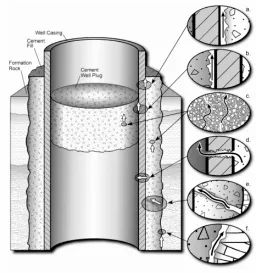
Figure 1.4 Diagrammatic representation of possible leakage pathways through an abandoned well. a) Between casing and cement; b) between cement plug and casing; c) through the cement pore space; d) through casing; e) through fractures in cement; and f ) between cement and rock (Gasda et al. 2004) ... 9
Figure 1.5 Scheme of the stratigraphic column of the Hontomín site (GEOMODELS, University of Barcelona). Depth of CO2 injection in the reservoir is between 1414-1530 m ... 12 Figure 2.1 Picture of caprock samples from the Hontomín reservoir: marly limestone, bituminous black shale and marl. Inset images show powder (< 63 m), crushed sample (1-2 m) and core (18 mm in length and 9 mm in diameter) ... 20
Figure 2.2SEM images from the initial S4.3 marl sample. (a) grain size (between 1-2 mm) and (b) surface of the grain. (c) EDS spectrum of the elements present in the sample ... 23
Figure 2.3 Preparation of the fractured core samples of the S4.3 marl: a) cored, b) clipped, c) fractured and d) sealed ... 24
Figure 2.4 ESEM images of the unreacted S4.3 marl thin section with local spectrum analysis ... 25
Figure 2.5 Schematics of ESEM thin section and XMT sections of the core sample (a), ESEM image showing the initial fracture aperture of the exp. 23 (b) and 3D microtomography image of the core sample (c) ... 25
Figure 2.6 SEM images from the initial MgO sample; a) different grains and b) brucite ... 26
Figure 2.8 Scheme of the experimental setup used in the column experiments under atmospheric conditions ... 32 Figure 2.9 Scheme that shows the experimental setup used to perform column experiments under 10 bar of pCO2 ... 33 Figure 2.10 Schemes showing: a) the ICARE Lab CSS I experimental setup and b) the ICARE Lab CSS II experimental setup. CO2 is added from a liquid CO2 reservoir ... 35 Figure 2.11 Photography (a) and scheme (b) of the experimental setups to perform batch experiments under different PTotal, pCO2 and T conditions... 36 Figure 2.12 Schemes showing: the spatial discretization corresponding to the fractured marl cores a) cylindrical coordinates and b) rectangular coordinates, and c) mesh distribution along the core sample .. 55
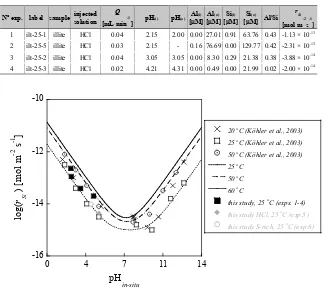
Figure 3.1 Temporal variation of output Si and Al concentrations (a) and pH (b) during the illite du Puy dissolution experiments at atmospheric pressure and 25 °C. Si =○ and Al =●; exp.1 = ○, exp 2 = ◊, exp. 3 = □ and exp4 = Δ. Black and gray color indicates input and output solution, respectively. ... 62
Figure 3.2 Rates of illite dissolution as a function of pH and temperature: 20‚ 25 and 50 °C. The open symbols represent experimental rates of Köhler et al. (2003) and solid lines the calculated rates using the parameters from Oelkers et al. (2001). Black and gray symbols represent the dissolution rate obtained in this study (rSi) using illite and mixtures illite and calcite, respectively ... 63 Figure 3.3 Variation of pH with time during the illite-calcite experiments with the HCl (exp. 5) and S-rich(a1) (exp. 6) injected solutions ... 64
Figure 3.4 Variation of the increase in the output concentrations with time in HCl and S-rich(a1) solutions (exps. 5 and 6): (a) ΔCa, (b) ΔS, (c) ΔMg, (d) ΔK and (e) ΔSi ... 65
Figure 3.5 Variation of the measured (symbols) and simulated (lines) a) output and input pH and b) Ca, c) S, and d)Si concentrations with time in HCl (exp. 7) and S-rich(a3) (exp. 8) ... 66
Figure 3.6 Temporal variation of calcite dissolution rate (RCal; solid lines) and saturation index (SI; dashed
lines) in HCl (exp. 7) and S-rich(a2) (exp. 8) solutions ... 67
Figure 3.7 SEM image from the reacted sample with S-rich(a2) injected solution (exp. 8) ... 68
Figure 3.9 Cycle charts showing the mineral composition of the Hontomín caprock: S2.4 (marly limestone) and S4.3 marl rocks are CaCO3 richer than S3.4 (bituminous black shale) with a higher presence of
aluminosilicates ... 69
Figure 3.10 pH variation with time at PTotal = 1 bar, pCO2 = 10-3.5 bar and T = 25 °C in the three
experiments with S-free solution (HCl solution) ... 71
Figure 3.11 Variation in the measured and simulated a) Ca and b) Si concentrations with time in the three experiments with S-free solution (HCl solution): exps. 9, 12 and 15 ... 72
Figure 3.12 Variation of the simulated volume fraction of the primary minerals (calcite (Cal), albite (Ab), clinochlore (Cln) and illite (Ilt)) and secondary minerals (kaolinite (Kln), mesolite (Ms), scolecite (Scl) and stilbite (Stl)) and porosity along the normalized column length (0.0 = inlet) under atmospheric CO2
conditions at the end of the experiments: S2.4 = marly limestone, S3.4 = bituminous black shale and S4.3 = marl... 74
Figure 3.13 Variation of the dissolution and precipitations rates of primary (albite (Ab), clinochlore (Cln) and illite (Ilt)) and secondary (kaolinite (Kln), mesolite (Ms), scolecite (Scl) and stilbite (Stl)) Si-bearing phases (R in mol m-3 s-1) along the normalized column length (0.0 = inlet) in the experiments run under
atmospheric CO2 conditions. S2.4 = marly limestone, S3.4 = bituminous black shale and S4.3 = marl .... 75 Figure 3.14 pH variation with time at PTotal = 1 bar, pCO2 = 10-3.5 bar and 25 °C (a) and 60 °C (b) in the six
experiments with S-rich solution (S-rich(a3) solution) ... 76
Figure 3.15 Variation of the increase in concentration with time in exps. 10 and 11 (S2.4), 13 and 14 (S3.4), and 16 and 17 (S4.3) with S-rich solution (S-rich(a3)) and atmospheric CO2 pressure: a) Ca, b) S
and c) Si at T = 25 °C and d) Ca, e) S and f) Si at T = 60 °C ... 77
Figure 3.16 Variation of dissolution and precipitation rates of albite, clinochlore, illite and pyrite and kaolinite, mesolite, scolecite and stilbite with normalized column length in the exps. 10 and 11 (S2.3), exps. 13 and 14 (S3.4) and exps.16 and 17 (S4.3) at 25 °C (top) and 60 °C (bottom) ... 78
Figure 3.17 Variation of porosity () with normalized column length in the exps. 10 and 11 (S2.3), exps. 13 and 14 (S3.4) and exps.16 and 17 (S4.3) at 25 °C (left) and 60 °C (right) ... 79
Figure 3.18 Variation of pH with time in exps. 18 and 19 at PTotal = pCO2= 10 bar and 25 and 60 °C ... 80 Figure 3.19 Variation in a) Ca, b) S, c) Si and d) Fe concentrations with time at PTotal = 10 bar= 10
bar and 25 °C (exp. 18) and 60 °C (exp. 19) ... 81
Figure 3.21 Simulated variation of (a) pH and mineral saturation index and (b) mineral dissolution and precipitation rates along the normalized column length in the S4.3 rock experiments at PTotal = pCO2= 10
bar and 25 and 60 °C. Cal: calcite, Gp: gypsum, Cln: clinochlore, Kln: kaolinite and Ms: mesolite ... 82
Figure 3.22 Simulated variation of calcite dissolution and gypsum precipitation and Si-bearing minerals precipitation (albite, albite*, clinochlore, illite, pyrite, kaolinite, mesolite, scolecite and stilbite) rates along the normalized column length in the S4.3 rock experiments at PTotal = pCO2= 10 bar and 25(left) and 60 °C
(right) ... 83
Figure 3.23 Simulated variation of the primary and secondary minerals vol.% with the normalized column length in the S4.3 rock experiments at pCO2 of 10 bar and a) 25 °C and b) 60 °C. Dashed lines indicate
equilibrium. Cal: calcite, Gp: gypsum, Cln: clinochlore, Kln: kaolinite, Ms: mesolite and Scl: scolecite . 84
Figure 3.24 Variation of porosity () with normalized column length in the S4.3 experiment at 10 bar of pCO2 and 25 °C (a) and 60 °C (b). Shaded areas (green = 25 °C and orange = 60 °C) show the results of the
sensibility analyses (c) ... 85
Figure 3.25 Variation of measured and simulated pH with number of pore volumes in the bituminous black shale (S3.4) experiment (a) and the marl (S4.3) experiment (b) at PTotal = 150 bar, pCO2 = 37 bar and T = 60
°C. Comparison with experiment performed at pCO2 = 10 bar and 10-3.5 bar. Note that at pCO2 = 37 bar pH
was not measured due to design of the experimental setup ... 86
Figure 3.26 Variation of the measured and simulated Ca, S, Si and Fe with number of pore volumes in the columns filled with a) bituminous black shale (S3.4) and b) marly limestone (S4.3) under different pCO2 conditions (atmospheric, 10 and 37 bar) and 60 °C. Note that at pCO2 = 10-3.5 bar Fe concentration
was not measured ... 87
Figure 3.27 Variation in calcite dissolution rate along the normalized column length at different pCO2
(10-3.5, 10 and 37 bar) and 60 °C: a) bituminous black shale (S3.4) and b) marly limestone (S4.3)
... 88 Figure 3.28 Porosity variation with respect to the normalized column length at different pCO2 (10-3.5, 10
and 37 bar) and 60 °C: a) bituminous black shale (S3.4) and b) marly limestone (S4.3) ... 89
Figure 3.29 Variation of permeability with time in the S3.4 and S4.3 rock experiments at PTotal = 150 bar,
pCO2 = 37 bar and 60 °C ... 89 Figure 4.1 Variation of the increment in the output S-free and S-rich solutions concentration vs. time in three experiments at 1 mL h-1 with S-free injected solutions (I = 0.3 and 0.6 M; exp. 23 and 25,
Figure 4.2 MicroRaman spectrum (black solid line) of a thin section prepared from exp. 27 (S-rich solution, Q = 1 mL h-1) showing the presence of gypsum. The dashed line shows the gypsum spectrum
acquired from the RRUFF database (Downs, 2006) ... 98
Figure 4.3 Variation of solution composition with number of equivalent water fracture volumes (Vf) under
different flow rates [Q (mL h-1) = 0.2 (exp. 1), 1 (exp. 3) and 60 (exp. 6)] in S-free injected solution (I = 0.3 M): (a) ΔCa, (b) ΔS, (c) ΔFe and (d) ΔSi. pCO2 = 61 bar, T = 60 °C ... 101 Figure 4.4 Variation of solution composition with number of equivalent water fracture volumes (Vf) under
different flow rates [Q (mL h-1) = 0.2 (exp. 2), 1 (exp. 4) and 60 (exp. 7)] in S-rich injected solution (I = 0.6
M): (a) ΔCa, (b) ΔS, (c) ΔFe and (d) ΔSi. pCO2 = 61 bar, T = 60 °C. Horizontal lines indicate zero increase
in concentration ... 102
Figure 4.5 ESEM images of several regions of the thin sections of the cores run in S-free and S-rich solution experiments under different flow rates. Top row: exp. 27; a) fracture alteration at 8 mm from the inlet, b) gypsum precipitation (indicated by arrows) and alteration at 12 mm from the inlet and c) gypsum precipitate at 15 mm from the inlet. Bottom row: d) fracture clogging (exp. 22); e) altered zone along the fracture wall (exp. 24) and f) altered zone along the fracture wall (exp. 28) ... 105
Figure 4.6 Spot from the ESEM image showing the altered zone and elements (EDS maps) present in exp. 27 ... 106
Figure 4.7 Processed images: a) ESEM image and b) XMT image showing the altered zone along the fracture; the black background corresponds to pore space. c) ESEM image showing the altered zone from where the pore space volume was calculated ... 107
Figure 4.8 ESEM images of thin sections parallel to flow direction of samples run under different flow rates: with S-free injected solution (a, b, c) and with S-rich injected solution (d, e, f). Note that the thin sections of b), c) and f) were cut through the most altered zone, shown by the arrows in Fig. 4.9 ... 109
Figure 4.9 XMT images normal to the flow direction showing the evolution of the dissolution pathways along the core length a) S-free (exp. 24), b) S-rich (exp. 27) and c) S-rich (exp. 28). The arrows indicate the altered zone where the thin sections were made (Fig. 4.8) ... 110
Figure 4.10 Variation of fracture permeability, kf, with time under different flow rates and solution
compositions. In S-free solution experiments: a) exp. 22; b) exp. 23 and c) exp.24. In S-rich solution experiments: d) exp. 26; e) exp. 27 and f) exp. 28 ... 110
Figure 4.11 Variation of the output concentrations with time under pCO2 of 61 bar and 60 °C in S-rich
the experimental and calculated variations, respectively. The dotted line represents the input solution concentration ... 114
Figure 4.12 Simulated pH variation of the outlet solution with respect to time (left) and with distance normal to fracture in m and at various positions along the fracture (right) in exp. 27 at Q = 1 mL h-1 and
S-rich injected solution ... 116
Figure 4.13 Variation in the output Ca, S, Fe and Si concentrations with time under pCO2 of 61 bar and 60
°C and S-rich injected solution at Q = 0.2 mL h-1 (exp. 26; left), and Q = 60 mL h-1 (exp. 28; right).
Symbols and lines represent the experimental and calculated (model A (solid line), B and C (dashed lines)) variations, respectively. The dotted line represents the input solution concentration ... 117
Figure 4.14 Variation in the output Ca, S, Fe and Si concentrations with time under pCO2 of 61 bar and 60
°C in S-free injected solution at 0.2, 1 and 60 mL h-1 (exps. 22, 23 and 24)
... 118 Figure 4.15 Variation of the simulated dissolution and precipitation rates of the primary minerals (mol L-1
s-1) with respect to the distance normal to fracture at different times at the outlet of the core sample for the 1 mL h-1 experiment (S-rich): calcite (Cal), gypsum (Gp), clinochlore (Cln), albite (Ab), quartz (Qtz), pyrite
(Py), anhydrite (Anh) and illite (Ilt) ... 120
Figure 4.16 Variation of the simulated precipitation rates of the secondary minerals (mol L-1 s-1) with
respect to the distance normal to fracture at different times in a 1 mL h-1 experiment (S-rich): dolomite
(Dol), kaolinite (Kln), mesolite (Mes) and stilbite (Stl) ... 121
Figure 4.17 Variation of the simulated volumes of the primary minerals with the distance normal to fracture at different distances from the inlet: calcite (Cal), gypsum (Gp), clinochlore (Cln), albite (Ab), illite (Ilt) and pyrite (Py) ... 123
Figure 4.18 Variation of the simulated volumes of the secondary minerals with distance normal to fracture at different distances from the inlet: dolomite (Dol), kaolinite (Kln), mesolite (Mes) and stilbite (Stl) . 124
Figure 4.19 Variation of the simulated calcite volume fraction (vol.%) with respect to distance normal to fracture in S-free (a) and S-rich (b) injected solution experiments at different flow rates (Q). The dashed vertical lines indicate the fracture-rock matrix interface ... 125
Figure 5.1 SEM images of the initial and reacted samples: (a) initial MgO; (b) nesquehonite (Neq), after 72 h at 50 bar and 25 °C; (c) hydromagnesite (Hym), after 31 h at 74 bar and 70 °C and (d) magnesite (Mgs), after 72 h at 50 bar and 90 °C ... 135
Figure 5.2 Variation of solution composition with time at different temperatures and subcritical pCO2 of 10
bar (a) [Mg+2] and (b) [Ca+2], 50 bar (c) [Mg+2] and (d) [Ca+2] and 74 bar (e) [Mg+2] and (f) [Ca+2]. Symbols are experimental data and lines correspond to model results ... 136
Figure 5.3 Simulated pH variation with time at different pCO2 and temperature. a) 10 bar, b) 50 bar, and c)
74 bar ... 140
Figure 5.4 Calculated variation of the mineral volume fraction (vol.%) with respect to time and T at pCO2
of 10 bar. a) brucite, b) calcite, c) portlandite, d) dolomite e) Mg-carbonates ... 141
Figure 5.5 Calculated variation of the mineral volume fraction (vol.%) with respect to time and T at pCO2
of 50 bar. a) calcite, b) Mg-carbonates, and at pCO2 of 74 bar c) calcite and d) Mg-carbonates ... 142 Figure 5.6 Calculated porosity variation with time at different pCO2 and T. a) 10 bar, (b) 50 bar and (c) 74
bar ... 143
Figure 5.7 Variation of the simulated volume (vol.%) of minerals with respect to time at different sub- and sc- pCO2 at constant temperature of 90 C a) brucite, b) calcite, c) portlandite, d) dolomite and e)
Mg-carbonates ... 143
Figure 5.8 Simulated normalized porosity (%) variation with time at different sub- and sc- pCO2 and T =
90 C………144
Figure 5.9 Schematic representation of the modeled scenario in which CO2-rich water diffuses through the
MgO cement and the reservoir rock. Distances are from the center of the borehole ... 145
Figure 5.10 Simulations of a) pH variation along the domain (wellbore from 0-0.11 m, MgO plug cement from 0.11-0.18 m and reservoir rock from 0.18-7.01 m); b) detailed variation of porosity at the cement/rock interface zones; c) porosity variation from 0.10 to 0.20 m and d) detailed variation of porosity at the interface MgO layer/reservoir rock. Time spans from 1 to 300 years ... 148
List of tables
Table 1.1 Average composition of the Hontomín groundwater (± 10%) in terms of total concentration (mol/kgw) and pH. It was provided by CIUDEN after extraction from the H-2 existing well ... 11
Table 2.1 Experimental setups, number, label and crushed samples characteristics used in the flow-through and column experiments described in Chapter III ... 20
Table 2.2 XRD and Rietveld analyses of the different lithology of Hontomín marl caprock ... 21
Table 2.3 Experimental setups, numbers, labels and core sample characteristics for the experiments used under supc.-CO2 conditions described in Chapter IV ... 24 Table 2.4 Experimental setup, number, label and MgO sample characteristics used in batch experiments under subcritical and supercritical CO2 conditions described in Chapter V. The experimental time spans
varied from 5 to 97 h ... 26
Table 2.5 XRD and Rietveld analyses of the initial MgO sample after acidification with pH=1 ... 26
Table 2.6 Chemical composition and saturation indexes of the initial injected solutions for the experiments described in Chapter III and IV... 29
Table 2.7 Experimental conditions, experimental setups and types of samples used in the different experiments ... 30
Table 2.8 Parameters used and calculated for each experiment described in Chapter III ... 44
Table 2.9 Parameters used and calculated for each experiment described in Chapter IV ... 45
Table 2.10 Spatial discretization (number of nodes and grid spacing) described in Chapter III and V .... 48
Table 2.11Vol.% and initial reactive surface area used in simulations under atmospheric, 10 and 37 bar of pCO2 condition described in Chapters III and IV ... 50 Table 2.12 Mineralogical composition and associated surface areas that were used in the simulations described in Chapter V ... 50
Table 2.13 Concentrations and log activities (fixed) of CO2 (aq) (molkgw-1); T = 25, 70 and 90 C; pCO2=
10, 50 and 74 bar ... 52
Table 2.14 Reaction rate constants (km,25), activation energies (Ea) and rate parameters (Eq. (2.48)) for the
dependencies under different pH ranges (a: acid, n: neutral and b: basic) for the flow-through and column experiments ... 53
Table 2.15 Reaction rates and activation energies for the mineral reactions considered in the models. The 2 parallel rate laws for each mineral describe the pH dependencies under different pH ranges for MgO batch experiment ... 54
Table 2.16 Experimental conditions, flow and transport properties, mineralogical composition, initial effective diffusion coefficients and reactive surface areas used in the experimental simulations described in Chapter III and V ... 55
Table 2.17 Experimental conditions, flow and transport properties, mineralogical composition, effective diffusion coefficient and initial reactive surface areas used in the experimental simulations ... 56
Table 2.18 Chemical composition, pH and saturation indexes (SI) of the injected and porewater solutions used in the simulations ... 57
Table 3.1 Number, label, experimental setup, injected solution and experimental conditions of the experiments studied in this chapter ... 61
Table 3.2 Input (i) and output (o) Al and Si concentrations, ex-situ input (i) and output (o) pH, output Al/Si ratio and illite dissolution rate ... 63
Table 3.3 Initial volumetric fraction (vol.%), porosity and final mineral reactive surface area (m2
min m-3bulk)
in the column experiments ... 70
Table 3.4 Volume of dissolved and precipitated minerals and in the column experiments calculated from the simulations ... 70
Table 4.1 Experimental conditions of the experiments. S-rich experiments in bold. ... 96
Table 4.2 Volume of initial fracture, volumes of dissolved calcite, gypsum, clinochlore and albite, volumes of precipitated kaolinite and gypsum, final volume of the fracture plus altered zone (pores), Cal-diss/Gp-ppt volume ratio, and calcite dissolution rate in mol s-1. S-rich experiments in bold.
... 104 Table 4.3 Variation of the calculated fracture permeability and Pe number. S-rich experiments in bold.108
Table 4.5 Volumes of dissolved calcite, gypsum, clinochlore and albite, and volumes of precipitated secondary minerals. Calculated from mass balance and from the simulations ... 115
Table 5.1 Experimental conditions used in the batch experiments performed under subcritical and supercritical CO2 conditions. The experimental time spans varied from 5 to 97 h (see Chapter II) ... 133 Table 5.2 XRD (Rietveld analyses) of the initial and reacted samples at different T and pCO2 ... 134 Table 5.3 Mineralogical compositions and associated surface areas that were used in the simulations .. 138
Table 5.4 Mineralogical compositions and associated surface areas that were used in the simulations .. 138
Table 5.5 Initial effective diffusion coefficients used for the sensitivity analysis in the simulations... 146
Table 5.6 Spatial discretization (number of nodes and grid spacing) ... 146
Table 5.7 Chemical composition (total concentrations and pH) of the initial waters used in the simulations ... 147
List of appendixes
Appendix1 ... 162
Table A1 Equilibrium constants (log Keq) for the homogeneous reactions considered in the reactive
transport model. Reactions are written as the destruction of 1 mol of the species in the table and in terms of Ca2+, Mg 2+, HCO3-, H+, SO42-, Na+, K+, Al3+, Cl-, Br-, Fe2+, SiO2(aq) and O2(aq) ... 164 Table A2 Mineral and gas equilibrium constants (log Keq) considered in the reactive transport model.
Reactions are written as the destruction of 1 mol of the species Ca2+, Mg 2+, HCO
3-, H+, SO42-, Na+, K+,
Al3+, Cl-, Br-, Fe2+, SiO
2(aq) and O2(aq) ... 167 Figure A1 Simulated pH variation with respect to time in the S-rich (left) and in the S-free (right) injected solutions at the different flow rates (0.2, 1 and 60 mL h-1)
... 168 Appendix 2 ... 169
Table B1 Homogeneous reactions (speciation) considered in the reactive transport model. Reactions are written as the destruction of 1 mole of the species in the first column ... 172
Abbreviations
∇P = pressure gradient
A = cross section area of the core
Ag = grain surface area
Ageometric= geometric reactive mineral surface area
aH+n = term describing the effect of the pH on the rate
aini= term describing a catalytic/inhibitory effect by another species on the rate
Ainitial = initial mineral surface area
Am = mineral surface area
Areactive = adjusted reactive surface area
Aspecific = BET specific surface area
Ci and Co = input and output concentrations (flow-through experiments)
Cj = concentration of the component j
Cj(out) = total concentration of the element j in the output solution
CO2(sc) = supercritical CO2 state
D = combine dispersion-diffusion coefficient
Da = apparent diffusion coefficient
Do = diffusion coefficient in water
Deff = effective diffusion coefficient
Deff(i) = initial effective diffusion coefficient
dg = grain diameter
-diss = mineral dissolution
Ea = apparent activation energy of the reaction
EDS = energy dispersive spectroscopy
eq.Ca = water equilibrated with respect to calcite ESEM = Environmental Scanning Electron Microscopy
h = fracture aperture
IAP = ionic activity product of the solution with respect to the mineral ICP-AES = Inductively Coupled Plasma Atomic Emission Spectroscopy
k = permeability in the crushed samples
kf = fracture permeability
kf-initial = initial fracture permeability
kf-final = final fracture permeability
Keq = equilibrium constant
Km,T = reaction rate constant at the temperature
l = diameter of the core sample
L = length of the core sample
LCell = length of the reaction cell
m = cementation exponent
m2 and m1 = parameters affecting the dependence on the rate on solution saturation state
Milt = mass of illite sample
mRock = mass of the rock sample
MWm = molecular weight of the phase
N = number of dissolved minerals
nm = total number of moles of dissolved or precipitated mineral
pCO2 = partial pressure of CO2
PTotal = total pressure
-ppt = mineral precipitation
Q = flow rate
R = gas constant
rCell = radii of the reaction cell
rg = grain radii
Rj = total reaction rate affecting component j
Rm = reaction rate of the mineral m
rSi = illite dissolution rate
SEM = Scanning Electron Microscopy
SI = saturation index
Silt = illite specific surface area
t = experimental duration
T = temperature
vD= Darcy velocity
Vbulk = effective volume of the cell
Vcell = volume of the cell
Vf = equivalent water fracture volume
Vf-initial = initial fracture volume
Vf-final = final fracture volume or final pore volume associated with the reacted core
Vm = molar volume of the solid phase
Vm = volume of dissolved and precipitated mineral
Vp = number of pore volumes
Vpore = pore volume
Vreac-zone = volume of reacted zone
Vrock = volume of the rock
Vtank = tank volume
Vtotal-Cal = volume of calcite of the core if the core were 100% composed of calcite
vjm = number of the moles of j in m
vm = molar volume of the mineral
vol. = volume fraction of the mineral (m)
vol.%. = percentage of volume fraction of the mineral (m) or component (j)
w = fracture width
x = distance normal to the fracture XMT = X-ray MicroTomography XRD = X-Ray Diffraction XRF = X-Ray Fluorescence
Cj = difference between the output and the input concentrations of the element j
G = Gibbs free energy
P = pressure difference between the inlet and outlet
= stoichiometric coefficient of element j in the mineral
L = longitudinal dispersivity T = transversal dispersivity = absolute error of the element j
= porosity
(f) = final porosity (i) = initial porosity
m = individual mineral volume fraction m(i) = initial individual mineral volume fraction vol = porosity over the reacted zone
= viscosity of the fluid
Rock = density of the rock sample = residence time
Chapter I
Introduction
|3
1.1 CO2 emissions
Nowadays the energy demand is divided among fuel and electricity and comes largely from fossil or non-regenerative sources. The conventional increase in the use of fossil fuels adds greenhouse gases (GHGs), predominantly CO2 as reported by the International Energy Agency (80-90% from 1971 to 2012; IEA, 2014) and in a lesser extent CH4, N2O and others, to the atmosphere. Anthropogenic emissions (63%; IEA, 2012) arise from energy production, of which roughly 41% come from electricity and heat generation and 22% from transport (IEA, 2012). Agriculture and deforestation make substantial non-energy contributions to the balance.
Industrial CO2 emissions, primarily from the use of coal, oil and natural gas, and from the production of cement, currently contribute about 49 GtCO2eq/yr in 2010 (IPCC, 2014). The human population produces an estimated 0.6 GtCO2 per year just by exhaling. Notwithstanding, per capita emissions vary greatly from country to country. The top overall CO2 emitters are listed in Fig.1.1. Industrialized countries currently lead (as China and United State), and those in a phase of active growth, such as India and Brazil, will increase emissions dramatically as their economies grow. Accordingly, in 1997 a Kyoto Protocol treaty was established and entered into force until 2005, which extended the 1992 United Nations Framework Convention on Climate Change (UNFCCC) to commit State Parties to reduce greenhouse gases emissions (Fig. 1.2).
Chapter I
[image:39.595.75.523.95.386.2]|4
Figure 1.1World CO2 emissions from fossil fuels used by country. Data from International Energy Annual 2006,
Energy information Administration (CO2CRC, 2015).
Figure 1.2GHG trends and projections 1990-2020 of the CO2 equivalent. Total emissions by the European
Introduction
|5
Therefore, reducing the impact of CO2 emissions on the atmosphere and global climate change is considered one of the main challenges of this century. (e.g. Lackner, 2003; Pacala and Scolow, 2004; Oelker and Schott, 2005; Broecker, 2005; Schrag, 2007). Geological storage of CO2 has been proposed as a type of carbon storage alternative to reduce these emissions (Benson and Cole, 2008; Adams and Caldeira, 2008; Oelkers et al., 2008 and references therein).
1.2 Geological Storage
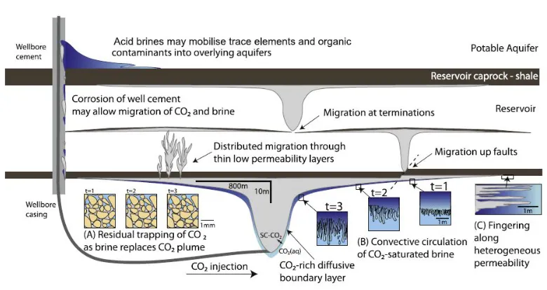
Geological storage relies on the injection of CO2 into porous rock formations (Holloway, 2001; Friedmann, 2007; Benson and Cole, 2008). It involves separating CO2 at power stations or other industries plants, compressing it, transporting to the storage site and injecting it into permeable strata at depths. Sedimentary basins are considered suitable as CO2 storage reservoirs (Oelkers and Cole, 2008). Reservoir formations are deep aquifers covered by very low permeability formations that act as a caprock. An impermeable caprock is essential because CO2 density is generally less than that of water at depth temperature and pressure conditions, so buoyancy tends to drive CO2 upwards, back to the surface. Several industrial-scale geologic CO2 storage programs are already underway, including the Norwegian Sleipner project in the North Sea (Korbøl and Kaddour, 1995) and the Weyburn project in Canada (Emberley et al., 2005); at these sites, a million tons or more of CO2 is injected into the subsurface each year. Moreover, other current worldwide CCS projects are currently running (In Salah (Algeria), K12B (Netherlands), Snøhvit (Norway) among others). Some of these storage sites also consist of exploited gas or fuel reservoirs, and CO2 injection is used to enhance oil recovery.
Chapter I
[image:41.595.100.490.99.306.2]|6
Figure 1.3Diagrammatic illustration of geological carbon storage. CO2 from concentrated sources is separated from
other gasses compressed and injected into porous geological strata at depths >800 m where it is in a dense or supercritical phase. The CO2 is lighter than formation brines, rises and is trapped by impermeable strata. The risks
are that the light CO2 will exploit faults or other permeable pathways to escape upwards and acid CO2-charged brines might corrode the caprocks or fault zones (Kampman et al., 2014).
The criteria for suitability are, first, that there is sufficient pore volume to store a significant portion of CO2 emissions, second, that there is a structural trap with enough integrity to contain the buoyant CO2 for hundreds to thousands of years and third, that permeability is high enough to inject at high flow rate.
1.3 CO2 leakage through caprock and wells
Introduction
|7
1.3.1 Caprock
Investigating the interaction between the caprock and CO2-rich brine through potential pathways is of paramount importance to evaluate the long-term caprock sealing capacity (Kaszuba et al., 2005; Noiriel et al., 2007; Andreani et al., 2008; Busch et al., 2008; Hangx et al., 2010; Ellis et al., 2011; Berrezueta et al., 2013; Smith et al. , 2013). Acidified CO2-rich brines may react with caprock minerals that are susceptible to dissolve, releasing ions into the solution that could lead to mineral precipitation (Knauss et al., 1993; Brady and Carroll, 1994, Pokrovsky et al., 2009; Hellmann et al., 2010; Smith and Carroll, 2014). Mineral dissolution rates relevant to the reactions taking place under these conditions were previously obtained (Chou and Wollast, 1985; Jeschke et al., 2001; Domènech et al., 2002; Köhler et al., 2003; Palandri and Kharaka, 2004; Lowson et al., 2007; Bandstra et al., 2008; Xu et al., 2012; Smith et al., 2013). Mineralogical changes affect porosity, pore structure and hydrodynamic and mechanical properties of caprocks (Park et al., 2011; Vilarrasa et al., 2013).
In the last decade, caprock reactivity in CO2-rich solutions has been studied using batch and flow-through experiments (Kaszuba et al., 2005; Kohler et al., 2009; Alemu et al., 2011; Credoz et al., 2011; Liu et al., 2012; Garrido et al., 2013). The authors reported significant mineral alterations and changes in pore volume owing to dissolution and precipitation of carbonate and clay minerals, illitization of smectite and formation of swelling clays. Flow-through laboratory-scale experiments under atmospheric and supercritical CO2 conditions have been conducted to better understand how the caprock reactivity may affect the hydraulic and mechanical properties of the rocks. In these experiments, core and fractured core samples made up of marl, shale, limestone or evaporite rocks were used (Noiriel et al., 2007; Andreani et al., 2008; Angeli et al., 2009; Berrezueta et al., 2013; Ellis et al., 2011; Deng et al., 2013; Smith et al., 2013). Other mineral alterations including reorganization of clay minerals in a fracture and an altered layer on the fracture surface led to variations in fracture permeability (Noiriel et al., 2007; Andreani et al., 2008).