(gamma)-ray emission from regions of star formation: Theory and observations with the MAGIC Telescope

Texto completo

(1)Universitat Autònoma de Barcelona. γ-ray emission from regions of star formation: Theory and observations with the MAGIC Telescope Ph.D. Dissertation. Eva Domingo Santamarı́a. March 2006. supervised by Juan Cortina Blanco & Diego F. Torres. Universitat Autònoma de Barcelona Departament de Fı́sica Institut de Fı́sica d’Altes Energies (IFAE) Edifici C-n, Campus UAB, E-08193 Bellaterra (Barcelona).

(2) 2.

(3) A todos ellos, por la fuerza que me han dado.. i.

(4) ii.

(5) Agradecimientos Quisiera comenzar agradeciendo a todos aquellos que en su dı́a me dieron la oportunidad de pasar 6 años de mi vida en el mundo de la investigación, empezando por Enrique Fernández por acogerme en el IFAE, y terminando por Manel Martı́nez, quien me abrió una puerta al fascinante mundo de MAGIC y la astrofı́sica de altas energı́as. Una vez ahı́ las vivencias, las personas, los momentos, las dificultades, los nervios, las ilusiones, han sido muchas y muy variadas. Pero sin duda, si pienso en esta tesis, son dos las personas a quienes más debo mi agradecimiento: mis directores, Juan Cortina y Diego Torres. Es mucho lo que he aprendido con y gracias a ellos, Juan, enseñándome los entresijos del telescopio y del análisis de los datos, y Diego ayudándome a atreverme con la teorı́a y los modelos y a disfrutar con la fı́sica de los poderosos objetos que MAGIC observa. Ambos cercanos, ambos implicados, mucho más no se puede pedir. Cada cual con su opinión (no siempre la misma) pero siempre manteniendo esa combinación de profesionalidad, respeto, cercanı́a y confianza, que sé tan difı́cil de lograr (y más entre 3 personas), y que sin duda ha sido la base de que haya sido capaz de hacer y poner por escrito todo este trabajo. Y sı́, es cierto, me siento afortunada, para mi han sido la combinación perfecta. Gracias a los dos por vuestra confianza, vuestra paciencia y vuestro esfuerzo, que sé que no ha sido poco, espero trasmitiros lo mucho que lo aprecio. La verdad es que trabajar en la colaboración MAGIC ha sido un gran placer, ya no sólo porque me ha permitido empezar a imaginar un poco mejor todo esa enormidad que nos rodea, sino que también (y sobretodo) por el genial ambiente humano que tantos han logrado crear siempre. Están los magicians del IFAE. Primero con quienes empecé tirando cables ahi arriba en La Palma y de quien he acabado aprendiendo tanto porque siempre han estado ahı́, para echar una mano: Oscar, que se fue a Paris pero sigue estando siempre cerca; Pepe, con quien he tenido el placer de trabajar codo a codo y desesperarnos y emocionarnos juntos; Javi, que siempre tuvo un minuto y una sonrisa amable; y Markus, siempre dispuesto a ayudar. Y no me quiero olvidar de Xavi, y nuestras bombillas disipadoras de calor, ni de Jose, que siempre tuvo una solución para todo y que me enseñó de cables y de charlas tranquis. Luego están los que llegaron más tarde y que espero que no nos maldigan mucho por lo que les hayamos dejado: Ester y Núria, mis compañeras de despacho en alguna de mis mudanzas, gracias por las ayudas en todos los sentidos, Roger y nuestro cooling y sus fabulosos scripts, Alex y su genial ironı́a, Manel y Diego, y Javi (gracias por las discusiones) y Emma (gracias por la luna). Pero el mundo magician sigue fuera de las paredes del IFAE. En especial quiero agradecer las charlas, los emails, las discusiones, los ratos, las ayudas, los viajes a Wolfgang, Abelardo, Pratik, Florian, Ciro, Nadia, Nepomuk, Antonio, Arnau, Dorota, Fabrizio, Raquel, Andreu, Daniela, Villi, Toni, el otro Daniel... y a tantos otros... Pero el dı́a a dı́a no ha sido sólo MAGIC, puesto que el IFAE es grande y muchos han sido los que han alimentado las ganas de estar allı́. Primero mi Laieta, que estuvo el iii.

(6) primer año que llegué, se fue al CERN, le dio tiempo a volver, y sigue como siempre, aún más cercana. Luego Ana y nuestras escasas pero valiosas charlas. Y Carlos y su dulzura. Sigrid y sus sonrisas. Y Ester, que nos mantiene activos. Y Jose, Gabriel, Natalia, Magali, Alex y Mireia, y Olga y Xavi desde los USA. Antes de salir del mundo de la investigación, que tantas horas me ha retenido, quiero acordarme de Magda, mi gran amiga mexicana, con quien tan buenos momentos he pasado y con quien charlar, de fı́sica y no fı́sica, siempre ha sido un placer y un aprendizaje. Y, bueno, aún quedan por ahı́ mi pandilla de fı́sicos (y no fı́sicos) que al final han acabado rondado casi todos siempre por la uni. Felisa, que tanto me conoce y siempre tanto me da, a menudo sin darse cuenta. Marieta, que no podrı́a no cuidarnos a todos. Juanma, siempre atento y dispuesto a dar un abrazo a la hora que sea. Y Ro, que no nos falten sus sueños y sus locuras. Y el bueno de Ángel, y la silenciosa Marcel·la. Gracias por todos los buenos ratos y vuestro respaldo. Y prepararos, que ya vuelvo a por mi vida social. Luego están y han estado, a quienes veo menos, por pura distancia (calculada desde mi asiento en el despacho del fondo del pasillo del IFAE). Jose Luis y lo mucho compartido y conservado, mi Evita y su cariño, Mateo y sus rizos amables, Ramon y sus inquietudes, Paquita y su manera de cuidarme, Zaida y sus emails dando ánimos cuando más falta hacen, Sergio y el gran aprecio que hay, Montse y su ternura, Josep y su locura, Yanina y nuestra amistad y ese viaje, Susana y los buenos reencuentros, y Raquel y Diego que siempre me esperan en mi Salou, con el mar. No me quiero dejar esta vez a mi familia, tı́os y tı́as, primos y primas, más o menos cercanos, que no han parado de interesarse por lo que hacı́a, de asaltarme alguna vez con preguntas que jamás me habı́a planteado, y que ahora ’amenazan’ con venir, desde donde haga falta, a apoyarme en la recta final. Y para acabar, los mı́os. Mi hermano, aunque ausente siempre presente. Mi hermanita, ya ALBA con todas las letras bien puestas, por su cariño, su apoyo, nuestras charlas y su esfuerzo por seguir fortaleciendo dı́a a dı́a nuestra relación que tanto bien me hace. Y mis padres, que siempre están ahı́, dándome fuerzas y apoyo, aunque yo a veces no me deje. Gracias por cuidarme, por quererme y demostrármelo, y por haber confiado siempre en mı́. A todos, gracias por lo aprendido y compartido, y por aguantar de cerca mis nervios e inestabilidades y, de lejos, mis largas ausencias.. iv.

(7) Contents List of Figures. ix. List of Tables. xxi. 1 Introduction: Astrophysics with γ-rays 1.1 The experimental status at GeV energies . . . . . . . . . . . . . . . . . . . 1.2 The experimental status at TeV energies . . . . . . . . . . . . . . . . . . . 1.3 This thesis . . . . . . . . . . . . . . . . . . . . . . . . . . . . . . . . . . . .. 1 2 3 6. I. 9. Theory and phenomenology of regions of star formation. 2 Extragalactic sites of star formation: Phenomenology 2.1 Diffuse γ-ray emission from galaxies . . . . . . . . . . . . . . . . . . . . 2.1.1 Diffuse γ-ray emission from the Galaxy . . . . . . . . . . . . . . 2.1.2 Detection (and non-detection) of other local group galaxies . . . 2.2 Galaxies with higher star formation rate . . . . . . . . . . . . . . . . . . 2.2.1 Plausibility estimation . . . . . . . . . . . . . . . . . . . . . . . . 2.2.2 The HCN and the Pico Dos Dias surveys: looking for candidates 2.2.3 Requirements for detection . . . . . . . . . . . . . . . . . . . . . 2.3 Concluding remarks . . . . . . . . . . . . . . . . . . . . . . . . . . . . .. . . . . . . . .. 11 11 12 13 16 18 20 22 24. 3 Extragalactic sites of star formation: Modeling 3.1 Emission model of the nearest starburst galaxy . . . . . . 3.1.1 CANGAROO GeV-TeV observations of NGC 253 3.1.2 Phenomenology of the central region of NGC 253 . 3.1.3 Diffuse modeling . . . . . . . . . . . . . . . . . . . 3.1.4 Results . . . . . . . . . . . . . . . . . . . . . . . . 3.1.5 HESS observations of NGC 253 . . . . . . . . . . . 3.1.6 Summary of NGC 253 modeling . . . . . . . . . . 3.2 Comments on an emission model of the nearest ULIRG . 3.2.1 Some words on phenomenology of Arp 220 . . . . 3.2.2 High energy γ-ray fluxes and observability . . . . . 3.3 Concluding remarks . . . . . . . . . . . . . . . . . . . . .. . . . . . . . . . . .. 25 25 25 26 29 32 40 41 43 44 45 46. v. . . . . . . . . . . .. . . . . . . . . . . .. . . . . . . . . . . .. . . . . . . . . . . .. . . . . . . . . . . .. . . . . . . . . . . .. . . . . . . . . . . .. . . . . . . . . . . ..

(8) 4 Galactic sites of star formation: OB associations 4.1 Introduction . . . . . . . . . . . . . . . . . . . . . . . . . . 4.2 The gas within a collective wind . . . . . . . . . . . . . . 4.3 Mass loss rates and terminal velocities of individual stars 4.4 Modulation and counterparts . . . . . . . . . . . . . . . . 4.5 Secondaries from a cosmic ray spectrum with a low energy 4.5.1 The normalization of the cosmic ray spectrum . . 4.5.2 Emissivities . . . . . . . . . . . . . . . . . . . . . . 4.5.3 Electron energy losses and distribution . . . . . . . 4.5.4 Total γ-ray flux from a modulated environment . . 4.6 Opacity to γ-ray escape . . . . . . . . . . . . . . . . . . . 4.7 Candidates: Cygnus OB 2 and Westerlund 1 . . . . . . . 4.8 Concluding Remarks . . . . . . . . . . . . . . . . . . . . .. II. . . . . . . . . . . . . . . . . cutoff . . . . . . . . . . . . . . . . . . . . . . . . . . . .. . . . . . . . . . . . .. . . . . . . . . . . . .. . . . . . . . . . . . .. . . . . . . . . . . . .. . . . . . . . . . . . .. The MAGIC Telescope and data analysis method. 67. 5 The Čerenkov technique and the MAGIC Telescope 5.1 Extended Air Showers . . . . . . . . . . . . . . . . . . . . . . . . . 5.1.1 Electromagnetic EAS . . . . . . . . . . . . . . . . . . . . . 5.1.2 Hadronic EAS . . . . . . . . . . . . . . . . . . . . . . . . . 5.2 The Imaging Atmospheric Čerenkov Technique . . . . . . . . . . . 5.2.1 Čerenkov radiation in an EAS . . . . . . . . . . . . . . . . . 5.2.2 Imaging Air Čerenkov Telescopes: detection technique . . . 5.3 The MAGIC Telescope . . . . . . . . . . . . . . . . . . . . . . . . . 5.3.1 The telescope frame, reflector mirror dish and drive system 5.3.2 The camera of the MAGIC Telescope . . . . . . . . . . . . 5.3.3 The trigger and the data acquisition systems . . . . . . . . 5.3.4 The calibration system . . . . . . . . . . . . . . . . . . . . . 5.3.5 The control system . . . . . . . . . . . . . . . . . . . . . . . 6 Data analysis method 6.1 Sources of background . . . . . . . . . . . . . . . . . . . . 6.2 Monte Carlo simulation . . . . . . . . . . . . . . . . . . . 6.3 First selection of the data sample . . . . . . . . . . . . . . 6.3.1 Types of data runs . . . . . . . . . . . . . . . . . . 6.3.2 Run selection . . . . . . . . . . . . . . . . . . . . . 6.4 Calibration, cleaning and image parameterization . . . . . 6.4.1 Signal extraction . . . . . . . . . . . . . . . . . . . 6.4.2 Pedestal evaluation and subtraction . . . . . . . . 6.4.3 Calibration of the signal . . . . . . . . . . . . . . . 6.4.4 Identification of bad pixels . . . . . . . . . . . . . 6.4.5 Image cleaning . . . . . . . . . . . . . . . . . . . . 6.4.6 Parameterization of the EAS shower images: Hillas 6.5 Second selection . . . . . . . . . . . . . . . . . . . . . . . 6.5.1 Run quality checks . . . . . . . . . . . . . . . . . . 6.5.2 Event quality cuts . . . . . . . . . . . . . . . . . . 6.5.3 γ/hadron separation . . . . . . . . . . . . . . . . . vi. 48 48 49 52 55 57 57 58 59 61 62 63 65. . . . . . . . . . . . .. . . . . . . . . . . . .. . . . . . . . . . . . .. 69 69 70 71 72 72 77 80 81 83 88 90 92. . . . . . . . . . . . . . . . . . . . . . . . . . . . . . . . . . . . . . . . . . . . . . . . . . . . . . . . . . . . . . . . . . . . . . . . . . . . . . parameters . . . . . . . . . . . . . . . . . . . . . . . . . . . .. . . . . . . . . . . . . . . . .. . . . . . . . . . . . . . . . .. 93 93 94 96 96 97 98 98 100 100 101 102 102 105 105 107 109. . . . . . . . . . . . ..

(9) 6.6. 6.7. III. 6.5.4 Optimization of hadronness and alpha cut Reconstruction of primary parameters . . . . . . 6.6.1 Energy reconstruction . . . . . . . . . . . 6.6.2 Source position reconstruction . . . . . . Evaluation of the signal . . . . . . . . . . . . . . 6.7.1 Significance calculation . . . . . . . . . . 6.7.2 Flux sensitivity . . . . . . . . . . . . . . . 6.7.3 Upper limit calculation . . . . . . . . . .. . . . . . . . .. . . . . . . . .. . . . . . . . .. . . . . . . . .. . . . . . . . .. . . . . . . . .. . . . . . . . .. . . . . . . . .. . . . . . . . .. . . . . . . . .. . . . . . . . .. . . . . . . . .. . . . . . . . .. . . . . . . . .. First MAGIC observations of regions of star formation. 7 Evaluating the MAGIC sensitivity with Crab 7.1 Characteristics of the source and previous observations 7.2 Analysis procedure . . . . . . . . . . . . . . . . . . . . 7.3 Data sample . . . . . . . . . . . . . . . . . . . . . . . . 7.4 Data quality checks . . . . . . . . . . . . . . . . . . . . 7.4.1 Event rate . . . . . . . . . . . . . . . . . . . . . 7.4.2 Hillas parameters distributions . . . . . . . . . 7.5 Optimal cuts and flux sensitivities . . . . . . . . . . . 7.6 Estimation of the telescope angular resolution . . . . . 8 MAGIC observations of Arp 220 8.1 Characteristics of the source and previous observations 8.2 Data sample . . . . . . . . . . . . . . . . . . . . . . . . 8.3 Data quality checks . . . . . . . . . . . . . . . . . . . . 8.3.1 Event rate . . . . . . . . . . . . . . . . . . . . . 8.3.2 Hillas parameter distributions . . . . . . . . . . 8.3.3 Evaluation of the mispointing . . . . . . . . . . 8.4 ALPHA plots and Upper limits from Crab sensitivity . 9 MAGIC observations of TeV J2032+4130 9.1 Characteristics of the source and previous observations 9.2 Data sample . . . . . . . . . . . . . . . . . . . . . . . . 9.3 Data quality checks . . . . . . . . . . . . . . . . . . . . 9.3.1 Event rate . . . . . . . . . . . . . . . . . . . . . 9.3.2 Hillas parameter distributions . . . . . . . . . . 9.4 ALPHA plots and flux upper limits . . . . . . . . . . . 9.5 Conclusions . . . . . . . . . . . . . . . . . . . . . . . . 10 Concluding remarks. . . . . . . . .. . . . . . . .. . . . . . . .. . . . . . . . .. . . . . . . .. . . . . . . .. . . . . . . . .. . . . . . . .. . . . . . . .. . . . . . . . .. . . . . . . .. . . . . . . .. . . . . . . . .. . . . . . . .. . . . . . . .. . . . . . . . .. . . . . . . .. . . . . . . .. 112 116 116 120 123 123 124 125. 127 . . . . . . . .. . . . . . . .. . . . . . . .. . . . . . . . .. . . . . . . .. . . . . . . .. . . . . . . . .. . . . . . . .. . . . . . . .. . . . . . . . .. . . . . . . .. . . . . . . .. . . . . . . . .. 129 129 130 132 133 136 136 138 144. . . . . . . .. 147 147 147 149 149 149 149 153. . . . . . . .. 158 158 161 162 162 165 166 171 173. A A numerical approach for multiwavelength modeling 175 A.1 Q-diffuse flow and concept . . . . . . . . . . . . . . . . . . . . . . . . . . 175 B γ-ray emission from neutral pion decay 178 B.1 Neutral pion and γ-ray emissivities . . . . . . . . . . . . . . . . . . . . . . 178 B.1.1 Limits of the integrals . . . . . . . . . . . . . . . . . . . . . . . . . 181 vii.

(10) B.2 Parameterizations of cross sections for neutral pion production in proton-proton collisions . . . . . . . . . . . . . . . . . . . . . . . . . . . . . . . . . . . . . 183 B.2.1 The δ-function approximation and a total cross section parameterizations . . . . . . . . . . . . . . . . . . . . . . . . . . . 184 B.2.2 Differential cross section parameterizations . . . . . . . . . . . . . 186 C Physics included in the numerical modeling C.1 Energy loss processes . . . . . . . . . . . . . . . . . . . . . C.1.1 Proton losses . . . . . . . . . . . . . . . . . . . . . C.1.2 Electron losses . . . . . . . . . . . . . . . . . . . . C.2 Secondary production processes . . . . . . . . . . . . . . . C.2.1 Electrons from knock-on (or Coulomb) interactions C.2.2 Electrons and positrons from charged pion decay . C.3 Radiative processes . . . . . . . . . . . . . . . . . . . . . . C.3.1 Radio and Infrared emission . . . . . . . . . . . . . C.3.2 High energy emission . . . . . . . . . . . . . . . . . C.4 Opacities to γ-ray escape . . . . . . . . . . . . . . . . . . C.5 Radiation transport equation and fluxes from emissivities . . . . . . . . . . . . . . . . . . . . D Camera subsystems controlled by PLCs D.1 PLCs and Modbus control . . . . . . . . D.2 Camera subsystems . . . . . . . . . . . . D.2.1 The camera lids . . . . . . . . . D.2.2 The camera cooling system . . .. . . . . . . . . . .. . . . . . . . . . .. . . . . . . . . . .. . . . . . . . . . .. . . . . . . . . . .. . . . . . . . . . .. . . . . . . . . . .. . . . . . . . . . .. . . . . . . . . . .. 190 190 190 192 196 196 197 201 201 204 205. . . . . . . . . . 206 . . . .. 209 209 210 210 211. E Focusing quality of the telescope E.1 Comparison of MC simulated and real γ events . . . . . . . . . . . . . . . E.2 Comparison with muon studies . . . . . . . . . . . . . . . . . . . . . . . . E.3 Conclusion: the selected MC sample . . . . . . . . . . . . . . . . . . . . .. 216 216 217 221. Bibliography. 223. viii. . . . .. . . . .. . . . .. . . . .. . . . .. . . . .. . . . .. . . . .. . . . .. . . . .. . . . .. . . . .. . . . .. . . . .. . . . .. . . . .. . . . .. . . . ..

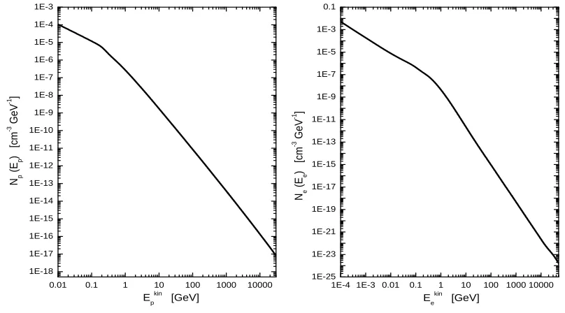
(11) List of Figures 1.1 1.2 1.3 1.4 1.5. 2.1. 2.2 2.3. 2.4. 2.5. 2.6. 3.1. 3.2. The EGRET point-like sources γ-ray sky. About 170 significant signals are still unidentified sources. . . . . . . . . . . . . . . . . . . . . . . . . . . . . Simulated predictions of the one-year all-sky survey of the LAT experiment. Current ground-based experiments operating in the high energy γ-ray domain. Significance map of the H.E.S.S. 2004 Galactic plane scan. 8 high significant sources have been detected. From Aharonian et al. (2005e). . . . . . . . . The Very High Energy γ-ray sky in 2005. Not shown are 8 more sources discovered by HESS in a survey of the galactic plane. Red symbols indicate the most recent detections, brought during 2004 and 2005 by the last generation of IACTs: HESS and MAGIC. From Ong (2005). . . . . . . . . Intensity of γ-rays (> 100 MeV) observed by EGRET. The broad, intense band near the equator is interstellar diffuse emission from the Milky Way. The intensity scale ranges from 1×10−5 cm−2 s−1 sr−1 to 5×10−4 cm−2 s−1 sr−1 in ten logarithmic steps. The data is slightly smoothed by convolution with a gaussian of FWHM 1.5◦ . . . . . . . . . . . . . . . . . . . . . . . . . The Milky Way in molecular material and γ-rays. An obvious correlation favors the idea of a diffuse generation of high energy radiation. . . . . . . Spectrum of the inner Milky Way (|l| < 60◦ , |b| < 10◦ ) with calculated components from bremsstrahlung (EB), inverse Compton (IC), neutral pion decay (NN), and extragalactic isotropic emission (ID). . . . . . . . . . . . LMC as seen by EGRET (γ-rays) and IRAS (infrared). White circle indicates the position of 30 Doradus, a large molecular cloud and intense star formation region. By courtesy of Seth Digel. . . . . . . . . . . . . . Distribution of luminosity distances (insets) and minimum average CR enhancements needed for galaxies in the HCN (left) and Pico Dos Dias (right) surveys to appear as γ-ray sources for GLAST and the new ground based Čerenkov telescopes. . . . . . . . . . . . . . . . . . . . . . . . . . . Plausible values of enhancements for the HCN galaxies obtained as the ratio between the SFR of each galaxy and that of the Milky Way versus the needed one for them to be detectable by GLAST. LIRGs (less luminous galaxies) are shown as white points (black) points. See text for discussion. An optical image of NGC 253. The high value of inclination, and the grand-design type of this galaxy makes of it one of the most spectacular objects in the sky. . . . . . . . . . . . . . . . . . . . . . . . . . . . . . . . Steady proton (left panel) and electron (right panel) distributions in the innermost region of NGC 253. . . . . . . . . . . . . . . . . . . . . . . . . . ix. 2 3 4 5. 6. 12 13. 14. 15. 21. 24. 27 34.

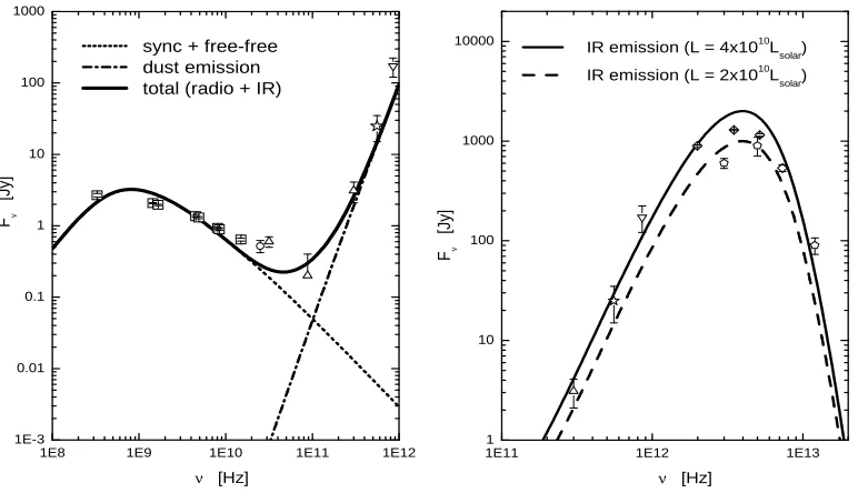
(12) 3.3. 3.4. 3.5. 3.6. 3.7. 3.8. 3.9. Left: Ratio of the steady proton population in the surrounding disk to that in the innermost starburst region. Right: Ratio between the steady proton distribution in the IS, when the gas density is artificially enhanced and diminished by a factor of 2. . . . . . . . . . . . . . . . . . . . . . . . .. 35. Steady population of primary-only and secondary-only electrons. Only the region of the secondary dominance of the distribution is shown. . . . . .. 36. Left: IR flux from NGC 253 assuming a dilute blackbody with temperature Tdust = 50 K and different total luminosities. Right: Multifrequency spectrum of NGC 253 from radio to IR, with the result of this modeling. The experimental data points correspond to: pentagons, Melo et al. (2002); diamonds, Telesco et al. (1980); down-facing triangles, Rieke et al. (1973); stars, Hildebrand et al. (1977); up-facing triangles, Elias et al. (1978); circles, Ott et al. (2005); squares, Carilli (1996). . . . . . . . . . . . . . .. 37. Left: Differential γ-ray fluxes from the central region of NGC 253. Total contribution of the surrounding disk is separately shown, as are the EGRET upper limits. In the case of the IS, the contributions of bremsstrahlung, inverse Compton, and neutral pion decay to the γ-ray flux are also shown. Right: Integral γ-ray fluxes. The EGRET upper limit (for energies above 100 MeV), the CANGAROO integral flux as estimated from their fit, and the HESS sensitivity (5σ detection in 50 hours) are given. Absorption effects are already taken into account. Also shown is the recently released HESS upper limit curve on NGC 253. . . . . . . . . . . . . . . . . . . . .. 38. Left: Opacities to γ-ray scape as a function of energy. The highest energy is dominated by γγ processes, whereas γZ dominates the opacity at low energies. Significant τmax are only encountered above 1 TeV. Right: Detail of the modification of the γ-ray spectrum introduced by the opacity to γ-ray escape. . . . . . . . . . . . . . . . . . . . . . . . . . . . . . . . . . .. 39. Proton distribution when different convective and the pp timescales are taken into account as compared with a (arbitrary) solution when τ (E) = τD , i.e., diffusion only. Clearly, convection plus pp timescales dominates the spectrum. . . . . . . . . . . . . . . . . . . . . . . . . . . . . . . . . .. 40. Left: Energy density contained in the steady population of protons above the energy given by the x-axis. Right: Cosmic ray enhancement factor obtained from the steady spectrum distribution in the innermost starburst nucleus of NGC 253. . . . . . . . . . . . . . . . . . . . . . . . . . . . . . .. 41. 3.10 Top left: Angular distribution of γ-like images relative to the centre of NGC 253 (On) and relative to the background control region (Off) for HESS Analysis method 1. Events are plotted versus the squared angular distance to give equal solid angle in each bin. Background curves (histograms) are determined relative to points 1 degree away from the source position. Top right: idem but using HESS Analysis method 2 (for description of these two methods see Aharonian et al. (2005c). Courtesy of the HESS collaboration. 42 x.

(13) 3.11 Left: γ-ray point source significance map (grey-scale) derived from two telescope HESS data taken in August and September 2004, using Analysis 1. The white contours show the optical emission from the galaxy (in a linear scale) using data from the STScI Digitized Sky Survey. Black contours are confidence levels (at 40%, 65% and 80%) for TeV γ-ray emission reported by CANGAROO collaboration. The dashed white line shows the angular cut used to derive extended source flux limits. Right: Significance map derived from the same dataset using Analysis 2. In contrast to the left panel the statistical significance in each bin is independent. The bin size is matched to the angular resolution of the instrument for these data. Courtesy of the HESS collaboration. . . . . . . . . . . . . . . . . . . . . . . . . . . . . . .. 42. 3.12 Integral γ-ray fluxes produced in this model zoomed in the region above 100 GeV. The CANGAROO integral flux as estimated from their fit, and the HESS sensitivity (5σ detection in 50 hours) are given, together with HESS upper limits. Absorption effects are already taken into account. . .. 43. 3.13 A near-infrared image of the peculiar galaxy Arp 220 from the Hubble Space Telescope. More luminous than 100 Milky Ways and radiating most of its energy in the infrared, Arp 220 is a ULIRG. It is likely the result of a collision of 2 spiral galaxies. . . . . . . . . . . . . . . . . . . . . . . . . .. 44. 3.14 Geometry and different components in the model of Arp 220. Two central spherical nuclei are extreme regions of star formation, and co-rotate with the molecular disk. . . . . . . . . . . . . . . . . . . . . . . . . . . . . . .. 46. 3.15 Total integral flux predictions for Arp 220. The dashed line shows the results obtained with the Q-diffuse numerical package using Blattnig et al. (2000) parameterization of the pp cross section; the solid line shows the fluxes obtained with the same model but using other cross sections (Aharonian & Atoyan, or Kamae et al.). The HESS and MAGIC telescopes sensitivities, 50 hours of observation time for a 5σ detection, for low zenith angles (although note that this is shown here just for quick comparison, since HESS can only observed Arp 220 above ∼ 50◦ ), are also shown to remark the differences in predictions for observability that the use of one or other cross section can induce. Absorption effects are already taken into account in both cases. . . . . . . . . . . . . . . . . . . . . . . . . . . . . .. 47. 4.1. 4.2. Schematic diagram showing the wind-wind interaction that takes place in a dense stellar cluster or sub-cluster. The stars are assumed to be uniformly distributed within the outer radius of the cluster. The material ejected from the Rc stars goes through stellar wind shocks (drawn as circles) and then participates in an outward flow [with mean velocity V (R) and density n(R)] which eventually leaves the cluster and interacts with the surrounding interstellar matter. After Canto et al. (2000). . . . . . . . . .. 49. Examples of configurations of collective stellar winds. Main parameters are as in Table 1. . . . . . . . . . . . . . . . . . . . . . . . . . . . . . . . . . .. 53. xi.

(14) 4.3. 4.4. 4.5. 4.6. 5.1. Contribution of cosmic rays of different energies to the hadronic γ-ray emissivity. The medium density is normalized to 1 cm−3 and the cosmic ray spectrum is proportional to E −2.3 (black) and E −2.0 (grey), with an enhancement of a thousand when compared with the Earth-like one above 1 GeV. The normalization of each spectrum (of each slope) is chosen to respect the value of enhancement. In the case of the harder spectrum of α = 2.0, only the results for the whole cosmic ray spectrum are shown, but a similar decrease in emissivity to that of α = 2.3 can be observed if lower energy cutoffs are imposed. . . . . . . . . . . . . . . . . . . . . . . . . . .. 58. The effect of a modulated cosmic ray spectrum (the same as in Figure 4.3 with α = 2.3 and 2.0) over the electron knock-on emissivity (left) and the positron emissivity (middle) of a medium with density n = 1 cm−3 . Right: Different losses for assumed parameters: Curves 1 correspond to ionization losses for n = 100 and 20 cm−3 . Curves 2 correspond to synchrotron losses for B = 50 and 200 µG (see text). Curves 3 correspond to inverse Compton losses for a photon energy density of 20 and 100 eV cm−3 . Curves 4 correspond to Bremsstrahlung losses for n = 100 and 20 cm−3 . Curve 5 corresponds to adiabatic losses having a ratio V (km s−1 )/R(pc)=300 (e.g., a wind velocity of 1500 km s−1 and a size relevant for the escape of the electrons of 5 pc). . . . . . . . . . . . . . . . . . . . . . . . . . . . . . . . .. 59. Secondary electron distribution obtained by numerically solving the loss equation. The primary cosmic ray spectrum is the same as in Figure 4.3 with α = 2.3, and results are shown for different low energy cutoffs. The average density is assumed as n = 20 cm−3 , the magnetic field is assumed as 50 µG, and the size relevant to escape the modulating region is 5 pc. The inset shows the total energy loss rate b(E). . . . . . . . . . . . . . . .. 60. Differential (left panel) and integral (right panel) fluxes of γ-rays emitted in a non-modulated and a modulated environment. The bump at very low energies in the left panel is produced because leptonic emission coming only from secondary electrons is shown. Above ∼ 70 MeV the emission is dominated by neutral pion decay. Also shown are the EGRET, GLAST, MAGIC and HESS sensitivities. Note that a source can be detectable by IACTs and not by GLAST, or viceversa, depending on the slope of the cosmic ray spectrum and degree of modulation. Right: Opacities to γγ pair production in the soft photon field of an O4V-star at 10, 100 and 1000 R⋆ , and in the collective photon field of an association with 30 stars distributed uniformly over a sphere of 0.5 pc. The closest star to the creation point is assumed to be at 0.16 pc, and the rest are placed following the average stellar density as follows: 1 additional star within 0.1, 2 within 0.25, 4 within 0.32, 8 within 0.40 and 14 within 0.5 pc. . . . . . . . . . . . . . . .. 61. Sketch of the structure and the interactions present in an EAS, induced by a cosmic γ-ray (left) and by a charged cosmic nucleus (right). . . . . . . .. 70. xii.

(15) 5.2. Simulation of an electromagnetic (left panels) and hadronic (right panels) Extended Air Showers. The top panels show the development of the shower in the atmosphere and the bottom ones the angular distribution of the Čerenkov photons at ground levels. Evident morphological differences can be seen which are crucial for imaging-based background substraction methods. . . . . . . . . . . . . . . . . . . . . . . . . . . . . . . . . . . . .. 73. Polarization of the medium induced by a charged particle with low velocity (a) and with high velocity (b). Huygens construction of Čerenkov waves that only finds coherence for the Čerenkov angle θč with respect to the charged particle trajectory (c). . . . . . . . . . . . . . . . . . . . . . . . .. 74. Scheme of the Čerenkov light ring produced by an ultra-relativistic charged particle at the observation level. The first two beams on panel (a) hit the ground at roughly the same radial distance even if they are produced at different heights. Panel (b) shows the simulation of the Čerenkov light pool produced by γ-ray and proton showers. The γ-induced Čerenkov light profile is practically constant until a radius of a hundred meters, where the hump occurs, and then decay rapidly for higher radius. Taken from Paneque (2004). . . . . . . . . . . . . . . . . . . . . . . . . . . . . . . . . .. 75. Differential Čerenkov photon spectrum in arbitrary units in the ultraviolet and visible wavelength ranges, emitted at 10 km above sea level (dotted line) and detected at 2 km (solid line) after suffering absorption in the Ozone layer and Rayleigh and Mie scattering. Graphic taken from Moralejo (2000). . . . . . . . . . . . . . . . . . . . . . . . . . . . . . . . . . . . . . .. 77. Sketch of the principle of the Čerenkov technique, through the formation of the image of an EAS in an IACT pixelized camera. The numbers in the figure correspond to a typical 1 TeV γ-ray induced shower. . . . . . . . .. 78. Čerenkov photon density at 2km height above sea level for different type of incident primary particles and as a function of their energy. Figure taken from Ong (1998). . . . . . . . . . . . . . . . . . . . . . . . . . . . . . . . .. 79. The MAGIC Telescope at ”El Roque de los Muchachos” site in the canary island of La Palma. . . . . . . . . . . . . . . . . . . . . . . . . . . . . . . .. 82. Scheme of the MAGIC camera layout. The inner region (in blue) is equipped with 0.1◦ ø FOV pixels to get a better sampling of the low energy showers. The outer region (in red) is segmented in 0.2◦ ø FOV pixels. The whole camera FOV is 3.5-3.8◦ in diameter. . . . . . . . . . . . . . . . . . . . . .. 84. 5.10 Front view of the MAGIC Telescope camera. The plexiglas window protects the camera interior where the light concentrators collect the incident light onto the camera photosensors. . . . . . . . . . . . . . . . . . . . . . . . . .. 85. 5.11 Scheme of the signal flow and the data readout in the MAGIC Telescope.. 87. 5.12 The trigger macrocells in the inner region of the MAGIC camera. . . . . .. 89. 5.3. 5.4. 5.5. 5.6. 5.7. 5.8 5.9. 6.1. The V extinction coefficient from 1984 to 2005 as measured by the Carlsberg Meridian Telescope. The effect of the eruption of Mount Pinatubo in June 1991 is clearly visible. The number of high extinction values that occur every summer is normally caused by Saharan dust. . . . . . . . . . . . . . xiii. 99.

(16) 6.2. Identification of bad pixels from the analysis of a calibration run. On the left, the excluded pixels are colored in the camera layout drawing and the reason for their tagging as unsuitable is given in the list above. On the right, pixels showing a behavior deviated from the expected mean are tagged as unreliable but still keep by default for further analysis. . . . . . . . . . . . 101. 6.3. Scheme of the parameterization of shower images with an ellipse as proposed by Hillas. . . . . . . . . . . . . . . . . . . . . . . . . . . . . . . . . . . . . 103. 6.4. Illustration of the different values that ALPHA (α) may have, according to its definition, for different shower images. . . . . . . . . . . . . . . . . . 104. 6.5. Comparison of the distributions of Hillas parameters between MC simulated γs (histograms) and MC simulated protons (dots), for SIZE values above 200 phe. Substantial differences can be observed, which points to a non negligible γ/hadron separation power of the chosen image parameters. . . 105. 6.6. Rate of events per run as observed (orange dots), and after image cleaning (dark green dots). Light green dots show the rate after cleaning for SIZE values above 400 phe. The evolution of the zenith and azimuth angles during the observation is also shown, as well as the dependency of the rate with the cosine of the zenith angle. The four top panels correspond to an observation of Arp 220 on May the 12th 2005, which presents normal rates before and after cleaning. The four bottom panels are from an observation of Crab Nebula on November the 7th 2005, and although the trigger rate behaves as expected, the check makes evident a deficient processing of the data for some of the runs. . . . . . . . . . . . . . . . . . . . . . . . . . . . 106. 6.7. Distribution of COG of the shower images in the camera (left panel) and their angular distribution with Φ defined as the angle between the positive x-axis and the line from the center of the camera to the COG of the event (right panel). Some inefficiencies can be clearly seen, especially for the night of May the 12th. Also the flower shape feature of the trigger macrocells configuration can be slightly recognized. . . . . . . . . . . . . . 108. 6.8. The so-called ”spark” events are practically completely removed from the data sample with the cut in log(SIZE) and log(CONC) shown in the figure. This quality cut has been applied to all the data analyzed. . . . . . . . . . 109. 6.9. Sketch of the classification procedure followed in the growing of one Random Forest tree. Taken from Zimmermann (2005). . . . . . . . . . . . . . . . . 110. 6.10 Total increments of gini-index for all the image parameters used in a Random Forest γ/hadron separation training. WIDTH and LENGTH are the parameters with higher separation power. . . . . . . . . . . . . . . . . 112 6.11 Diagnosis of the quality of the γ/hadron separation achieved when applying a certain HADRONNESS cut. Top panels show, for each SIZE bin, the distribution of HADRONNESS for a test sample of MC γs (black histogram) and a subsample of OFF data (red dashed histogram). Middle panels give the acceptance of MC γ-ray and background events as a function of the HADRONNESS cut applied. Bottom panels provide the Q factor values achieved for each HADRONNESS cut at each SIZE bin. Different values of HADRONNESS cut provide the best performance of γ/hadron discrimination for different bins of SIZE. . . . . . . . . . . . . . . . . . . . 113 xiv.

(17) 6.12 Results of significance (top panel), number of excess events (middle panel), and sensitivity (bottom panel) extracted from the signal of Crab Nebula varying the cut in HADRONNESS. The redder the line, the highest bin of SIZE it refers. The cut in HADRONNESS that maximizes the significance of the signal (top panel) is the one selected for further analysis. . . . . . . 6.13 Linear relation between the SIZE of the shower images and the energy of the primary γ-rays. MC simulations. . . . . . . . . . . . . . . . . . . . . . 6.14 Distribution of true energy of MC γ events for the SIZE bins used in the data analysis of this Thesis. Tails of not well assigned events are seen especially for the highest SIZE bins. . . . . . . . . . . . . . . . . . . . . . 6.15 Linear correlation between the logarithms of SIZE and LEAKAGE2 for images with sizable non-containment in the camera. . . . . . . . . . . . . 6.16 Distribution of true energy of MC γ events for the SIZE bins used in the data analysis of this Thesis. The SIZE of the showers with large amount of LEAKAGE has been reconstructed. The more probable value of true energy for each SIZE bin is estimated with a gaussian fit. . . . . . . . . . 6.17 The Starguider monitors a deviation in the zenith axis of about 1.5 degrees when the azimuth axis crosses the 180 degrees value, i.e., when the source is culminating. After few minutes, the pointing is recovered. . . . . . . . . 7.1 7.2 7.3. 7.4. 7.5. 7.6 7.7. 7.8. 7.9. Multifrequency images of Crab: Radio (top-left), infrared (top-right), optical (bottom-left), and X-ray (bottom-right), in different scales. . . . . . . . . Crab Nebula spectrum from a compilation of data from many experiments at all accessible wavelengths. Taken from Horns and Aharonian (2004). . Crab Nebula spectrum from MAGIC observations carried out during 2004 and 2005. From Wagner et al. (2005). The spectrum, measured down to nearly 100 GeV, compare well with earlier observations at higher energies by Whipple and HEGRA experiments (shown in the figure with the faint extrapolated power-law lines). . . . . . . . . . . . . . . . . . . . . . . . . . Each point in the top (bottom) graph is the mean rate of events for each data run selected from the Crab Nebula (Off Crab) observations. In orange, trigger rates; in dark green, rates after image cleaning; and in light green, rates surviving the image cleaning but with a SIZE above 400 phe. . . . . The CONC distribution for all days of the Crab Nebula ON data sample (see the legend for the color labelling) and different bins of SIZE. Good agreement is observed. . . . . . . . . . . . . . . . . . . . . . . . . . . . . . The LENGTH distribution for the ON and OFF Crab data samples with moon, for different bins of SIZE. Good agreement is observed. . . . . . . . Searching for the HADRONNESS and ALPHA cuts which maximizes the significance of the signal obtained from the Crab Nebula no moon analysis for each of the considered bins of SIZE. . . . . . . . . . . . . . . . . . . . Searching for the HADRONNESS and ALPHA cuts which maximizes the significance of the signal obtained from the Crab Nebula moderate moon analysis for each of the considered bins of SIZE. . . . . . . . . . . . . . . . Crab data sample with no moon: ON and OFF data ALPHA plots for the different bins of SIZE with the corresponding optimized HADRONNESS cuts. . . . . . . . . . . . . . . . . . . . . . . . . . . . . . . . . . . . . . . . xv. 115 116. 117 118. 119. 122. 130 131. 132. 137. 138 139. 140. 142. 143.

(18) 7.10 Crab Nebula data taken under moderate moon conditions: ON and OFF data ALPHA plots for the different bins of SIZE with the corresponding optimized HADRONNESS cuts. . . . . . . . . . . . . . . . . . . . . . . . . 144 7.11 Skymaps of reconstructed arrival direction of the selected shower events for Crab ON (left) and OFF observations (middle), and the subsequent skymap of excess events (right). Each shower image contributes with one entry of source position in the skymap, which has been reconstructed by means of the DISP method. . . . . . . . . . . . . . . . . . . . . . . . . . . 145 7.12 Left (right) panel shows the projection onto the X (Y) camera axis of the distribution of reconstructed arrival directions for the excess events of the Crab Nebula analysis, for SIZE values above 200 phe. As expected, the γ-ray signal is centered at the Crab position (camera center) and the mean value of both σ gaussian fits has been taken as estimation of the telescope angular resolution. . . . . . . . . . . . . . . . . . . . . . . . . . . . . . . . 146. 8.1. Zenith Angle distribution of the Arp 220 ON data sample and the selected set of extragalactic sources OFF data sample. . . . . . . . . . . . . . . . . 149. 8.2. Each point in the top (bottom) graph is the mean rate of events for each data run in the ON (OFF) data sample used for the Arp 220 analysis. In orange, trigger rates; in dark green, rates after image cleaning; and in light green, rates surviving the image cleaning but with a SIZE above 400 phe.. 150. 8.3. The DIST distribution for all days of Arp 220 ON data sample (see the legend for the color labelling) and different bins of SIZE. Good agreement is observed. . . . . . . . . . . . . . . . . . . . . . . . . . . . . . . . . . . . 151. 8.4. The WIDTH distribution for the ON (Arp 220) and OFF data samples and different bins of SIZE. Good agreement is observed. . . . . . . . . . . 152. 8.5. The top panel shows the mispointing in zenith angle as a function of the azimuth angle of the telescope. The so-called ”culmination problem” is well visible after azimuth 180◦ . . . . . . . . . . . . . . . . . . . . . . . . . 153. 8.6. ALPHA plots for the Arp 220 data.. 8.7. Upper limits to the differential γ-ray flux of Arp 220. The curves represent the theoretical predictions, in black using the δ-function approximation and in red dashed using the cross section proposed by Blattnig et al. (2000), extrapolated at high energies. The latter overestimates the flux, as discussed earlier in this Thesis. . . . . . . . . . . . . . . . . . . . . . . . . 157 xvi. . . . . . . . . . . . . . . . . . . . . . 154.

(19) 9.1. 9.2. 9.3. 9.4. 9.5 9.6 9.7. 9.8. Left: From Aharonian et al. (2005d). Skymap of event excess significance from all HEGRA IACT-System data centered on TeV J2032+4130 (3.0◦ × 3.0◦ FoV). Nearby objects are indicated (EGRET sources with 95% contours). The TeV source centre of gravity with statistical errors, and the intrinsic size (standard deviation of a 2D Gaussian, σsrc ) are indicated by the white cross and white circle, respectively. Right: From Butt et al. (2003). 110 cataloged OB stars in Cyg OB2 shown as a surface density plot (stars per 4 arcmin2). Note that many stars in Cyg OB2 remain uncatalogued, the total number of OB stars alone is expected to be ∼ 2600, some of which will be coincident with the HEGRA source position (Knodlseder 2002). Although the extinction pattern towards Cyg OB2 may control the observed surface density of OB stars, it is generally assumed that the observed distribution of OB stars already tracks the actual distribution. If so, models relating the star density with the TeV source, as those discussed earlier in this Thesis, could have an additional appealing. The thick contours show the location probability (successively, 50%, 68%, 95%, and 99%) of the non-variable EGRET source 3EG 2033+4118. The red circle outlines the extent of the TeV source. . . . . . . . . . . . . . . . . . . . . . . . . . . . . . . . . . . . 160 Spectrum of TeV J2032+4130 measured by HEGRA (Aharonian et al. 2005d) compared with simple, purely hadronic (protons E<100 TeV) and leptonic (electrons E<40 TeV) models. Upper limits, constraining the synchrotron emission (leptonic models), are from VLA and Chandra (Butt et al. 2003) and ASCA (Aharonian et al. 2002) observations. In the model, a minimum energy γmin ∼ 104 is chosen to meet the VLA upper limit. EGRET data points are from the 3rd EGRET catalogue. Taken from Aharonian et al. (2005d). . . . . . . . . . . . . . . . . . . . . . . . . 161 Each point in the top (bottom) graph is the mean rate of events for each data run in the ON (OFF) data sample used for the TeV J2031+4130 analysis. In orange, trigger rates; in dark green, rates after image cleaning; and in light green, rates surviving the image cleaning but with a SIZE above 400 phe. . . . . . . . . . . . . . . . . . . . . . . . . . . . . . . . . . 164 The WIDTH distribution for different bins of SIZE and all the days of the TeV J2032+4130 ON data analyzed (see the legend for the colors labelling). Good agreement is observed. . . . . . . . . . . . . . . . . . . . . . . . . . 165 The LENGTH distribution for the ON and OFF TeV J2032+4130 data samples and different bins of SIZE. Good agreement is observed. . . . . . 166 ALPHA plots for the TeV J2032+4130 data. . . . . . . . . . . . . . . . . 167 MAGIC upper limits to the flux of TeV J2032+4130. The curves represent theoretical hadronic models computed for comparison. HEGRA (stars), Whipple (orange bar) and Crimean (pink bar) observations are also included.169 The two highest SIZE bins of the TeV J2032+4130 data analysis. ALPHA plots normalized according to the ratio of observation time included in the ON and the OFF data samples. . . . . . . . . . . . . . . . . . . . . . . . . 170. A.1 Q-diffuse flow diagram. . . . . . . . . . . . . . . . . . . . . . . . . . . . 176 B.1 Scheme of the γ-ray espectral distribution expected from the decay of a multienergetic population of neutral pions. . . . . . . . . . . . . . . . . . . 180 xvii.

(20) B.2 Comparison between model A of Kamae et al., sum of diffractive and non-diffractive contributions, and Aharonian and Atoyan’s formula for the total inelastic pp cross section. . . . . . . . . . . . . . . . . . . . . . . . . 185 B.3 Left: Comparison of the γ-ray emissivities computed with the δ-function approximation (Kamae et al.’s model A and Aharonian and Atoyan’s formula for the inelastic total cross section) and the ones directly computated using differential cross section parameterizations. Right: γ-ray emissivities as in left panel multiplied by E 2.75 , with 2.75 being the slope of the proton primary spectrum. . . . . . . . . . . . . . . . . . . . . . . . . . . . . . . . 186 B.4 Comparing inclusive cross sections. Kamae et al.’s model A data come from their figure 5, Blattnig et al.’s curve is obtained from Equation (B.38) and experimental compilation is from Dermer (1986b). . . . . . . . . . . . . . 189 C.1 Example of the rate of energy loss for protons (left panel) and electrons (right panel) considered in this work. Protons losses are mainly produced by ionization and pion production. Both are proportional to the medium density, and this is factored out (in units of cm−3 ). Electrons losses correspond to synchrotron and bremsstrahlung radiation, inverse Compton scattering, and ionization. A set of random parameters is assumed for this example –shown in the figure–, additionally to the assumption that the average density of the photon target is ǭ = 1 eV. From Torres (2004). . . 192 C.2 Left: Knock-on source function for different cosmic ray intensity Jp (Ep ) = A(Ekin /GeV)α protons cm−2 s−1 sr−1 GeV−1 . The source function is normalized by taking an ISM density (n = 1 cm−3 ) and unit normalization of the incident proton spectrum, A=1. Curves shown are, from top to bottom, the corresponding to α = −2.1, −2.5, and −2.7. Right: Simple power law fit of the knock-on source function for α = −2.5. Similar fits can be plotted for all values of α. From Torres (2004). . . . . . . . . . . . 198 C.3 Left: π ± -emissivities produced using Blattnig et al.’s parameterizations of Bhadwar et al.’s (1977) spectral distribution. Right: e± -emissivities. In the case of electrons, the total emissivity adds up that produced by knock-on interactions, which dominates at low energies. In both panels, n = 1 cm−3 , and an Earth-like proton spectrum (∝ E −2.75 ) are assumed. From Torres (2004). . . . . . . . . . . . . . . . . . . . . . . . . . . . . . . . . . . . . . . 199 C.4 Comparing inclusive cross sections for charged pions. Solid curves are obtained from Equations (30) and (31) of Blattnig et al.’s work (2000b), and experimental compilation is from Dermer (1986b). . . . . . . . . . . 201 C.5 Correction factors for absorption. The f2 /f1 curve asymptotically tends to 1.5. From Torres (2004). . . . . . . . . . . . . . . . . . . . . . . . . . . . . 208 D.1 Buttons installed at the base of the telescope for manual operation of the camera lids. . . . . . . . . . . . . . . . . . . . . . . . . . . . . . . . . . . . 211 D.2 Sketch of the water-based cooling system of the MAGIC camera. . . . . . 212 xviii.

(21) D.3 Photographs of some of the elements of the cooling system of the camera of MAGIC: the central attached to the camera rear door, which provides the major temperature homogeneity inside the camera (left); rear view of the MAGIC camera with the position of the temperature and relative humidity sensors, the rest of the fans and the entrance of the water pipeline (middle); the refrigerator unit and the cabinet that houses one of the PLCs, the batteries which allow to operate the lids even if a power cut occurs, and all the electrical installation needed for the control (right). . . . . . . 213. D.4 During daytime, when no data taking is performed, the water of the tank (left panel blue points) is heat up to 40-45 degrees and sent to the camera. With this procedure, the camera temperature is kept around 28 degrees (green and brown points). The right panel shows the status of the different cooling system elements controlled by the PLC during the same period of temperature regulation shown in the left panel. . . . . . . . . . . . . . . . 214. D.5 The top left panel shows the evolution of the temperature inside the camera during a typical data taking night. Temperature is kept around 37 ± 1 degree homogeneously in the camera (brown and green points) while the power supplies are set to their nominal data taking value (see top right panel, the nominal power dissipation adding the HV and LV contribution is about 700 W). The bottom left panel shows the status of each of the cooling system elements, and bottom right panel shows the movement of the lids for that night, and can be observed that temperature is well stable when data taking really started (lids opened). . . . . . . . . . . . . . . . . 215. E.1 Extraction of the WIDTH distribution for real γ events (top panels, see the text) from Mrk 501 On data of the 1st of July 2005 flare and Off Mrk 501 data of the same period P31. Comparison with MC γ events simulated with 10, 14 and 20 mm of σ of the PSF distribution (bottom panels). . . 218. E.2 Extraction of the WIDTH distribution for real γ events (top panels, see the text) from Crab Nebula On data of the end of period 34 and PSRB1957 data as Off data sample. Comparison with MC γ events simulated with 10, 14 and 20 mm of σ of the PSF distribution (bottom panels). . . . . . 219. E.3 Extraction of the WIDTH distribution for real γ events (top panels, see the text) from Crab Nebula On data of period 35 and Off Crab data as Off data sample. Comparison with MC γ events simulated with 10, 14 and 20 mm of σ of the PSF distribution (bottom panels). . . . . . . . . . . . . . 220 xix.

(22) E.4 Evolution of the width of the PSF distribution that characterizes the focusing of the MAGIC Telescope mirror dish, as shown by muon images analysis. The σ of the gaussian distribution ranges between 12 to 20 mm (the size of an inner pixel of the MAGIC camera is 30 mm diameter). The run number is used as time axis. The different data taking periods (from P29 to P35) from which data is analyzed in this Thesis are approximately divided by vertical blue lines. Big green arrows show the epoch in which an access to refocus and repair the mirror area was performed. Black arrows point to the epochs when the three data samples used for the analysis in the previous Section were taken. A clear improvement of the focusing quality can be observed after the refocusing access done before data taking period 29, and no evident degradation of the PSF is seen during the half a year time period before the next refocusing access. . . . . . . . . . . . . . . . . 221. xx.

(23) List of Tables EGRET upper limits (in units of 10−8 photons cm−2 s−1 ) on nearby LIRGs that might be detected by next generation telescopes. DL , the luminosity distance, the FIR luminosity, and the minimum value of cosmic ray enhancement that is needed for the galaxy to appear as a GLAST γ-ray source (see below) is given. . . . . . . . . . . . . . . . . . . . . . . . . . .. 18. Measured, assumed, and derived values for different physical quantities at the innermost starburst region of NGC 253 (IS), a cylindrical disk with height 70 pc, and its surrounding disk (SD). . . . . . . . . . . . . . . . . .. 33. Exploring the parameter space for p and τ0 . The results of the adopted model are given in the first column. These results already take the opacity to photon escape into account. . . . . . . . . . . . . . . . . . . . . . . . .. 39. The effect of the medium gas density on the γ-ray integral fluxes. Results provided are in units of photons cm−2 s−1 , and already take the opacity to photon escape into account. . . . . . . . . . . . . . . . . . . . . . . . . . .. 40. 3.4. Some properties of Arp 220’s extreme starbursts. . . . . . . . . . . . . . .. 44. 3.5. Some properties of Arp 220’s disk. . . . . . . . . . . . . . . . . . . . . . .. 45. 3.6. Parameters for radio modeling. . . . . . . . . . . . . . . . . . . . . . . . .. 45. 4.1. Examples of configurations of collective stellar winds. The mass is that contained within 10 Rc . n0 is the central density. . . . . . . . . . . . . . .. 53. 4.2. Wind model parameters of WR, O and B stars.. 54. 4.3. Examples of results of detection in different telescopes when the configuration of collective stellar winds generates a target of about 2 M⊙ , located at 2 kpc, and bombarded with a cosmic ray spectrum having an spectral slope α = 2.3 and 2.0 enhanced a factor of 103 above 1 GeV. The full cosmic ray spectrum and different modulated cases, at 100 GeV and 1 TeV, are shown; except in the case of EGRET, when α = 2.3 sensitivities are barely above the expected fluxes (see Figure (4.6). . . . . . . . . . . . . . . . . . 62. 6.1. Parameters for the generation of the MC sample used in the analysis of the data presented in this Thesis. . . . . . . . . . . . . . . . . . . . . . . . . .. 2.1. 3.1. 3.2. 3.3. xxi. . . . . . . . . . . . . . .. 96.

(24) 7.1. Crab Nebula data sample. The data taking conditions are reviewed (the weather status (Wea.), the CMT extinction coefficient, the range of zenith angles, if the source is observed during culmination, the mean trigger rate, the raw observation time, the setting of the discriminator thresholds, and the mean DC current level in the inner pixels), as well as the list of selected runs, if they are considered as ’moon’ or ’no moon’1 , if the files provided from the online analysis are the ones used, and the final effective observation time included in the analysis for each night after the run selection and classification. . . . . . . . . . . . . . . . . . . . . . . . . 134. 7.2. OFF Crab data sample. Same information as in Table 7.1. . . . . . . . . . 135. 7.3. γ acceptance and Q factor obtained from the MC and OFF data test samples for each bin of SIZE when applying the corresponding optimal HADRONNESS cut. . . . . . . . . . . . . . . . . . . . . . . . . . . . . . . 141. 7.4. Differential flux sensitivity obtained from the analysis of Crab Nebula data taken with no moon and moderate moon conditions. The value of the significance quoted in parenthesis corresponds to the Li & Ma’s approach. 141. 8.1. Arp 220 ON data sample. The data taking conditions are reviewed (the weather status, the CMT extinction coefficient, the range of zenith angles, if the source is observed during culmination, the mean trigger rate, and the raw observation time), as well as the final effective observation time included in the analysis for each night after the run selection. . . . . . . . 148. 8.2. OFF data sample. Same information as in Table 8.1. . . . . . . . . . . . . 148. 8.3. Number of excess and background events and the corresponding significance obtained from the Arp 220 alpha plots analysis. The value of the significance quoted in parenthesis corresponds to the Li & Ma’s approach. . . . . . . . 155. 8.4. 5σ and 2σ upper limits to the differential flux of Arp 220, derived from the sensitivity flux estimated from the analysis of the Crab Nebula data not affected by moonlight. . . . . . . . . . . . . . . . . . . . . . . . . . . . . . 155. 8.5. Effect of the spectral slope (α) on the most probable energy of the γ-ray images included in each bin of reconstructed SIZE. The quoted errors correspond to 1σ deviation of the gaussian fit to the MC true energy distributions. . . . . . . . . . . . . . . . . . . . . . . . . . . . . . . . . . . 156. 9.1. Summary of the HEGRA final results for TeV J2032+4130 . . . . . . . . 159. 9.2. Features of the data from TeV J2032+4130 ON and OFF observations with the MAGIC Telescope. See Table 7.1 for a more detailed description of the columns content. Numbers in parenthesis refer to the failed criterium for inclusion of the runs in the analyzed sample. . . . . . . . . . . . . . . . . 163. 9.3. Number of excess and background events and the corresponding significance obtained from the TeV J2032+4130 alpha plots analysis. The value of the significance quoted in parenthesis corresponds to the Li & Ma’s approach. The reliability of the excesses is discussed in detailed below. . . . . . . . . 168. 9.4. 5σ and 2σ upper limits to the differential γ-ray flux of TeV J2032+4130, derived from the sensitivity flux estimated from the analysis of Crab Nebula data taken under moderate moonlight conditions. . . . . . . . . . . . . . . 168 xxii.

(25) 9.5. The influence of the chosen procedure for the normalization of the ON and OFF ALPHA distributions on the results for the bins of highest SIZE when few statistics is collected. . . . . . . . . . . . . . . . . . . . . . . . . . . . 170. A.1 Main symbols used in Q-diffuse, meaning and units. . . . . . . . . . . . 177 B.1 Constants in the Blattnig et al. (2000a) parameterization of the differential cross section for the production of neutral pions. . . . . . . . . . . . . . . 187 B.2 Integrated emissivities for an Earth-like spectrum. Values are in units of photons cm−3 s−1 . . . . . . . . . . . . . . . . . . . . . . . . . . . . . . . . 188 C.1 Constants in the parameterizations of the differential cross sections for the production of charged pions. . . . . . . . . . . . . . . . . . . . . . . . . . . 200. xxiii.

(26) xxiv.

(27) Chapter 1. Introduction: Astrophysics with γ-rays This Thesis deals with some unresolved questions in the γ-ray band of the electromagnetic spectrum. Being the latter the most energetic end of the radiation emitted by any astrophysical source, we are confronted with issues involving the acceleration, production, interactions, and decays of highly relativistic particles. Photons, the carriers of the information that we process from the astrophysical environments, are then inextricably related not only with the parent population of particles that generated them through interactions, but also with the environment within which these interactions proceed. γ-ray astronomy, then, is the most adequate vehicle to study non-thermal processes in the universe, from the neighborhood of active nuclei at all scales to diffuse emissions in extended scenarios, such as galaxies and supernova remnants. Systems that are able to produce energetic γ-rays are in general also producing photons at lower frequencies. Note that the converse is not true; e.g., thermal radiation can be emitted in narrow bands. This fact makes of γ-ray astronomy essentially a multi-frequency enterprize where most advanced models need to give account of observations from radio to TeV γ-rays. This kind of multi-frequency modeling and the required checks with observations, particularly for the case of regions of star formation within our Galaxy and beyond, constitutes the purpose of this study. In fact, not only photon astronomy is involved. When non-thermal sources are powerful enough to produce significant fluxes of γ-rays through interactions among hadrons (cosmic rays, nuclei), neutrinos are expected to be emitted at a similar flux level. Neutrino and γ-ray astronomy are indeed converging in what refers to the achieved sensitivity and angular resolution of their equipments and it is intrinsic to current high energy astrophysics that one will learn and feedback from the other. Moreover, both γ-rays and neutrinos freely propagate in space, without deflecting in the interstellar and intergalactic magnetic fields, and thus trace back to their original source. This is in fact the major advantage of neutrino and γ-ray astronomy in front of cosmic ray astronomy. Charged cosmic rays are indeed much more abundant but only those with the highest energy arrive to the Earth without being substantially deflected, and even in that cases, it is hardly possible to correlate the observed flux of particles with a concrete region in the sky. All in all, having yet not sufficiently large collection areas in the existing neutrino detectors so as to compensate the extremely low cross-sections with which neutrinos interact with matter, γ-ray astronomy is presently the only viable technique to deeply study high energy phenomena in selected astrophysical objects, i.e., 1.

(28) THIRD EGRET CATALOGUE OF GAMMA-RAY POINT SOURCES E > 100 MeV +90. +180. -180. -90. Active Galactic Nuclei Pulsars Galaxies EGRET Unidentified Sources. Figure 1.1: The EGRET point-like sources γ-ray sky. About 170 significant signals are still unidentified sources. controlling directionality. Before embarking in the description of the particular issues that will be treated along this Thesis, next Sections present a brief account of the main historical milestones of instrumental γ-ray astronomy. The evolution of the field through the last twenty years, as well as the prospects for future achievements during the following ten, is volcanic. High-energy astrophysics, currently fully immersed into the larger framework provided by astroparticle physics, is an observationally-driven science.. 1.1. The experimental status at GeV energies. The first firm detection of cosmic high-energy γ-rays was achieved using the Orbiting Solar Observatory (OSO-3, whose last transmission occurred on November 1969), when it was discovered that the plane of the Galaxy was a source of photons with energy above 70 MeV. Higher spatial resolution studies made with the SAS-2 satellite, launched in 1972, revealed an individual source of γ-rays in the Vela pulsar, and confirmed the high-energy emission from the Crab Nebula. Finally, the long life of ESA’s COS-B satellite (1975-1982) produced a major breakthrough: for the first time a significant number of sources were seen which could not be identified with objects known at other wavelengths (e.g., Bignami & Hermsen 1983). The difficult problem of understanding γ-ray sources, and particularly those that are unidentified, would last and worsen since. The successor of COS-B was the Compton Gamma-ray Satellite, which carried a set of powerful γ-ray instruments covering the energy band from photons with tens of MeV to GeV. Figure 1.1 shows the last Energetic γ-ray Telescope (EGRET) all-sky map and the sources reported in its final catalog (e.g., Hartman et al. 1999). The Third EGRET Catalog contains 271 detections with high significance, including 5 pulsars, 1 solar flare, about 70 plausible blazar identifications, 1 radio galaxy (Cen A), 1 normal galaxy (LMC), and around 170 yet unidentified sources (∼ 2/3 of all detections), marked as green dots in the Figure. A forthcoming European mission is entirely dedicated to high-energy astrophysics. AGILE (acronym for Astro-rivelatore Gamma a Immagini LEggero), whose expected 2.

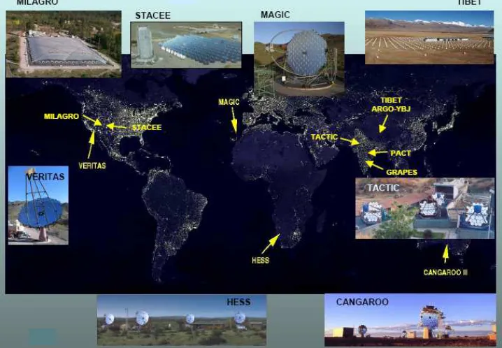
(29) Figure 1.2: Simulated predictions of the one-year all-sky survey of the LAT experiment. launch date is within the next two years, has three instruments, which will cover the energy range from tens of KeV to 50 GeV, being the first satellite that will produce simultaneous detections in the X-ray and γ-ray band. AGILE point source sensitivity is comparable to that of EGRET for on-axis sources and substantially better for off-axis sources, but will have a much larger field of view coverage at energies above 30 MeV (∼ 1/5 of the entire sky), to improve background subtraction. GLAST is a DOE/NASA mission to be launched in September 2007. It will explore the energy range from 30 MeV to 100 GeV with 10% energy resolution between 100 MeV and 10 GeV. The LAT (acronym for Large Area Telescope, the main instruments onboard GLAST) has a field of view about twice as wide (more than 2.5 steradians), and sensitivity at least about 50 times as large, as that of EGRET at 100 MeV, a comparison that improves at higher energies. GLAST will be able to locate sources to positional accuracies from 30 arc seconds to 5 arc minutes, given a much better point spread function, what would allow better searches of counterparts at other frequencies. Figure 1.2 is the simulated GLAST sky after 1 year of survey: several thousand sources are expected to be detected with unprecedented resolution. The LAT instrument onboard GLAST is such that just after 1 day of observations it will detect the weakest of the EGRET sources with 5 σ confidence level. And after 1 week of observations, GLAST will have reached the same sensitivity and coverage than the whole decade of earlier EGRET operations. With a nominal lifetime of five years, and an expected of ten, GLAST will change the perspective of astrophysics in the GeV energy domain in the early 21st century.. 1.2. The experimental status at TeV energies. One of the last challenges of γ-ray astronomy is the distribution of the sources of GeV and TeV photons. Contrary to the lowest energy γ-ray band, photons in this band can be detected using ground-based detectors. To date, almost all the observational results 3.

(30) Figure 1.3: Current ground-based experiments operating in the high energy γ-ray domain. in the energy interval from 100 GeV to 100 TeV have come from observations using the so-called Imaging Atmospheric Cherenkov Technique (IACT). Although considerable effort has been applied to the development of alternative techniques (solar arrays like STACEE (Hanna et al. 2002), air-shower particle detectors like MILAGRO (Atkins et al. 2000), etc.), they are not yet competitive. The window of ground-based γ-ray astronomy was opened in 1989 by the observation of a strong signal from the first TeV γ-ray source, the Crab Nebula, by the Whipple collaboration. The instrument used was the 10 m diameter Whipple Imaging Atmospheric Cherenkov telescope on Mount Hopkins in Arizona. The breakthrough in the technique was achieved by means of the image parameterization suggested by Hillas (Hillas 1985) allowing separation between the rare γ-ray showers and the background from showers induced by charged cosmic rays, which is orders of magnitude more intense. Since then, increasing progress has been made. The old generation of IACTs operating in the 1990s, Whipple, the HEGRA array and CAT, had an energy threshold of several hundreds GeV to several TeV. The turn of the century has brought a new generation of telescopes and arrays of telescopes which are equipped with larger dishes that bring the energy threshold down to ∼100 GeV. The first such instrument was the HESS array (Hinton 2004) of four 12 m diameter telescopes in Namibia. HESS started operation in 2003 and has an energy threshold of about 200 GeV with an unprecedented 5σ flux sensitivity around 0.5% crab for a 50 hour observation. Its angular resolution, around 0.07◦ , and wide field of view turn it into an excellent instrument for sky scans. The 17 m diameter single MAGIC Telescope (Albert et al. 2005a) was commissioned one year later in La Palma, Spain. MAGIC is the lowest energy threshold IACT in the world. It combines a huge ultralight reflector with a large number of technical innovations. The camera has a total field of view of about 3.5◦ . The design of the telescope was 4.

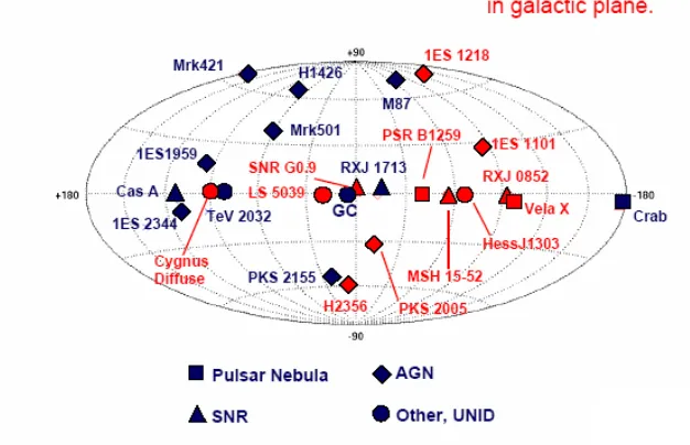
(31) Figure 1.4: Significance map of the H.E.S.S. 2004 Galactic plane scan. 8 high significant sources have been detected. From Aharonian et al. (2005e). optimized for fast repositioning with an eye to perform follow-ups of the prompt emission of Gamma-Ray Bursts (GRBs). Two more telescope systems are well on their way. The VERITAS array (Holder et al. 2005) in Kitt Peak, US, and an upgrade of the existing CANGAROO array (Kawachi et al. 2001) in Australia. Both HESS and MAGIC have recently announced plans for an extension. HESS is to build a gigantic 28 m diameter single telescope at the center of the existing array and MAGIC is already installing a second 17 m telescope to be operated in coincidence with the first one. It will be commissioned in 2007. Figure 1.3 depicts the main ground-based γ-ray experiments nowadays operating world-wide. After the Crab Nebula was established as the standard candle at very high energies (VHE) by Whipple, several years elapsed until the discovery of a second source. Mrk 421, an Active Galactic Nucleus (AGN) was claimed in 1994 again by the Whipple collaboration, that subsequently discovered a second AGN also of the BL Lac type, Mrk 501. The progress was slow during the 1990s. By 2003 the number of confirmed VHE sources had crept up to 12. Thanks to the new generation of IACTs the GeV-TeV astronomy has gone through a phase transition during the last two years. The number of sources has almost tripled. HESS has performed a 112 hour scan (Aharonian et al. 2005e) of the galactic plane in the range of galactic longitude [-30, 30] and ±3◦ latitude. Eight new sources were detected above 6σ (see Figure 1.4) and seven tentative ones above 4σ have been recently released. Four of the eight high significance sources are potentially associated with supernova remnants (SNRs) and two with EGRET sources. In three cases they could be associated with pulsar wind nebulae (PWN). In one case the source has no counterpart at other wavelengths. Along with two other unidentified sources in this energy band, this suggests 5.

(32) Figure 1.5: The Very High Energy γ-ray sky in 2005. Not shown are 8 more sources discovered by HESS in a survey of the galactic plane. Red symbols indicate the most recent detections, brought during 2004 and 2005 by the last generation of IACTs: HESS and MAGIC. From Ong (2005). the possibility of a new class of ’dark’ particle accelerators in our galaxy. Two of the objects in the scan have been recently confirmed by MAGIC (Albert et al. 2005b). Figure 1.5 shows how the number of detected sources in the TeV energy domain has increased in the last two years as soon as the last generation of ground-based Čerenkov telescopes have started operating. The most recent catalogue of sources claims 32 sources, including 6 unidentified objects. There are now two consolidated populations of galactic VHE emitters (PWN and SNRs). The VHE catalogue lists six PWN, six SNRs, one binary pulsar, one microquasar, a region of diffuse emission and eleven AGNs. In the last months MAGIC and HESS have detected several new AGNs with redshifts up to 0.19, at distances almost a factor 10 larger than the two first ones detected at TeV energies.. 1.3. This thesis. Is the aim of this Thesis to focus on one of the multiple astrophysical targets of γ-ray astronomy: the sites of star formation. These extremely active regions are prone of some of the most violent astrophysics phenomena, and thus have been proposed as one of the possible sites for the production of the high energy cosmic rays. However, not many detailed models nor deep high-energy γ-ray observations have yet been devoted to these interesting regions. Is in the better understanding of these regions that this study intends to contribute. The work herein presented is divided in three parts. In the first one, a theoretical and phenomenological approach to both galactic and extragalactic star forming regions is sketched: Chapter 2 investigates the plausibility for the powerful starburst galaxies and ultra-luminous infrared galaxies to appear as a new population of γ-ray sources; Chapter 6.

(33) 3 presents a detailed modeling of the γ-ray emission from the two best candidates from the known extragalactic sites of star formation, looking at them from a multi-wavelength approach; and finally, Chapter 4 proposes that galactic stellar OB associations are possibly detectable TeV γ-ray sources by the current Čerenkov telescopes, without having strong emission at lower γ-ray energies. The second part of the Thesis starts in Chapter 5, summarizing the fundamentals of the Čerenkov technique for γ-ray astronomy and the main characteristics of the MAGIC Telescope; and ends with a description of the analysis applied for the reduction of MAGIC data in Chapter 6. To conclude, the third part reviews the results of the analysis of the first MAGIC observations of star forming regions. Chapter 7 provides the reference analysis of the Crab Nebula data, Chapter 8 presents the upper limits imposed from MAGIC observations to the γ-ray flux of the ultra-luminous infrared galaxy Arp 220, and Chapter 9 reports on the results of the MAGIC observations of the unidentified TeV J2032+4130 source detected by the HEGRA array in the Cygnus region. Finally, Chapter 10 gives some final concluding remarks. This thesis represents the author’s effort to understand a little more about high energy astrophysics in regions of star formation. This effort was threefold. On one hand, technical: participating in the tasks and developments to bring a new Imaging Air Čerenkov Telescope (MAGIC) to work. On the other, theoretical: in order to study what γ-ray output to expect from these regions based on the most detailed possible theoretical models. And finally, observational: in order to begin the long and yet unfinished path to thoroughly test the former predictions. It is here hoped that some of these lines of research will be inspire new developments.. 7.

(34) 8.

(35) Part I. Theory and phenomenology of regions of star formation. 9.

(36) 10.