Computational Models of the
Ventricular Myocardium
PhD Thesis by Ruth Ar´ıs S´anchez
Thesis Director: Mariano V´azquez
Cover Design: Guillermo Mar´ın
Submitted to
Universitat Polit`ecnica de Catalunya
A cardiac computational model is a relevant tool that can give biomedical researchers an additional source of information to understand how the heart works. Numerical models can help to interpret experimental data and provide information about cardiac mechanisms that can not be determined accurately by classical clinical devices. In this thesis, High Performance Computing (HPC) techniques are used to build a cardiac computational tool, which is capable of running in parallel in thousands of processors, allowing high fidelity simulations on fine meshes. To simulate the pumping heart, an explicit coupling scheme between the three-dimensional electrophysiological equations and the solid mechanics formulation is used, solving the governing equations with finite element methods. Also, data assimilation techniques are implemented for the effective estimation of some relevant electrophysiological parameters, which is a crucial step towards the patient-sensitive cardiac model. The data assimilation techniques are assessed on synthetic data generated by the model. Finally, the computational code is applied to simulate real physical problems. The electromechanical propagation in a rabbit geometry is studied to test the sensitivity of the framework to input variations. Particularly, the computational tool is used to evaluate the influence of the fiber field in the contraction of the tissue.
To develop a cardiac simulation useful for clinical purposes, the integrative model requires combining computational mechanics and image processing techniques via data assimilation methods. Coupled with the most advanced image processing analysis, the framework can be the base of theoretical studies into the mechanisms of cardiac pathologies. It can help surgery planning and cardiac modeling, such as the prediction of the impact of pharmacological compounds on the heart’s rhythm or to improve the knowledge of drug study, giving medical researchers additional hints to understand the heart. This realization is only possible in a multidisciplinary team, where specialized groups join forces in their respective disciplines: cardiologists, image researchers,
Els models computacionals del cor s´on una eina important que pot donar als investigadors biom`edics una font addicional d’informaci´o per entendre el funcionament del miocardi. Els models num`erics poden ajudar a interpretar dades experimentals i proporcionar informaci´o complement`aria sobre mecanismes card´ıacs que no poden ser determinats amb precisi´o mitjan¸cant dispositius cl´ınics cl`assics. En aquesta tesi, s’apliquen t`ecniques de computaci´o a gran escala per construir una eina computacional capa¸c d’executar-se en paral·lel en milers de processadors, permetent simulacions d’alta fidelitat en malles fines. Per simular el bombeig del cor, s’utilitza un esquema d’acoblament expl´ıcit entre les equacions electrofisiol`ogiques en tres dimensions i la formulaci´o en mec`anica de s`olids. Per trobar la soluci´o num`erica, s’utilitza el m`etode d’elements finits. A m´es, s’implementen t`ecniques en assimilaci´o de dades per a l’estimaci´o efectiva dels par`ametres electrofisiol`ogics i mec`anics rellevants que apareixen a les equacions, la qual cosa ´es un pas crucial cap a un model card´ıac sensible a cada pacient. El codi computacional s’aplica per simular problemes f´ısics reals. S’estudia la propagaci´o electromec`anica en una geometria de conill, on es prova la sensibilitat del model a les variacions d’entrada. En particular, l’eina de c`alcul s’utilitza per avaluar la influ`encia del camp de fibres card´ıaques en la contracci´o del teixit.
Per desenvolupar una simulaci´o card´ıaca ´util per a fins cl´ınics, el model requereix la integraci´o i combinaci´o de la mec`anica computacional i les t`ecniques de processament d’imatge m´es recents. El model resultant pot ser la base d’estudis te`orics sobre mecanismes de patologies, oferint als investigadors i cardi`olegs pistes addicionals per comprendre el funcionament del cor. Pot ajudar a la planificaci´o de cirurgia i modelitzaci´o, com ´es la predicci´o dels efectes de compostos farmacol`ogics en el ritme card´ıac o l’estudi de l’efecte de medicaments. Aquest projecte nom´es ´es possible en un equip multidisciplinar, on grups especialitzats uneixen les seves forces en les respectives disciplines: cardi`olegs, investigadors imatge, bioenginyers i cient´ıfics de la computaci´o.
CCM Cardiac Computational Modeling
DT-MRI Diffusion Tensor Magnetic Resonance Imaging
EF Ejection Fraction
EM Electromechanics
EnKF Ensemble Kalman Filter
FD Finite Diferences
FEM Finite Element Method
FHN FitzHugh-Nagumo
FK Fenton-Karma
HPC High Performance Computing
LV Left Ventricle
MRI Magnetic Resonance Imaging
ODE Ordinary Diferential Equation
PDE Partial Diferential Equation
PMJ Purkinje Myocardium Junction
ST1 Linear interpolation of rule-based fiber field
ST3 Cubic interpolation of rule-based fiber field
Abstract i
Resum iii
Glossary v
1 Introduction 1
1.1 Motivation . . . 1
1.2 Cardiac computational modeling . . . 3
1.3 Goals of the thesis . . . 9
1.4 Background . . . 12
2 The physical problem: the heart 17 2.1 The cardiac tissue . . . 17
2.1.1 Cardiac electrophysiology . . . 17
2.1.2 Cardiac mechanics . . . 21
2.1.3 The cardiac fiber field . . . 22
2.2 Electrophysiological models . . . 25
2.2.1 The physiological governing equations . . . 26
2.3 Mechanical models . . . 31
2.3.1 Constitutive equations for the cardiac tissue . . . 31
2.4 Electromechanical coupling . . . 34
3.2 Computing the electrical activity . . . 39
3.2.1 Simulation in a biventricular geometry . . . 44
3.3 Computing the mechanical contraction . . . 46
3.3.1 Characterization of the passive stress . . . 47
3.4 Alya . . . 50
3.4.1 Code modularity . . . 50
3.4.2 Strong scalability . . . 53
3.5 Discussion . . . 55
4 Applications of the CCM tool 57 4.1 Fitting of the active force . . . 57
4.2 Relation between conductivity and conduction velocity . . . 60
4.3 Mesh convergence . . . 64
4.4 Effect of the noise in the cardiac fiber field . . . 67
5 Data assimilation. Inverse problem 69 5.1 Kalman filters . . . 70
5.1.1 Kalman filters for linear systems . . . 71
5.1.2 The Ensemble Kalman filters for non-linear systems . . . 72
5.1.3 Non-Linear Application: FHN equation . . . 73
5.1.4 Discussion . . . 79
5.2 Characterization of the cardiac tissue in a human LV geometry . . . 79
5.2.1 Methods . . . 80
5.2.2 Parameter estimation framework . . . 82
5.2.3 Simulation set-up . . . 84
5.2.4 Results . . . 85
5.2.5 Computational remarks . . . 89
6.2 Computational mesh . . . 92
6.2.1 Initial Stimuli . . . 93
6.2.2 Fiber Field . . . 94
6.2.3 Measurements: Volume and Ejection Fraction . . . 96
6.3 Linear rule-based fiber field interpolated in the ventricles . . . 96
6.3.1 Influence of the time-sequence in the activation of the EM wave 100 6.3.2 Density of activation . . . 101
6.4 Cubic rule-based fiber field interpolated in the ventricles . . . 102
6.5 Computational Remark: Parallel efficiency for the coupled EM model . 104 6.6 Discussion . . . 106
7 Conclusions and future work 109 7.1 Contributions . . . 109
7.2 Future lines . . . 112
Bibliography 114
Publications related to the thesis 132
List of figures 135
Introduction
No man-made structure is designed like a heart. Considering the highly sophisticated engineering evidenced in the heart, it is not surprising that our understanding of it comes so slowly.
Daniel D. Streeter
Gross morphology and fiber geometry in the heart.Handbook of Physiology, 1979
1.1
Motivation
Cardiac computational biomechanics studies the use of computers to simulate the heart, converting mathematical models to a code. Different approaches have been used to model the dynamical behavior of biological systems, including mathematical descriptions based on differential equations or cellular automata, which provide a model of the activity of the organ, such as electrophysiology, mechanics or blood flow. In the forefront of cardiac research, the knowledge of the morphology and the functional processes of the heart has a vital interest due to their potential application to the cardiovascular clinics. Experimental studies involving the in-vivo human heart are possible and often available, but they are expensive and very limited. Therefore, well-defined numerical modeling is emerging as a powerful tool that can help to interpret experimental data, allowing the knowledge of phenomena not detectable by classical clinical devices. Simulation can be the base of theoretical studies into the mechanisms
of cardiac pathologies, can provide diagnosis values (Chabiniok et al., 2012) or can be used to assist in therapy planning (Sermesant et al., 2012).
The framework proposed in this thesis aims to create a finite element model of excitation-contraction coupling of the heart based on cardiac data, using the latest advances in image processing and image acquisition. The model is one further step towards the creation of simulations with high precision, which could help to interpret clinical data. The framework could be integrated into medical analysis laboratories where several simulations would be performed on the patient’s data. The results would be delivered to the doctor, who could take decisions on subsequent steps in the treatment: surgery, pacemakers, drugs, stents, etc.
Nowadays, this tendency can be observed in pharmaceutical companies, which already have specialized teams dedicated to mixed simulation and experimental techniques. They are interested in the prediction of the impact of pharmacological compounds on the heart’s rhythm, using computer models, to improve the knowledge of drug study (Staab et al., 2013; Novartis, Novartis). The high performance computational (HPC) simulation tool should lead to a significantly reduction of animal experiments. This also would represent direct savings and reduction in product development for companies.
Creating a simulation of a physiological or pathophysiological process requires knowledge of the process itself. This realization is only possible in a multidisciplinary team, where specialized groups join forces in their respective disciplines. The present work involves medical doctors from several hospitals, image researchers, bioengineers and computational scientists, many of them with the skills extending beyond their core subject of research. This thesis presents the contribution in the project from the Computational Mechanics scientist’s point of view. From this perspective, the issue of understanding how the heart works is amazingly appealing. The development of a HPC-based model of the pumping heart is presented and used to test cardiac properties. The aim is to help researchers and cardiologists to get a deeper insight of the system, and to speed-up our understanding, that “comes so slowly” (Streeter et al., 1969). With this objective, a computational code has been created to represent a new use of HPC resources in biomechanics.
that combines programming flexibility with efficient use of HPC opens a new research perspective.
1.2
Cardiac computational modeling
Cardiac modeling is a complex problem. The maturity of the models of electrical propagation in the heart is still not comparable with the one achieved in other engineering fields. Several causes can explain this difference:
• The heart muscle is a structure composed of cells, whose properties are non-linear, inhomogeneous, time-dependent and anisotropic.
• The biological processes are still partly understood. Direct observations of electromechanical (EM) propagation in the heart tissue is not trivial, and the experimental techniques have strong limitations.
• Experimental validation is still inaccurate and difficult to obtain, when compared to more traditional engineering problems on cars, planes or pumps.
• The problem is extremely multi-disciplinary. To obtain anatomical information and develop the model, the team involves cardiologists, radiologists, image researchers, bioengineers and computational scientists, with all kinds of communication problems among the players.
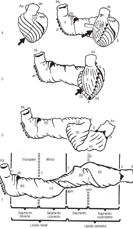
Figure 1.1: Ventricular myocardial band, Torrent Guasp drawing.
developed by Torrent-Guasp et al. (2005). Nowadays this controversial theory is still questioned under differing views.
Under the Computational Mechanics scientist’s point of view, we cannot support any theory, but the development of a ”computational heart” could help to study and assess controversial theories as the helical band.
cell level, EM simulations are based on electrophysiological equations coupled with protein interaction models. Cellular models describe ionic currents and dynamics of the microscopic structures with a high degree of detail. They have been used to describe cellular properties as well as the influence of pharmaceuticals, neurotransmitters and mechanics. Despite all their advantages, it is impracticable to derive a whole heart by modeling every single cell (McCulloch and Huber, 2002).
At organ level, the reaction-diffusion equations describe the spread of the electrical impulse through the myocardium as a continuum. The excitation and electrical propagation process in cardiac tissue is coupled with the mechanical contraction, typically modeled with finite deformation elasticity theory, based on general conservation principles of space, mass and momentum. The present work focuses on the EM simulation of the heart at the continuum level. The code, Alya, is written in parallel, capable of running efficiently in thousands of processors. The starting point is the set of physical models that describe the constitutive parts of the problem. Then, numerical methods are developed to solve the group of non-linear partial differential equations (PDE) that governs the system. In this work, the Finite Element Method (FEM) is used to find the numerical solutions, rendering PDEs into an approximating system of ordinary differential equations (ODE). The FEM includes the 3D geometry, the fiber architecture, electrophysiology, finite strains, non-lineal properties and other features in the analysis. The complete problem can be divided into three parts: the electrical propagation, the mechanical deformation and the blood flowing in and out of the heart. This thesis attacks the first two topics and how they are linked together. The electrical propagation is modeled through non-linear equations representing an excitable media. The deformation is studied as a dynamic large-strain solid mechanics model with an appropriate Ogden-like material. The resultant HPC-based simulation tool provides the coupled EM propagation in cardiac geometries.
Cardiac imaging. To solve numerically electrical and mechanical components, the following anatomical components are used in this work:
• The geometry of the ventricular chambers.
• The definition of the fiber micro-structure.
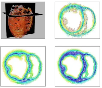
Figure 1.2: Section of the ventricles. Comparison of mathematical model of the fibers (linear and cubic) and experimental DT-MRI in a short cut of the ventricles. Colours represent the angle of the fiber field (from −60◦ on the epicardium to 0◦ at mid-wall
to +60◦).
geometry of the ventricles. MRI is a noninvasive technique that enables accurate descriptions using strong magnetic fields and radiowaves.
Unfortunately, cardiac images of geometry and fiber field are not always available. In those cases, mathematical descriptions are used to define the anatomy, assuming the error that the approximation involves. Figure 1.2 shows three possible orientations of the cardiac fiber field. Linear and cubic models represent mathematical descriptions of the microstructure and DT-MRI represents the experimental acquisition. Based on observations on anatomical dissections in mammalian hearts, those synthetic interpolations describe mathematically the variation of the fibers, from the epicardium to the endocardium. Colours in the figure represent the angle of inclination measured from the wall, typically from −60◦ on the epicardium to 0◦ at mid-wall to +60◦ in the
endocardium.
Mathematical equations modeling the physics of the problem need to be solved in realistic geometries. Moreover, cardiac imaging is continuously improving, there is a wide field of research to remove noise in the acquisitions and to obtain high-resolution recordings. As the quality of the image increases in terms of both signal to noise ratio and spatio-temporal resolution, cardiac accurate models need more computational resources to take profit from this detailed information. Consequently, HPC is a strong tool that can contribute to obtain realistic simulations of the heart using all the information of the detailed data available. The creation of virtual models based on cardiac imaging, using the most recent advances in this field, can be a platform to test new techniques, validate theories, design early clinical trials or predict clinical results.
Data assimilation Electrical and mechanical models that govern the simulation of the heart contain a large number of parameters in their equations, which often cannot be measured directly or that have to be acquiredex-vivo. Although some of them can be found in the literature, a special calibration of these values is required to adapt the simulation to an specific cardiac mechanism.
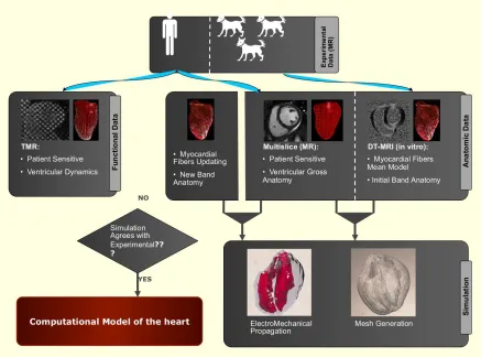
Figure 1.3: Interaction between computational mechanics and image processing techniques. This multidisciplinary project is composed by Hospital de Sant Pau, Centre de Visio per Computador (CVC) and Barcelona Supercomputing Center (BSC). Image designed by Debora Gil (CVC).
Outline of the multidisciplinary project. The HPC-based computational model is a useful tool that can be applied in many multidisciplinary fields. Most of the times, the processing power of computers available to clinical researchers is too limited to simulate physiological and disease mechanisms. In this context, computational scientists are crucial. In the future, the CCM tool presented here aims to cover different clinical disciplines. For example, in pharmaceutical research, the design of HPC-based simulations could improve the time and cost factors in areas such as drug development.
from images and is converted into a computational mesh where the numerical equations are solved. Functional data (cardiac deformation) can be recorded through Cine MRI or ultrasound echocardiography. Both modalities provide reliable measurements of intramural motion that could be used to calibrate the simulation. The resultant simulation of the CCM tool is compared with the experimental 3D motion. Ideally, it should match the observed behavior of the heart. This multidisciplinary project is composed by Hospital de Sant Pau, Centre de Visio per Computador (CVC) and Barcelona Supercomputing Center (BSC).
However, the current technology for reconstruction of 3D motion has a temporal resolution that might not be high enough to produce reliable contractions. Advances in medical imaging have the potential to meet the demands of the requirements of this approach. The improvement of 3D motion is crucial to personalise the cardiac simulation.
1.3
Goals of the thesis
This PhD thesis represents an effort in helping cardiologists to grasp the underpinnings of cardiac dynamics, considering that simulations of biological systems are a complementary tool for physicians to study the organs. The tools developed here should give medical researchers additional hints to understand the heart. The use of numerical simulations in therapeutic applications is in the way of becoming a reality, allowing medical doctors to make decisions on subsequent steps in the patient diagnosis and treatment.
This works aims to investigate some aspects of the mathematical and numerical modeling of the cardiovascular system, focusing on:
• The electrophysiological simulation of the heart
• The mechanical simulation of the heart
• The weak EM coupling
• The HPC-based simulation
is then targeted to biomedical research and based in a general purpose simulation code for coupled multiphysics and programmed for parallel computers. This strategy allows a great flexibility to cover the wide range of problems found in biological systems, being all of them seen in the same way and as any other engineering problem: systems of differential equations coupled together. Alya has no dependency on third-parties libraries, being all solvers developed in-house. The coupled EM solution requires solving electrical and mechanical components, which are performed in the same computational code. The simulation tool is flexible enough to introduce all the necessary modelization improvements, preserving the main features, particularly the scalability. In this thesis, electrophysiological and mechanical models are implemented. The CCM tool is used to test properties of the heart. We analyze its potential on EM cardiac applications through a sensitivity analysis and we present a framework that emphasises the possibility to optimise cardiac models.
Questions and Hypotheses of the work. The work presented here is one of the biomedical problems solved in Alya and means a preliminary step towards the virtual heart simulator. The questions and hypotheses that have been arisen to build and develop the framework are summarized as follows:
• Is HPC necessary?
Computational meshes are commonly used in numerical simulations, offering the advantage of describing the topology and the geometry of the organ as precisely as required. Nowadays, some anatomical data is hard to obtain, for example the orientation of the fiber field in the heart. Since cardiac imaging techniques are improving fast, the newest technology allows to acquire at a high resolution. In the near future, it will increase even more. Therefore, we have to be prepared to use all the information coming from the new medical equipments to consider the increasingly high resolution obtained from the clinical images. High resolution at both geometrical and material levels produce high resolution meshes in the electrical and mechanical problems, which makes high fidelity simulations. HPC is necessary to compute the models of the heart in a fine mesh, which considers all the detail of the geometry that comes from high definition acquisition.
Finally, the electrophysiological, material and coupling models of high complexity have up to a hundred of degrees of freedom per node. If we use complex models in the cardiac simulation, computer resources are also required.
• Why simple electrophysiological models are used in this thesis?
Alya’s flexibility allows to easily program a large variety of physiological models for each problems that needs to be solved. The purpose of this thesis, is to develop an EM propagation of the heart, including the mutual coupling. To simulate the global pumping action, complex models are not required. Models including detailed information of the ionic processes that occur in the contraction of the muscle are suitable for other studies, such as the effect of drugs in pharmaceutical studies. Those models are already implemented in Alya (O’Hara-Rudy, Grandi-Bers) but are not used in this thesis. Instead, Fitz-Hugh Nagumo and Fenton-Karma models are used to run all the simulations.
• Why a fine mesh is needed in the EM simulation of the heart?
In the case of the heart, a fine mesh is necessary to prescribe the anatomical details of the heart available from cardiac images, specially the fiber field orientation. The fiber field information is crucial to develop an EM simulation because it determines the resultant movement of the organ. The orientation of the cardiac fiber field influences the contraction of the heart. Mathematical fiber models can be interpolated in the cardiac geometry when the real data is not available. They are useful and probably suitable to obtain optimal simulations. However, we aim to use the experimental data and all the anatomical description of each case when it is possible.
• Why to solve the electrophysiology and the mechanical deformation of the problem in the same computational mesh?
Electrophysiology and mechanical deformation are solved on the same mesh, with no interpolation. This method allows to avoid stability issues and interpolation errors, paying the price of a high computational cost for the mechanical problem. As all problems are programmed and solved in the same code, supported on the same mesh and with the same parallelization scheme, we find our approach very natural.
• Why to solve both electrical and mechanical problems in the same code?
the model is broader. This also allows improvements and new capabilities to be exploited.
1.4
Background
This thesis focuses on modeling the heart as an organ, based on conservation laws and differential equations that describe the excitation and propagation process in cardiac tissue coupled with the mechanical contraction of the muscle.
The first electrophysiological model was published by Hodgkin and Huxley (1952), where the authors described the dynamics of the transmembrane voltageVm and ionic
currents through the axon membrane. Given the equivalence with cardiac cells, their work on neurons could be used by cardiac scientists to describe the electrical behavior of the heart. A reduction and adaption of Hodgkin-Huxley model to cardiac cells was published by FitzHugh (1961). Due to its simplicity and generality, the FitzHugh-Nagumo (FHN) model has been used widely and is good trade-off for comparisons and simulations (Murillo and Cai, 2004). More complex electrophysiological models have been developed since the late nineteenth century, ranging from single cell (Noble. D, 2001; Ten-Tusscher and Panfilov, 2006), to tissue and organ level (Vigmond et al., 2003; Noble, 2007). Several works have shown how those computational models can be applied to describe 3D phenomena (Penland et al., 2002; Murillo and Cai, 2004; Fenton et al., 2005).
Regarding the simulation of the cardiac contraction, Mirsky (1973) introduced the first model, considering a non-linear problem with great strains and incompressible material. After this first approach, mechanical models incorporated the description of the fiber orientation (Streeter et al., 1969) in the analysis of the stress (Yin et al., 1987). Nowadays, mechanical models account for the anisotropy of the tissue, considering different properties in the planes perpendicular to the fiber direction and through the thickness (Humphrey et al., 1990; Guccione et al., 1991; Costa et al., 1996; Holzapfel and Ogden, 2009). Although the simulation of the contraction in the heart has been studied extensively, there is less published work in the area compared to the electrical modeling.
equations were developed by Hunter and Smaill (1988) and Nielsen et al. (1991). In the last decades, EM models improved quickly in terms of precision and they have been used to investigate pathological phenomena (Cherubini et al., 2008; Niederer and Smith, 2008; Campbell et al., 2009; Keldermann et al., 2010; Trayanova, 2011; Land et al., 2012). Although fully coupled EM modeling is still the exception rather than the rule in cardiac modeling (Trayanova and Rice, 2011), EM simulations have become of increasing use to understand the properties of the heart. Currently, cardiac models are sufficiently accurate to simulate complex processes. In many cases, they have been proved useful for predicting cardiac mechanisms as resynchronization therapy (Kerckhoffs et al., 2009; Constantino et al., 2012; Sermesant et al., 2012), patient-specific applications (Smith et al., 2011; Niederer et al., 2012; Chabiniok et al., 2012; Krishnamurthy et al., 2013) or cardiac growth (Kerckhoffs et al., 2012). The coupled EM problem is significantly demanding in terms of computing (Nickerson et al., 2006). The development of fully coupled 3D solution in large computational domains has been limited due to extremely high computational cost. Particularly, electrophysiology is a more computationally expensive exercise than the mechanical one. Until recently, EM models have been used successfully to study different aspects of cardiac functions, but are made of relatively small meshes. Nowadays, few models are prepared to run on large supercomputers, particularly for the coupled EM case. This lack of resolution is an obstacle when trying to reproduce the complexity of fiber distribution.
Weak coupled models solve the electrophysiology and mechanics problems separately, with only the timing of activation passing between the two systems. The alternative method is the strong coupling between electrophysiology and mechanics, where both systems are solved simultaneously. Up to the author’s knowledge, the groups that develop EM models of the heart at the organ level are summarized here:
• University of California (UCSD). The Cardiac Biomedical Science and Engineering Center has developed a coupled EM model in an anatomical heart geometry to study the effects of pacing on synchrony (Kerckhoffs et al., 2006). They use models that represent the cellular electrophysiology to study the benefit of biventricular pacing in a canine heart, in the presence of left bundle branch block (Usyk and McCulloch, 2003).
• University of Tokio (UT).The UT-Heart Laboratory has developed a multi-scale and multi-physics simulator prepared to perform massively parallel computations. They solve the governing equations of the coupled EM problem, including the ventricular blood flow, using the FEM. The domain is discretized in voxel elements and tetrahedral elements to analyze the electrical and mechanical phenomenon respectively. They apply the simulator on virtual cells and to develop therapeutic devices such as the basic design of an implantable defibrillator (Watanabe et al., 2004; Sugiura et al., 2012).
• King’s College London (KCL). The research group is focused on the development of computational models of the heart with the capacity to integrate multiple measurement types. The multiscale modeling combines detailed cellular dynamics, electrophysiology and deformation models within a common anatomical heart geometry (Niederer and Smith, 2008; Nordsletten et al., 2010).
• IBM Research. The group has developed a code that runs on the Blue Gene supercomputer. They plan to involve higher spatial resolution in the cardiac model.
• INRIA. The M3DISIM team has developed a 3D EM model of the ventricles, using FHN model for the transmembrane potential propagation. The contraction is modeled through a constitutive law including an electromechanical coupling (Sainte-Marie et al., 2006; Sermesant et al., 2012; Chapelle et al., 2012; Caruel et al., 2014). The model enables the introduction of pathologies and the simulation of electrophysiology interventions.
• Stanford University.The Department of Mechanical Engineering has developed a coupled cardiac EM simulation, proposing a fully implicit, FEM-based modular approach (Goktepe and Kuhl, 2010).
• Simula Research Laboratory. The Computational Cardiac Modeling group develops mathematical models of cardiac electromechanics for strongly coupled EM simulations (Sundnes et al., 2014).
• University of Auckland (AU).The team has developed a computational model for cardiac EM which couples cellular, tissue, and whole heart modeling paradigms (Hunter et al., 1997; Nickerson et al., 2006).
myocardial cells and tissue for the development of forces (Seemann et al., 2003). The framework is applied to study the effect of heterogeneity in the EM coupling.
• Politecnico di Milano. The Laboratory for Modeling and Scientific Computing focuses on the development, analysis and computer implementation of mathematical models for the cardiovascular system. The group studies the coupling between cardiac mechanics and electric signal (Ambrosi et al., 2011)
• Zhejiang University, Hanzhou. The group has developed a a unified EM model of the heart at cell level (Xia et al., 2006; Wong et al., 2008). They propose an integrated framework for noninvasive personalization of cardiac electromechanics by combining an integrated cardiac Physiome model and multi-modality observations (Mao et al., 2012).
• Ecole Polytechnique Federale de Lausanne (EPFL), Switzerland The Laboratory of Multiscale Modeling of Materials study the interaction between the propagation of the electrical potential through the cardiac tissue (modeled by bidomain equations), and the mechanical response, assuming a decomposition of the deformation gradient between an active and a passive factors (Rossi et al., 2012).
The physical problem: the heart
In this chapter, a basis about the physiology, structure and mechanical properties of the heart is provided, as well as some of the currently used methods for the acquisition of cardiac data.
2.1
The cardiac tissue
The heart is a muscular organ responsible for pumping blood by repeated and rhythmic contractions. In adult humans, the heart weights approximately 250 to 350 g and is usually situated in the middle of the thorax. It is composed of semi-striated muscle that functions by contraction, causing the muscle cells to shorten. It contracts 72 beats per minute.
2.1.1
Cardiac electrophysiology
The wall of the heart has three layers: Theepicardium,myocardium andendocardium. Endocardium and epicardium are thin layers consisting primarily of collagen and elastic tissue. In the middle layer, the myocardium, the cells that constitute the muscle show electrical excitability. These specialized cells, called myocytes, are organized into parallel cardiac fibers giving the muscle the striated appearance. The fibers form sheets which are connected one to another by collagen (Fung, 1993), (Fig. 2.1).
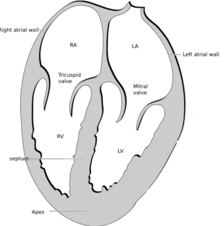
Four chambers can be distinguished in the heart: two atria and two ventricles (Fig. 2.2). The interatrial septum is the wall that separates the right and left atria of the heart and the interventricular septum separates the ventricles.
Figure 2.1: Sections of cardiac muscle. Heart wall showing the pericardium, myocardium and endocardium (left). Cardiac fibers give a striated aspect to the myocardium (right). Image by Stephen Gallik.
The valves of the heart are located within the chambers, preventing the back flow of blood. The tricuspid valve is placed between the right atrium and right ventricle and the mitral valve is situated between the left atrium and the left ventricle. Right ventricle (RV) pumps blood to the lungs for oxygenation through the pulmonary artery. Left ventricle (LV) pushes blood into the aorta to deliver it to all the body tissues, pumping blood at a higher pressure than the RV.
The action potential. A cardiac cell (myocyte) is typically 10 to 20µm in diameter and 80 to 125 µm in length. The cell membrane acts as an electrical insulator and contains ion channels which transport electrical current by diffusion. The potential difference across the membrane is called transmembrane potential. Initially, a cardiac cell is at rest, with a potential difference across the membrane. The potential inside the cell is negative compared to the external. If the membrane potential rises to a certain threshold value (close to 40 mV) a rapid process occurs, which can be explained in different phases:
Figure 2.2: Longitudinal cut of the heart showing the four chambers. Illustration by CC Patrick J. Lynch and C. Carl Jaffe, Yale University, 2006.
• Depolarization: An excitation opens the fastN a+channels, causing a large influx of ions through the membrane and rapid increase of conductance to these ions. The cell changes its potential becomingVmax less negative.
• Early repolarization: Inactivation of the fastN a+channels. A current ofK+ tries to recover the equilibrium of the action potential to the resting state.
• Plateau: There is a balance between an inward movement of Ca2+ and the outward movement of K+.
• Repolarization: Ca2+ channels close while K+ channels are still open. The cell loses its positive charge and causes the cell to repolarize.K+channels close when the membrane potential is restored to -85 mV.
The charge is transported by the ionic currents and is accumulated at the membrane (Fig. 2.3). The complete cycle of depolarization and repolarization is called action potential and is illustrated in Figure 2.4.
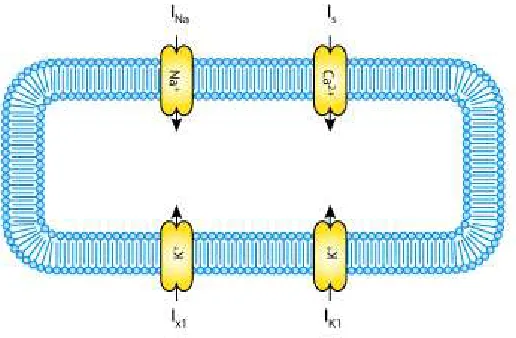
Figure 2.3: Schematic diagram describing the current flows across the cell membrane. From the CellML Project.
[image:32.595.90.467.423.654.2]Figure 2.5: Illustration of the heart muscle showing the sinoatrial (1) and atrioventricular (2) nodes and the Purkinje system. By CC Patrick J. Lynch and C. Carl Jaffe, Yale University, 2006.
actin and myosin proteins in the intracellular domain. The myocytes generate an active tension making the cell to shorten.
Purkinje system. The electrical signal that triggers contraction enters from the atrioventricular node to the bundle of His. This bundle branches out into a tree-like structure called Purkinje fibers, which provide rapid delivery of the electrical impulse (Fig. 2.5). Purkinje system and myocardium muscle are electrically connected through transitional cells called myocardium junctions (PMJs), distributed throughout the ventricular subendocardial layer.
2.1.2
Cardiac mechanics
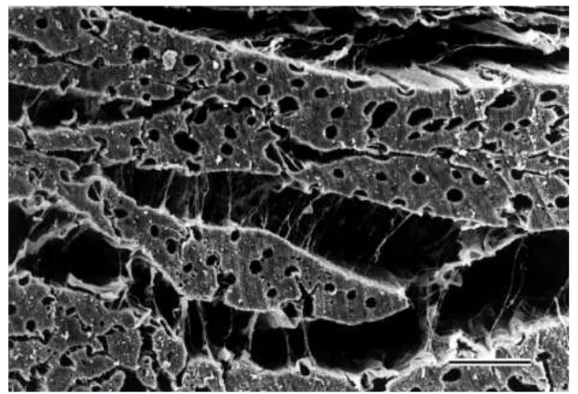
Figure 2.6: Scanning electron microscopy of the myocardium sectioned perpendicular to the fibers (Legrice et al., 2001). Fibers, muscle bridges and collagen are visible.
(Fung, 1993; Yin et al., 1996; Humphrey, 2001). Taking into account the behaviour of the myocardium, the stress of the muscle is divided in two parts:
• The active stress represents the active component of the embedded muscle fibers. The active part is generated by the contractile cells when they are electrically stimulated.
• The passive part represents the contribution of the surrounding matrix of connective tissue, mostly collagen and elastin.
2.1.3
The cardiac fiber field
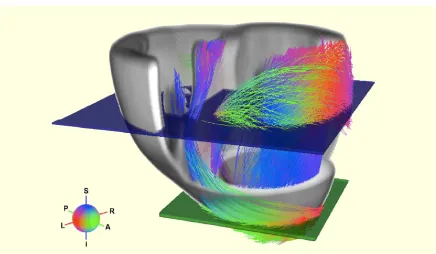
Figure 2.7: Representation of the cardiac fiber field (Peyrat et al., 2006).
mathematical models have been constructed, integrating the fiber orientation. In these synthetic cardiac structures, the angle varies from base to apex across the wall (i.e. transmural), from −60◦ to −70◦ in the epicardium to 60◦ to 70◦ in the endocardium
(Fig. 2.7).
fields over the whole myocardial volume, image-based and rule-based methods. The main characteristics of experimental and synthetic fiber models are presented here:
Diffusion Tensor Imaging. In recent years, Diffusion Tensor Magnetic Resonance Imaging (DT-MRI or DTI) has emerged as a powerful tool for the experimental measurement of cardiac fiber structure. This method is based on the assumption that water diffuses along the myocardial fiber orientation. Applying magnetic field gradients in at least 6 directions in the cardiac sample, it is possible to calculate a tensor T
that describes the 3-dimensional shape of the diffusion. This matrix is symmetric and positive. The eigenvalue decomposition leads toT =P DPT, wereP is the eigenvectors
matrix and D the diagonal matrix of the eigenvalues. The eigenvalues of the diffusion tensor quantify the diffusion rate of water molecules within the tissue structure along the directions given by the corresponding eigenvectors. Finally, the fiber direction is indicated by the tensor’s main eigenvector.
DT-MRI is a non-invasive technique which allows a direct measurement of the anisotropy (Basser et al., 1994). However, DT-MRI data is noisy and the quality of the reconstructed images is related with the number of DT-MRI acquisitions. An average model can be obtained combining reconstructions of the same heart sample, giving better quality to the distribution. Up to date, a full 3D DT-MRI acquisition of the fiber data requires extremely long times to achieve the minimal accuracy for the reconstruction (several hours) and can only be performed on ex-vivo hearts (Helm et al., 2005). Novel studies in 2D show that the acquisition of high resolution in-vivo is becoming feasible (Gamper et al., 2007; Toussaint et al., 2010, 2013; Harmer et al., 2013). Due to cardiac motion, the acquisition of high resolution
in-vivo DT-MRI is a challenging task. In the near future, the improvement of this technique will lead to a simulation of the human heart including the anatomy and the anisotropic structure of the human organ, both acquired in-vivo.
Rule-based fiber models. The experimental fiber field is not always available. For this reason, rule-based models describing the cardiac fibers are frequently used. Based on experimental measurements such as in Streeter et al. (1969), the fiber orientation is generated by mathematical algorithms. Rule-based models are validated comparing to those in the same geometrical model but with DT-MRI-derived fiber orientation.
calculated (dendo, depi). The transmural variation of the fiber field is represented from−θ
on the epicardium to 0 at mid-wall to +θon the endocardium, by using the epicardium to endocardium surface distanced. The value of θ usually varies between 60◦ and 70◦.
A thickness parameter is defined as
e= dendo
dendo+depi
(2.1)
The interpolation of the fiber along transmural direction is defined as
θ=R(1−2e)n (2.2)
where R=π/3 for the LV and R =π/4 for the RV.
This approach has shown some success in ventricular models with basic geometries (Potse et al., 2006; Bishop et al., 2010). However, minimal distance parametrization can yield to singularities in the minimal distance function in realistic geometries, particularly in the septum (Bayer et al., 2012). The advantages of synthetic fiber field models are:
• Fast algorithm and fast implementation
• Fiber direction can be modified to examine its effect in propagation
• New fiber models can be incorporated
• Long acquisitions required to acquire in-vivo fiber data are avoided
Moreover, new studies present a method to personalize the fiber architecture. Based on inverse techniques as the Unscented Kalman Filter, the parameters of the rule-based fiber model are estimated from DT-MRI-derived fiber data (Nagler et al., 2013).
2.2
Electrophysiological models
At the organ level, reaction-diffusion systems reproduce continuous approximations of the excitation of cardiac muscle (Hunter, 1983). Nowadays, two models are widely used in electro-cardiology to simulate the propagation of the action potential waves in the cardiac tissue: the bidomain and monodomain models.
The bidomain model. It represents a well-established description of the electrical activity of the myocardium on a macroscopic scale, taking into account the ionic current, the membrane potential and the extracellular potential. In the bidomain model, the simulation of the ionic current requires the solution of a system of partial differential equations (PDE’s), with an implicit analysis. The model considers that the muscle cells are connected via small channels in the cell membrane, where substances such as ions pass directly from one cell to another.
The model is suitable for problems that require ion exchange calculations, such as the study of defibrillation or induced arrhythmia in small samples of cardiac tissue (Trayanova et al., 2006). In these applications, the bidomain model captures the tissue behavior.
The monodomain model. The monodomain model is a simplification of the bidomain equations. It assumes that conductivities are proportional in the intracellular and extracellular spaces. The advantage of the model is that it produces realistic activation patterns, useful for analysis and simplified electrophysiological studies. Depending on the purpose of the study, the monodomain model is accurate enough to simulate the action potential (Sundnes et al., 2006; Potse et al., 2006). However, it cannot be applied in all situations because it does not permit currents in the extracellular domain.
2.2.1
The physiological governing equations
Hodgkin and Huxley (1952) introduced the first continuous mathematical model designed to reproduce cell membrane action potentials. Since then, there has been many complex models developed for cardiac cells following their approach. In general, the action potential V(xi, t) is modeled using a reaction-diffusion equation through a
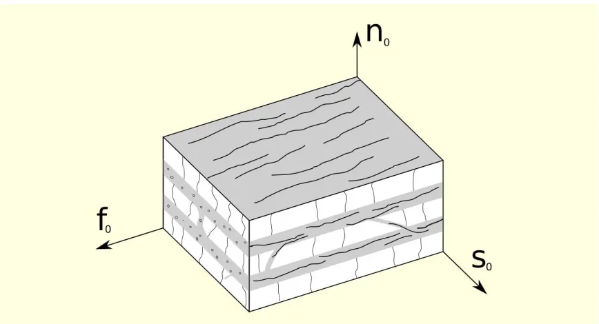
Figure 2.8: Local coordinate system. Fiber (f0), normal (n0) and sheet (s0) directions are drawn.
form of the electrical propagation equation is1:
∂Vα
∂t = ∂ ∂xi
Dij
∂Vα
∂xj
+L(Vα). (2.3)
Greek subindices label the number of tissue domains. In the case of monodomain models
α = 1. For bidomain models α = 1,2, representing the extracellular and intracellular potentials (Simelius et al., 2001). On the right hand side of the equation two terms can be distinguished:
1) Diffusion term: It is governed by the conductivity tensor Dij, which represents
the conductivity in the axial and crosswise fiber direction. At a given point, a set of perpendicular unit vectors is defined: f0 is the unit vector along the cardiac fiber at the given point,n0 is perpendicular to the fiber in the sheet plane and s0 is normal to the sheet plane (Fig. 2.8). The conductivity tensor Dij in 2.3 is written as:
Dij =Cik−1 D
loc
lk Clj, (2.4)
where Cij is the transformation matrix with respect to the local basis {f0, no, s0}. Expressed in the basis formed by these three vectors, the local conductivity tensorDloc
lk
is diagonal:
D=
kf 0 0
0 ks 0
0 0 kn
(2.5)
whose diagonal components are the axial and crosswise conductivities. As reported in (Clerc, 1976; Rubart and Zipes, 2001; Coghlan et al., 2006), the conduction velocity is three times faster in the direction of the long axis of myocardial fibers than in a direction perpendicular to this long axis. Supposing the same relation, the crosswise conductivity is then one third of the axial conductivity (kf = 3kn= 3ks).
2) Non-linear term: L(Vα) is the non-linear operator representing the total
membrane ionic current Iion and the applied stimulus Iapp. For the Iion current, different models reproduce the process of cardiac activation and deactivation. They are commonly grouped into three categories:
• Phenomenological models.Simplified models that use the minimum set of currents necessary to reproduce macroscopically observed behavior of cells, such as the action potential (FitzHugh, 1961; Fenton et al., 2005). These models are numerically efficient but they are not able to identify cardiac mechanisms.
• 1st generation ionic models. They reproduce basic ionic currents and concentrations (Beeler and Reuter, 1977; Luo and Rudy, 1991).
• 2nd generation ionic models. They give a direct description of ionic currents and concentrations and they reproduce an accurate shape of the action potential (DiFrancesco and Noble, 1985). They are robust models but numerically expensive.
The type of the ionic model Iion is chosen depending on the application of the study. Simple models are suitable to simulate the pumping heart in macroscopic situations, where a detailed description of the mechanisms in the cell membrane is not necessary. On the contrary, complex ionic models are used to study cell processes. For example, pharmaceutical studies demand the modeling of the ionic exchange in the cell membrane. In this case, the evolution of the electrical wave without a detailed description of the mechanisms in the cell membrane would not be enough to capture the effect of drugs in the electrical propagation.
-120 -100 -80 -60 -40 -20 0
0 20 40 60 80 100 120 140 160 180 200 220
Transmembrane potential [mV]
[image:41.595.150.449.99.314.2]Time [ms]
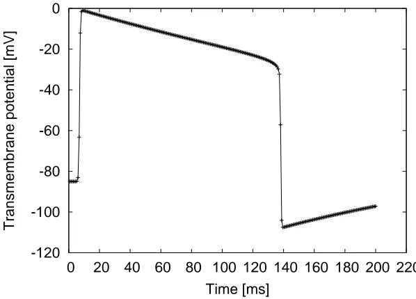
Figure 2.9: Fitzhugh-Nagumo transmembrane potential, temporal evolution for a given position.
Fitzhugh-Nagumo. Based on observations, Fitzhugh-Nagumo (FHN) is a generic model for excitable media (FitzHugh, 1961). It is a simplification of the Hodgkin-Huxley equations and does not include a physiological description of the ion exchange in the cell membrane. Although the model does not account for realistic ionic processes and concentrations, it is able to reproduce the macroscopic behaviour of excitable cells. The most general properties of the myocytes are reproduced using two variables: the transmembrane potential (V), and the recovery potential (w), which is introduced to simulate the repolarization of the cell. The equations of the model are the following:
Iion = c1V(V −c3)(V −1) +c2w
∂w
∂t = ε(V −γw) (2.6)
Constants c1, c2 and c3 define the shape of the propagation wave and ε and γ control the recovery potential evolution. The action potential generated by the FHN model is shown in Figure 2.9. Although the shape is mathematically obtained and it is not based on cellular changes, the propagation of this electrical wave permits to investigate macroscopically how changes in the electrical activation affect the function of the muscle tissue.
-100 -80 -60 -40 -20 0 20
0 20 40 60 80 100 120 140 160 180 200 220
Transmembrane potential [mV]
[image:42.595.130.427.99.313.2]Time [ms]
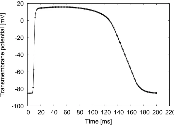
Figure 2.10: Fenton-Karma transmembrane potential, temporal evolution for a given position.
contains three ionic currents, corresponding to sodium, calcium, and potassium (Fenton and Karma, 1998). The total membrane currentIionis given by the sum of the
three phenomenological currents Jfi, Jso and Jsi. The first one, Jfi is analogous to the
N a+ current related to the depolarization of the membrane. Secondly, J
so represents
the K+. Finally, J
si is comparable to the Ca2+ current, and triggers the contraction
of the cardiac tissue. FK equations use three variables: the transmembrane potential
V and two ionic gates v, w. For each current and for each ionic gate one equation is computed:
Iion = Jfi(V,v) +Jso(V) +Jfi(V,w)
∂w
∂t = Θ(Vc−V)
(1−w)
τ− w
− Θ(V −Vc)
w
τ+
w
∂v
∂t = Θ(Vc−V)
(1−v)
τ− v
− Θ(V −Vc)
v
τ+
v
Jfi(V,v) = −
v
τd
Θ(V −Vc)(1−V)(V −Vc)
Jso(V) =
V τ0
Θ(Vc−V) +
1
τr
Θ(V −Vc)
Jsi(V,w) = −
w
2τsi
(1 + tanh[k(V −Vsi
where Θ is the Heaviside function. Depending on the choice of the model parameters, the FK mimics Beeler-Reuter or Luo-Rudy models (Fenton and Karma, 1998). The action potential generated by the model is shown in Figure 2.10. The shape of the transmembrane potential V is obtained mathematically and reproduces a softer potential evolution than in the FHN case.
In this work, FHN and FK models are used to reproduce the most important characteristics of the action potential.
2.3
Mechanical models
The response of the cardiac tissue is characterized by a constitutive equation which gives the stress as a function of the deformation of the heart. The constitutive relations allow us to mathematically define the characteristics of the cardiac muscle.
Initially, mechanical models described the myocardium as isotropic (Demiray, 1976). Later, tests in the fibers of canine hearts showed that the myocardium has a significant anisotropy with a stiffness substantially bigger in the fiber direction than the orthogonal cross-fiber direction (Yin et al., 1987). To account for the anisotropy of the cardiac tissue, transversely isotropic models where introduced considering the same physical properties in the planes perpendicular to the fiber direction but different properties through the thickness (Humphrey et al., 1990; Guccione et al., 1991; Costa et al., 1996). This version of the law is useful when the fiber field is only characterised by its direction, with no information on their eventual sheet-like grouping. However, experimental tests performed on excised slices of cardiac muscle revealed that the tissue presents a particular orthotropic-layered architecture, meaning that the mechanical properties are different along the axis determined by the fiber orientation (Novak et al., 1994; Dokos et al., 2002). One of the first works in orthotropic constitutive models was developed by Hunter et al. (1997), containing 18 parameters in the equations. Recently, a locally orthotropic constitutive model was introduced by Holzapfel and Ogden (2009), using fiber-based material invariants.
2.3.1
Constitutive equations for the cardiac tissue
chosen to model the cardiac muscle (Watanabe et al., 2004; Dorri et al., 2006). The constitutive equations presented here are a transversally isotropic version of the orthotropic law described by Holzapfel (2000).
Governing equations. Consider Ω0 as a fixed reference configuration of a body and Ω the deformed one. The position vector of a particle in the body is expressed in this work by Xi in the first configuration and by xi in the second one (note that
capital letters and subscripts are used for scalars or tensors defined in the reference configuration, and lowercase letters and subscripts when defined in the deformed configuration). Being the displacementui =xi−XI, the relation between both measures
is given by the deformation gradient:
FiJ =
∂xi
∂XJ
=δiJ +
∂ui
∂XJ
(2.8)
In a total-Lagrangian formulation, results are referred to the initial state. The governing equations are written as:
ρo
∂2ui
∂t2 = ∂PiJ
∂XJ
+ρoBi (2.9)
where ρo is the initial density of the body, Bi is the body force and PiJ is the first
Piola-Kirchoff stress tensor. Being J the determinant of the deformation gradient F, the Cauchy stress tensor is related to the first Piola-Kirchoff stress as follows:
σ =J−1P FT (2.10)
Suppose a compressible, homogeneous, hyperelastic material. The constitutive behavior of such material is expressed in terms of a strain energy function W and the right Cauchy-Green deformation b =F FT
:
σ = 2J−1∂W(b)
∂b b (2.11)
It can be useful to develop general expressions of stress in terms of the strain invariants ofb. The invariants are of particular interest when developing constitutive laws because they remain unchanged when expressed in a different basis. The three first invariants of b are:
I1 =trb, I2 =
(trb)2 −trb2, I
3 =det(b) (2.12)
coincides with the muscle fiber orientations. The mean fiber orientation is represented byf0. The sheet axis that lies in plane perpendicular to the fibers iss0 and n0 is the
normal to the plane formed by the two other vectors. If the material is modeled as transversally isotropic, the fourth strain invariant will be needed:
I4 =f0bf0 (2.13)
Using the chain rule,
∂W(b)
∂b = X
α
∂W ∂Iα
∂Iα
∂b (2.14)
and the definitions of the strain invariant derivatives (Eq. 2.11) is reformulated as follows Holzapfel and Ogden (2009):
σ= 2J−1W
1b+ 2J−1W2(I1b−b2) + 2JW3I + 2J−1W4f ⊗f (2.15) where the notation Wi =
∂W ∂Iα
and f = F f0. This notation is used to underline the
fact that f is not a unitary vector. Based on physiological considerations, a form of
W is suggested in Holzapfel and Ogden (2009). The energy function for the reduced transversally isotropic version presented here is given by
W = a 2be
b(I1−3)− a
2(I1−3) +
af
2bf
n
ebf(I4−1)2
−1o+ K
2 (J −1)
2 (2.16)
The strain-energy function represents the change of the material properties during the activation. The volumetric energy term function of J have been added to make the material compressible. Introducing the expression of the derivatives of the energy in the general stress equation gives the following:
Jσpas = (a eb(I1−3)−a)b+ 2af(I4−1)ebf(I4−1)
2
2.4
Electromechanical coupling
Electro-mechanic: Macroscopically, the excitation-contraction coupling is the phenomenon by which the fibers contract after a wave of electrical activation propagates through the myocardium. A large amount of EM coupling models have been developed (Rice and de Tombe, 2004). A ’one-way coupling’ model is presented in this work, considering that the displacements have no influence on electrophysiology. The total Cauchy stress is developed in two parts, active and passive (Humphrey, 2001):
σ =σpas+σact(λf,[Ca2+])f ⊗f (2.18)
The passive part is governed by a transverse isotropic exponential strain energy function
W(b), defined in Equation 2.16. The active part is calculated as in Holzapfel (2004). It is assumed to be produced in the direction of the fiber. If the muscle fiber stretch is represented by λf, the excitation-contraction coupling is modeled as follows:
σact=γ
[Ca2+]n
[Ca2+]n+Cn
50
σmax(1 +β(λf −1)) (2.19)
In this equation, Cn
50, σmax and β are model parameters. The coupling parameter γ is
used to graduate the active stress (0 < γ < 1). The concentration [Ca2+] mediates the contraction of the myocardium and fluctuates in time following this relation (Hunter et al., 1998):
[Ca2+](tloc) = [Ca2+]max(tloc/τCa)e(1−tloc/τCa) (2.20)
where τCa is a parameter and tloc is the local activation time. The tloc is initiate to 0 s
at the beginning of the simulation for the entire mesh. When the membrane potential overcomes a threshold value (fixed to -5 mV), EM coupling is triggered andtloc starts
running at this specific location. Then, [Ca2+] (and consequently σ
act) also vary.
Figure 2.11 shows the relation between the local activation time and the action potential, the concentration of intracellular [Ca2+] and the normalized active force produced. Parameter values are Cn
50 = 0.5µm, σmax = 100kP a, β = 2.5,[Ca2+]max =
1.0µm, n = 3 and τCa = 0.06s. In this problem, the electrical propagation is
solved using a monodomain model and a FHN ionic current model. The electrical conductivity is isotropic, equal to 0.012 ms/cm and the membrane capacitance is
-110 -75 -50 -25 0
0 0.05 0.1 0.15 0.2 0.25 0.3 0.35 0.4
0 0.2 0.4 0.6 0.8 1 1.2
E (mV)
[Ca
++
] (
µ
M)
time (sec)
[image:47.595.136.471.99.338.2][Ca++] Membrane potential Normalized active force
Figure 2.11: Time scale comparison of the normalized active force, the membrane potential and the [Ca2+].
Mechano-electric: The algorithms of continuum mechanics usually make use of two classical descriptions of motion: the Lagrangian description and the Eulerian description (Donea et al., 2004). In a Lagrangian description, the computational mesh follows the movement of the body. Each node of the mesh coincides with the associated material particle during motion. In the Eulerian description, the computational mesh is fixed and the body moves with respect to the grid.
HPC cardiac computational
modeling
Working at the organ-level, the cardiac computational model requires solution of three components: the electrical signal, the mechanical deformation and the excitation-contraction coupling that links both problems together. The equations of the complex models describing the heart can not be solved analytically, they must be solved on a computer using numerical techniques.
The main topic of this chapter is the solution of the governing equations to simulate the electromechanical propagation of the heart. The methods are based on a finite element approach (FEM), focusing on the solution in parallel computers. The time evolution of the system is calculated using an Euler scheme. We also present and analyze two different integration rules in the right hand side of the equation that solves the problem, with and without mass lumping. We underline the most remarkable differences between them.
Finally, the computational code Alya is presented. The tool is used in this thesis to run cardiac simulations, solving both cardiac electrophysiology and mechanics. Alya is conceived as a multiphysics platform to deal with coupled computational problems in parallel, designed from scratch to take profit of parallel architectures with parallel efficiency.
Figure 3.1: Canine ventricular data, Johns Hopkins University. MRI data is processed to obtain the computational mesh. Green dots correspond to the voxels obtained from the image. The geometry is discretized in tetrahedral elements, using the mesh generator Tetgen. A slice of the ventricular mesh is represented in colours.
3.1
The computational domain
To solve the electromechanical problem, the typical domain in this project is a 3D cardiac geometry consisting in two ventricles. Figure 3.1 shows an anatomically detailed MRI-derived canine ventricular model developed by Johns Hopkins University. The continuous volume, extracted from cardiac images, is divided into small elements and the governing equations are numerically solved within these elements. In 3D, the FEM-based space discretization allows different element types to solve the governing equations. Particularly, the cardiac geometry can be divided in tetrahedral or hexahedral elements. After some tests, tetrahedra have been chosen to solve the large-scale problems in this work because they fit anatomical information obtained from clinical images. Given the increasing resolution and accuracy of cardiac imaging, unstructured tetrahedral meshes can be easily adapted to complex geometries and can be efficiently generated from raw data.
3.2
Computing the electrical activity
Cardiac electrophysiology is modeled here at the organ level. Considering a monodomain scheme, the parabolic reaction diffusion equation can be written as follows: Cm ∂V ∂t = ∂ ∂xi Dij Sv ∂V ∂xj
+L(V), (3.1)
where Cm is the membrane capacitance (µF cm−2) and Sv is the surface to volume
ratio. The non linear term L(V) represents the total membrane ionic current is Iion and the applied stimulus Iapp (µA cm−2).
To find the value of the action potential V, the discretization of the partial differential equations is carried out using a variational formulation (Johnson, 1987). Assuming that the solution V belongs to the the usual FEM interpolation function space V, the test function ψ ∈ V is chosen (Eriksson et al., 1996). The simulation domain is Ω and its boundary is ∂Ω. The weak form of Equation 3.1 is obtained by first multiplying by
ψ and then integrating over the domain Ω. Three terms can be distinguished in this equation:
Z
Ω
ψ∂V ∂t dΩ
| {z }
Mass term = Z Ω ψ ∂ ∂xi Dij
CmSv
∂V ∂xj
dΩ
| {z }
Difussion term
+ 1
Cm
Z
Ω
ψL(V)dΩ
| {z }
Non-Linear term
(3.2)
1) Mass term: Corresponds to the time derivative term.
2) Diffusion term: Using the chain rule and the Gauss’s theorem, the diffusion term gives:
Z
∂Ω
ψ Dij CmSv
∂V ∂xj
njdS−
Z
Ω
Dij
CmSv
∂ψ ∂xi
∂V ∂xj
dΩ (3.3)
The first part of the diffusion term is used to impose Neumann boundary conditions. To a first approximation, the fluxes on the boundaries are set to zero, and this part vanishes. No Dirichlet conditions are directly imposed.
Linearizing the ionic equation, L(V) can be expressed as:
L(V) = c1V(V −c3)(V −1) +c2 ≡V f(V)
∂w
∂t = ε(V −γw) (3.4)
Rewriting the three terms in the weak form, the system to be solved is:
Z
Ω
ψ ∂V
∂t dΩ = −
Z
Ω
Dij
CmSv
∂ψ ∂xi
∂V ∂xj
dΩ + 1
Cm
Z
Ω
ψ V f(V)dΩ
∂w
∂t = ε(V −γw) (3.5)
Discretization in space. The spatial discretization of Equation 3.5 is performed using a FEM approach. The solution V and its derivative are expressed as:
V(x, t) =
nnodes
X
k=1
ψk(x)Vk(t)
˙
V(x, t) =
nnodes
X
k=1
ψk(x) ˙Vk(t) (3.6)
Introducing these expressions, the Equation 3.2 yields:
˙
V
Z
Ω
ψiψj dΩ =−V
Z
Ω
∂ψi
∂xi
Dij
CmSv
∂ψj
∂xj
dΩ +V f(V) 1
Cm
Z
Ω
ψiψj dΩ (3.7)
After discretization, Equation 3.5 can be expressed in a matrix form:
MV˙ = −KV +M Vf(V) ˙
W = ε(V −γW) (3.8)
The FEM-based formulation leads to a mass matrixM in the time derivative term, a diffusion matrix K, with anisotropic diffusion tensor, and a non-linear ODE-like term for the IIon current.
Figure 3.2: Integration rules for triangles. Open rules with one or three integration points and one closed rule with three integration points.
other complex models would permit the implicit solution just in the diffusion term, not in the non-linear term Ten-Tusscher and Panfilov (2006).
The temporal discretization of the equation is performed using the FD method. Then, the derivatives of V and W are expressed as:
˙
V = V
n+1−Vn
∆t
˙
W = W
n+1−Wn
∆t (3.9)
where ∆t is the time step, Vn is the solution at the current step and Vn+1 is the solution at the new time step. Using an explicit Euler scheme, the matrix form yields:
M ∆tV
n+1
= M
1
∆t +f(V
n
)
Vn
+KVn
Figure 3.3: Anisotropic 2D potential propagation sequences: closed integration rule for the ODE-like term (top) versus open integration rule for the ODE-like term (bottom). The first option gives the proper shape and propagation speed.
• Theopen rule, where the integration points are not coincident with the nodes. In this case,M is called consistent matrix and is not diagonal. A special treatment of the rows is performed to diagonalize it.
• Theclosed rule, where the integration points are coincident with the nodes.M is called lumped matrix and is diagonal. Nodal locality is preserved because shape functions are built by setting them to one in its own node and zero in the rest of them.
Mass lumping is a numerical technique related to the FEM that has been widely used in different applications. Figure 3.2 shows three integration cases for triangles, where the open and closed rules are used.
To compare the results of the open and closed numerical integrations, the electrical propagation equations are solved in a 2D anisotropic media, with cardiac fibers oriented in horizontal direction (Fig. 3.3). FHN model is used to simulate the evolution of the action potential through the cardiac tissue. In this simulation, conductivities in Cartesian axes are chosen proportional (kx = 3ky). The figure shows a sequence of the
-100 -80 -60 -40 -20 0 20
0 20 40 60 80 100 120 140 160 180 200
V (mV)
t (ms)
[image:55.595.150.455.97.313.2]Lumped No Lumped
Figure 3.4: Action potential with open and closed integration rules: speed differences for the closed rule (“lumped”) and the open rule (“no-lumped”) used in the ODE-like term.
the non-linear term in the ODE. Top row corresponds to lumped or closed integration rule and bottom row corresponds to the consistent or open rule. The use of the open rule introduces a significant error in speed and propagation behavior. The difference in speed between the two models can be observed in Figure 3.4. The open rule (green curve, called “no lumped”) produces a propagation that arrives earlier than the closed rule (red curve, called “lumped”). Apparently, consistent matrix leads to higher cross-diffusion.
Finally, Figure 3.5 shows the results when the diffusion term is set to zero. In case of no diffusion, the action potential should not propagate through the cardiac tissue. If the governing equations are integrated using the open rule, an artificial numerical diffusion is introduced producing a wrong propagating behavior . On the contrary, when the closed rule is chosen, the initial condition does not propagate, as expected.
Critical time step. The typical procedure to solve transient problems explicitly is to compute a local time step at each mesh element using its characteristic size h