Grasp plannind under task-specific contact constraints

U

NIVERSITAT

P

OLITÈCNICA DE

C

ATALUNYA

Programa de Doctorat

AUTOMATIZACIÓ AVANÇADA I ROBÒTICA

Tesi Doctoral

G

RASP

P

LANNING UNDER

T

ASK

-

SPECIFIC

C

ONTACT

C

ONSTRAINTS

Carlos J. Rosales Gallegos

Directors:

Lluís Ros Giralt and Raúl Suárez Feijóo

Institut d’Organizació i Control de Sistemes Industrials

Programa de doctorat:

Automatizació Avançada i Robòtica

Aquesta tesi ha estat realitzada a:

Institut de Robòtica i Informàtica Industrial, CSIC-UPC Institut d’Organizació i Control de Sistemes Industrials, UPC

Dirigida per:

Lluís Ros Giralt and Raúl Suárez Feijóo

Realitzada per:

Carlos J. Rosales Gallegos

Compartida segons:

Creative Commons License Attribution-NonCommercial 3.0

G

RASP

P

LANNING UNDER

TASK-

SPECIFIC

CONTACT

CONSTRAINTS

Carlos J. Rosales Gallegos

Abstract

Several aspects have to be addressed before realizing the dream of a robotic hand-arm system with human-like capabilities, ranging from the consolidation of a proper mechatronic design, to the development of precise, lightweight sensors and actuators, to the efficient planning and control of the articular forces and motions required for interaction with the environment. This thesis provides solution algorithms for a main problem within the latter aspect, known as thegrasp planningproblem: Given a robotic system formed by a multifinger hand attached to an arm, and an object to be grasped, both with a known geometry and location in 3-space, determine how the hand-arm system should be moved without colliding with itself or with the environment, in order to firmly grasp the object in a suitable way.

Central to our algorithms is the explicit enforcement of a pre-speceified set of hand-object contact constraints in the grasp configuration, imposed by the particular ma-nipulation task to be performed with the object. This is a distinguishing feature from other grasp planning algorithms given in the literature, where a means of ensuring precise hand-object contact locations in the resulting grasp is usually not provided. These conventional algorithms are fast, and nicely suited for planning grasps for pick-an-place operations with the object, but not for planning grasps required for a specific manipulation of the object, like those necessary for holding a pen, a pair of scissors, or a jeweler’s screwdriver, for instance, when writing, cutting a paper, or turning a screw, respectively. To be able to generate such highly-selective grasps, we assume that a number of surface regions on the hand are to be placed in contact with a number of corresponding regions on the object, and enforce the fulfilment of such constraints on the obtained solutions from the very beginning, in addition to the usual constraints of grasp restrainability, manipulability and collision avoidance.

The proposed algorithms can be applied to robotic hands of arbitrary structure, possibly considering compliance in the joints and the contacts if desired, and they can accommodate general patch-patch contact constraints, instead of more restrictive contact types occasionally considered in the literature. It is worth noting, also, that while common force-closure or manipulability indices are used to assess the quality

Acknowledgements

I would like to express my gratitude to my advisors Lluís Ros and Raúl Suárez for their invaluable guidance. Also, to Josep M. Porta and Jan Rosell for their unconditional support, and for leading the projects of such wonderful frameworks, the CUIK and Kautham suites, in which this thesis relies on. I would like to thank Federico Thomas who, together with Raúl, came with the idea of joining the worlds of grasping and kinematics that resulted in this PhD research. I am thankful to Antonio Bicchi and Marco Gabiccini for letting me accomplish a fruitful research stay in Pisa; Chapter 5 is a joint work with them. I’d like to highlight the work of Alexander Perez, a friend, a co-author, and coder of a large part of the Kautham suite; Montserrat Manubens, Léonard Jaillet, Oriol Bohigas, friends and contributors to the CUIK suite; Patrick Grosch, a friend who provided some of the 3D models used here as well as great ideas; and Leopold Palomo, a friend who introduced me to the open source world and provided technical support. Thus, I would like to acknowledge the work of the open source and free software communities since most of the content of this document has been generated using freely-available tools, such as Ubuntu, Debian, LaTeX, Inkscape, GIMP, Geomview, Blender, among many others, freely-available 3D models, such as the SketchUp hand-arm model used in Figure 1.3 shared by Daniel Murray, and freely-available LaTex tem-plates, such as the PhD thesis style used for this document shared by Adolfo Rodriguez, all of them free as in free beer, and some as in freedom. I would like to acknowledge the reviewing work of numerous researchers who have improved this work with their valuable comments on publications. I’d like to thank my relatives for their support. And last, but not least for sure, I am more than pleased to have met very nice friends and colleagues at the IOC and IRI institutes, as well as countless friends aside who collabarated in different ways and means to the development of this work.

Carlos J. Rosales Gallegos Barcelona, Catalunya November 7, 2012

This work has been partially supported by the Spanish Ministry of Education and Science through the contracts:

DPI2007-63665 PROA: Grasping and Repositioning of Objects using Anthropomorphic Dexterous Ma-nipulation: Analytic and Learning Approaches (Leader: R. Suárez).

DPI2007-60858 Analysis and Motion Planning of Complex Robotic Systems (Leader: L. Ros).

DPI2010-15446 MUMA: Multi-hand Systems for Complex Robotized Manipulation Tasks (Leader: R. Suárez).

DPI2010-18449 CUIK++: An Extension of Branch-and-Prune Techniques for Motion Analysis and Syn-thesis of Complex Robotic Systems (Leader: L. Ros).

Also, by the “Comunitat de Treball dels Pirineus” under contract 2006ITT-10004, and by the Interdepar-tamental Research Center “E. Piaggio” from Pisa.

Contents

Abstract iii

Acknowledgements v

I

Preliminaries

1

1 Introduction 3

1.1 Motivation . . . 3

1.2 Objectives and scope . . . 6

1.3 Outlook at the dissertation . . . 8

1.4 Glossary . . . 9

2 Related Work 13 2.1 Grasp synthesis . . . 13

2.2 Approach path planning . . . 16

II

Grasp Synthesis

21

3.1.1 Structure of an anthropomorphic hand . . . 24

3.1.2 Contact constraint specification . . . 26

3.2 Kinematic equations . . . 28

3.2.1 Link constraints . . . 28

3.2.2 Joint assembly constraints . . . 29

3.2.3 Joint limit constraints . . . 30

3.2.4 Contact constraints . . . 31

3.2.5 Final system of equations . . . 32

3.3 Numerical Solution . . . 33

3.3.1 Equation expansion . . . 34

3.3.2 Equation solving . . . 35

3.3.3 Box shrinking . . . 36

3.4 Test cases . . . 38

3.4.1 Equations for the Schunk Anthropomorphic hand . . . 40

3.4.2 Computed solutions . . . 41

3.5 Summary . . . 43

4 Optimizing Grasp Configurations 45

4.1 Kinematically-feasible grasps . . . 46

4.2 Relevant grasps . . . 49

4.3 Grasp quality optimization . . . 51

4.3.1 Tracing the manifold of relevant grasps . . . 52

4.3.2 Evaluating the quality of relevant grasps . . . 55

4.4 Test cases . . . 57

4.4.1 A planar hand . . . 57

4.4.2 The Schunk Anthropomorphic hand . . . 62

4.5 Summary . . . 67

5 Accounting for Compliance in the Grasp 69 5.1 Kinetostatic formulation of a grasp . . . 70

5.1.1 Model description . . . 70

5.1.2 Characterizing kinematically-feasible grasps . . . 74

5.1.3 Characterizing restrained grasps . . . 74

5.1.4 System overview and dimension analysis . . . 78

5.2 Solution strategy . . . 79

5.3 Test cases . . . 80

5.3.1 A simple planar hand grasping an ellipse . . . 80

5.3.2 THE First hand grasping an ellipsoid . . . 81

5.3.3 Experiments with THE First hand grasping a ball . . . 82

5.4 Summary . . . 85

III

Approach Path Planning

87

6.1.1 Experimental set-up . . . 90

6.1.2 Experimental protocol . . . 93

6.1.3 Data analysis . . . 94

6.2 Wrist orientation constraint . . . 98

6.3 Summary . . . 101

7 Finding Approach Paths 103 7.1 Sample generation . . . 104

7.2 Sample interconnection . . . 108

7.3 The approach path planner . . . 111

7.4 Test cases . . . 114

7.4.1 Evaluation of the use of PMDs . . . 114

7.4.2 Evaluation of the use of wrist orientation constraints . . . 119

CONTENTS ix

IV

Closing Remarks

123

8 Conclusions 125

8.1 Summary of contributions . . . 125 8.2 Future research directions . . . 127

A List of Publications 131

Figures

1.1 Commercially available robotic hands . . . 4

1.2 Alternative versus anthropomorphic designs . . . 5

1.3 The grasp planning problem . . . 7

1.4 A comparison of our approach versus the GraspIt! approach . . . 8

2.1 Form- and force-closure grasps . . . 14

2.2 Related work on approach path planning . . . 19

3.1 Constraint-based specification of a grasp on a scalpel . . . 24

3.2 The URR structure of a finger . . . 25

3.3 Elements intervening in a contact constraint . . . 27

3.4 Assembly constraints of revolute and universal joints . . . 29

3.5 Polytope bounds within boxBc . . . 37

3.6 Geometric parameters of the SA hand . . . 41

4.1 Two different grasps of a can for drink service . . . 46

4.2 Elements involved in the grasp optimization framework . . . 50

4.3 The continuation method on a two-dimensional manifold in 3D space . . 52

4.4 The process of chart construction . . . 53

4.5 Three stages of the construction of an atlas over a sphere . . . 54

4.6 A simple planar hand with three fingers holding an object . . . 58

4.7 The atlas, and the best and worst grasps on the planar hand example . . 60

4.8 The same atlas of Figure 4.8 colored with a different criterion . . . 61

4.9 The same atlas of Figures. 4.8 and 4.9 colored with multiple criteria . . . 62

4.10 Optimization of a force-closure quality index for the SA hand . . . 64

4.11 Optimization of a manipulability index for the SA hand . . . 65

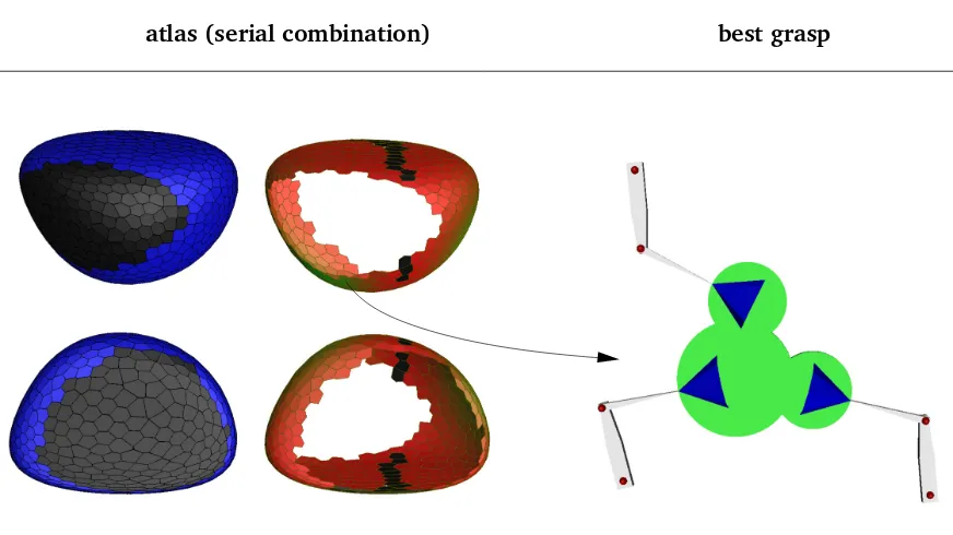
4.12 The best grasp of the SA hand under a serial combination of criteria . . . 66

5.1 Different hand actuations system . . . 71

5.2 Kinetostatic model of a grasp . . . 72

5.3 Representation of a spatial spring modeling a compliant contact . . . 76

5.4 Solutions obtained for a simple hand . . . 81

5.5 Solution obtained for the Schunk Anthropomorphic hand . . . 83

5.6 Executing a solution on THE First hand . . . 83

6.1 Mapping between a mechanical hand and a sensorized glove . . . 91

6.2 A human hand with a sensorized glove . . . 92

6.3 Schematic representation of the experimental setup . . . 92

6.4 Correlation of joints in the hand configuration space . . . 95

6.5 Configurations of the SA hand using two PMDs independently . . . 96

6.6 Configurations of the SA hand using combinations of two PMDs . . . 96

6.7 Total variance covered when using an increasing number of PMDs. . . . 97

6.8 The goal configuration used to define the point of interest . . . 99

6.9 The 4-dimensional submanifold that satisfies the orientation constraint . 100 6.10 Rotation matrixR1 used to define the orientation constraint . . . 100

7.1 A2-dimensional spaceXhmodelled with two PMDs . . . 105

7.2 Samples of the hand-arm system . . . 107

7.3 Roadmap under construction . . . 113

7.4 Qualitative comparison between the classical and proposed approach . . 115

7.5 Simulation and real execution of a solution path . . . 115

7.6 Hand-arm goal configurations for some of the benchmark tasks . . . 117

7.7 Solution paths of two benchmark tasks . . . 118

Tables

3.1 Representative hand designs adopted during the last decade . . . 26

3.2 Test cases and their computed solutions . . . 39

3.3 Parameters of the SA hand . . . 42

5.1 Notation used in the kinetostatic model of a grasp . . . 73

5.2 Kinematic and elastic parameters for the planar hand . . . 82

5.3 Kinematic and elastic parameters of THE First hand . . . 84

6.1 Correspondence between the glove sensors and the hand acuators . . . . 94

7.1 Parameters used in the approach path planner . . . 116

7.2 Quantitative comparison of the proposed and classical approaches . . . . 116

7.3 Comparison of the planner performance on several benchmark tasks . . 118

7.4 Computation time of the planner when considering and omitting the orientation constraint . . . 119

Part I

1

Introduction

The human hand, the most versatile end-effector provided by Nature, can perform such a variety of motions and subtle adjustments that mimicking its abilities mechanically has been qualified as the Holy Grail of robotic end-effectors [9]. This chapter outlines the main motivations underlying the pursuit of such abilities, delimits particular objectives and scope of this Ph.D. work, and summarizes the structure of the dissertation.

1.1 Motivation

Figure 1.1: Commercially available robotic hands by Shadow Robot Company [107] (left) and Schunk GmbH & Co. KG [106] (right).

1.1 Motivation 5

bottom). Driven by the potential benefits of such hands, progress towards building hands for practical applications is underway, and the first commercial hands, such as the Shadow [107] and Schunk [106] hands, have recently come to light, allowing to picture out an increasing number of applications in the future, in classical or emerging contexts like service robotics, telemedicine, space exploration, prosthetis, manipulation in hazardous environments, or human-robot interaction.

1.2 Objectives and scope

Several aspects have to be addressed before realizing the dream of a robotic hand with human-like capabilities, ranging from the consolidation of a proper mechatronic design, to the development of precise, lightweight sensors and actuators, to the efficient planning and control of the finger forces and motions required for interaction with the envrionment. The aim of this thesis is to provide suitable solutions to a main problem within the latter aspect, known as the grasp planning problem: Given a robotic system formed by a multifinger hand attached to an arm, and an object to be grasped, both in a known geometry and location in 3-space, determine how should the hand-arm system be moved without colliding with itself or with the environment, in order to firmly grasp the object in a suitable way, allowing to perform a specific manipulation task (Figure 3.1).

1.2 Objectives and scope 7

Figure 1.3: Grasp planning: Given a robotic hand-arm system and an object (left), determine how should the system be moved in order to grasp the object in a suitable way, avoiding collision with itself or with the environment (right).

end-effectors may adopt a variety of designs, with a range of kinematic topologies, link geometries, and actuation schemes, we will require our algorithms to be of sufficient generality to be able to apply them to any particular instance of such designs. This will entail adopting general numerical techniques for kinematic constraint solving in their implementation, since they are the only ones that have proved to be powerful enough to solve non-linear systems of equations of the kind that arise. Fourth, we will assume that accurate geometric models of the object, the hand-arm system, and the environment are available, so that the planning of motion paths can safely be made using them.

A divide-and-conquer strategy will be used to overcome the complexity of the grasp planning problem, breaking it up into the following subproblems:

1. The grasp synthesis problem: Determine a grasp configuration satisfying a num-ber of hand-object contact constraints, while guaranteeing the manipulability and restrainability of the object at the same time.

Figure 1.4: While the GraspIt! suite [20, 37, 64] is nicely suited to generate random grasps able to hold an object (left), it cannot produce specific grasps allowing a particular manipulation of the object (right). This PhD work aims at solving the grasp planning problem in the latter context.

A solution to the grasp planning problem will be obtained by devising modules able to solve the previous two subproblems. The grasp synthesis module provides a hand configuration in contact with the object, which can be fed to the approach path planning module to generate a goal configuration for the overall hand-arm system, using standard inverse kinematics techniques for the supporting arm. Once such a goal configuration is available, the latter module can start the search for a joint-space path connecting the current configuration of the system to the mentioned goal configuration.

1.3 Outlook at the dissertation

The dissertation is structured into four parts, which can be outlined as follows:

• Part Iprovides the motivation, objectives and scope of the work (Chapter 1), and encloses a short account on the state of the art on the two topics related to this thesis (Chapter 2).

1.4 Glossary 9

the computation of a configuration of the hand-object system that respects all assembly constraints imposed by the hand joints, and all hand-object contact constraints considered (Chapter 3). Next, a second algorithm is developed that, departing from the grasp configuration computed by the previous algorithm, is able to explore the manifold of hand configurations in contact with the object, to find those that are the maximally restrained and manipulable. The technique is general enough to cope with usual force-closure or manipulability metrics, com-binations of such metrics, or any other metric that might be defined (Chapter 4). Finally, the fact that both the joints and the hand-object contacts are actually non-rigid is taken into account, and a way to synthesize grasp configurations where such joints and contacts behave according to given compliance models is introduced (Chapter 5). The technique is general enough to tackle the kinematic and restrainability constraints at once, and only requires to be initialized with an estimation of the solution, which can be computed using the techniques developed in the preceding chapters.

• Part IIIpresents the solution given to the approach path planning problem. Firstly, a meaningful way to reduce the dimension of the hand configuration space is proposed. The approach draws inspiration from how the human hand moves in the free space to lessen the finger freedom by coordinating the joint movements, and biases the wrist orientation towards the goal by imposing relational position-ing constraints (Chapter 6). This reduction is later on exploited to develop an algorithm that solves the approach path planning problem in an adaptive way, adjusting the configuration space dimension where needed, according to the local obstacle complexity encountered at each step (Chapter 7).

• Part IV, finally, draws the main conclusions of the thesis, summarizes its contribu-tions, and enumerates points deserving further attention (Chapter 8).

1.4 Glossary

For the sake of clarity, we next define basic terminology used throughout the manuscript.

intended to provide an end-effector of similar versatility to that of the human hand. The number of fingers must be at least three to grant sufficient stability. The fingers must have at least two links acting as phalanges, articulated through lower-pair joints. The number of joints must be at least three per finger, with at least three actuators per finger. The joint distribution must allow the finger to produce abduction/adduction and flexion/extension motions.

Task-specific contact constraint: A contact constraint that must necessarily be ful-filled in order to manipulate the object in a specific way. Such constraints are assumed to be given, and take the form of general patch-patch contact constraints, so that a surface patch defined on the hand is enforced to be in contact with a corresponding patch defined on the object, with the normal vectors to the patches aligned. The hand patches can be defined anywhere on the finger or palm surfaces.

Configuration of the hand-object system: A description of the position and orienta-tion of all bodies involved in the hand and the object, respecting the joint assembly constraints of the hand only. In such a configuration, the hand may or may not be in contact with the object.

Grasp: A particular configuration of the hand-object system in which the hand is in contact with the object, but not necessarily satisfying any of the task-specific contact constraints assumed.

Kinematically-feasible grasp: A grasp that satisfies all of the imposed task-specific contact constraints.

1.4 Glossary 11

Manipulable grasp: A grasp that is able to perform controllable object motions along arbitrary directions of its pose space. Again, various metrics can be defined to assess the quality of a manipulable grasp.

Arm: A serial kinematic chain acting as a carrying device for a robotic hand. The arm must be able to move the hand throughout large portions of its pose space, that is, both in position and orientation. Six-revolute arms will be considered for concreteness, but the presented techniques can be applied to general serial arms.

2

Related Work

This chapter provides a short account of previous work related to the problems of grasp synthesis and approach path planning dealt with in this Thesis. Along the way, the reader is pointed to related sections of the manuscript where such techniques play an important role, or where an enhancement or alternative to them is given.

2.1 Grasp synthesis

Figure 2.1: Whereas a force-closed grasp relies on friction (left), a form-closed grasp relies on shape to restrain the object (right). [Images courtesy of the Human Grasping Database [31].]

foundations for finding them. From that point, the external wrench applied to the object was related to the forces applied at the contacts through the so-called grasp matrix, and qualitative tests were provided to determine whether a given set of wrenches restrained an object [102], which naturally led to quantitative tests [33, 89, 116]. By using these tests, numerous approaches have been developed for synthesizing contact points in 2D [22, 58, 70, 73] and 3D [10, 56, 77, 78, 87] objects.

2.1 Grasp synthesis 15

All of the works just mentioned provide useful insights into key aspects of grasp planning, but the resulting algorithms are of limited applicability in practice, because the hand configuration in contact with the object is either neglected, despite being fundamental to the force-closure concept adapted to grasping [5], or assumed to be given, but never synthesized in any case. Recently, a more comprehensive approach to the problem has been attempted, which emphasizes the computation of hand config-urations in contact with the object from the very beginning, in addition to searching for an optimal grasp [20]. The main difficulty in this case is that the set of hand configurations in contact with the object is a complex manifold, implicitly defined by a system of non-linear equations that expresses all joint-assembly and contact constraints involved in the hand-object system. To avoid this complexity, Ciocarlie and Allen [20] initially relax the contact constraints, resulting in a search space that coincides with the configuration space of the hand. Typically, this space is of a high dimension, but meaningful simplifications derived from the use of hand postural synergies [104] can be introduced to narrow the search to a subspace explorable in reasonable times, using simulated annealing. The hand configurations obtained, however, are not exactly in contact with the object and, thus, they must be evaluated with pre-grasp quality indices, which involves purely geometric features only. Unfortunately, a grasp qualified as good using these indices does not always result in a high-quality grasp once the contact with the object is finally enforced using local techniques, or by simply closing the fingers until contact is achieved. The final hand-object contacts, moreover, are not necessarily suitable for a specific task and, hence, the technique is nicely suited to generate random grasps able to hold an object, but not those grasps allowing a particular manipulation of the object.

neural network to learn the finger inverse kinematics, and on reinforcement learning to optimize the pose of the hand, and Rosell et al. [95], who propose an iterative method to compute joint displacements that maximally reduce the distance from the fingertips to the desired contact points. Such methods are usually fast and return solutions in many cases, but their convergence is not always guaranteed, even if a solution exists. Some of the methods, moreover, require a sufficiently-good initial estimation of the solution [11, 95], which might not always be available.

A way around such limitations will be worked out in Chapter 3, by proposing a new algorithm of guaranteed convergence; i.e., one that always provides a hand configura-tion satisfying the required contact constraints whenever one exists. This algorithm does not require an initial estimation of the solution and can, in fact, solve a superclass of the configuration problems dealt in [11, 38, 95], because all contact constraints considered in such works can be seen as particular cases of more general ones tractable herein.

Regardless of the adopted method to compute a grasp, it is worth noting that the grasp is usually not optimized in terms of any quality criterion, so that a final opti-mzation process is needed to obtain a suitable high-quality grasp. Implementing such a process is not trivial though, since trying to optimize the grasp in a generate-and-test fashion is computatinally too expensive, and local optimization methods like [75] are likely to get trapped into local optima because, except in simpler cases [57, 111], grasp quality indices present local extrema. A grasp optimization procedure that avoids such drawbacks will be proposed in Chapter 4, based on tracing a set of relevant grasps exhaustively using a higher-dimension continuation technique. A rigid-grasp model is assumed in such a procedure, but a way to take grasp compliance into account will be given in Chapter 5.

2.2 Approach path planning

2.2 Approach path planning 17

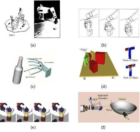
either very close to the obstacle region, or directly on its border. A main trend since the early attacks to the problem, thus, has been to simplify the problem in some way or another, either by using simpler hands or restricted actuation schemes, or by assuming favorable uncluttered environments. Nevertheless, the increase of computational power over the years, and the appearance of succesful probabilistic roadmap methods, has allowed to progressively drop some of these simplifications, gradually increasing the range of solvable problem instances (Figure 2.2).

One of the earliest works on the problem was that by Lozano-Perez et al. [61] on the Handey system, which involved a classical one-degree-of-freedom gripper mounted on a six-revolute arm, aimed at performing pick-and-place operations for assembly tasks. In this system, the planning of an approach path to the object was subdivided into two-stages. First, using a cell-decomposition method, a path involving gross motions of the arm was computed during a global stage in order to bring the gripper in close proximity to the object. Then, a simple path taking the system to the final grasp was generated during a local stage, using a potential field method. Although several simplifying assumptions were made in both stages —including planar-faced objects, motions involving only three joints, and a relatively uncluttered environment around the object— the Handey system was taking many aspects of the problem into con-sideration, and many subsequent works are still reminiscent of the two-stage strategy adopted. The work in [61] was extended by Pollard [76] later on, replacing the gripper by the more complex, three-fingered Salisbury hand. The planning of the path was done under similar assumptions, using cell-decomposition and potential field methods for the global and local stages, but more involved grasp synthesis methods were introduced to account for the increased complexity and reconfiguration capacity of the newer hand. The grasp configuration was synthesized by choosing proper contact points for the fingertips, together with a feasible pose for the wrist heuristically, and an attempt to connect this configuration to an intermediate configuration at a given distance from the object was then made using a straight-line path possibly deformed locally, so that the latter configuration could be easily reached by the global planner.

no planning of the approach path to the object, since the pre-grasp configuration is informed, and the closing of the fingers is deterministic. However, Morales et al. [67] extended this approach to account for more complex objects and hands, alleviating the need of informing manually the system with pre-grasp configurations. In their case, the pre-grasp configuration is automatically selected from a database of previously-computed pre-grasps, and the final approach path to the object, taken as well from the database, follows a straight-line pattern similar to the one used by Pollard [76], but allowing the rotation of the wrist about the path if necessary. In simulation, the planner iteratively translates the hand along the path, and possibly rotates it, checking along the way whether the resulting hand configuration can properly reach the object by closing the fingers.

Aiming to deal with more cluttered environments, Berenson et al. [2] propose to rank all possible approach paths a priori before trying them, using a score function that quantifies the promise of the path to yield a high-quality, collision-free grasp in the end. The paths considered are identical to those tried by Morales et al. [67] but, once one of them is found to be valid, the system is able to plan a motion from the start configuration of the hand-arm system, to the pre-grasp configuration determined, using bi-directional Rapidly-exploring Random Trees (RRTs). The hand configuration is kept constant during such planning in order to grow the trees in six-dimensional joint spaces only. Berenson and Srinivasa [3] present a refinement of the technique in which all degrees of freedom of the hand are allowed to move in a coordinated way during the exploration of the final approach path, adding one additional degree of freedom that increases the chances of succeeding along the path.

A slight twist to these approaches has been recently introduced by Vahrenkamp et al. [118], in an attempt to integrate the grasp synthesis and approach path planning phases to the largest possible extent. In their work, a global planner iteratively grows an RRT from the initial configuration of the hand-arm system, selecting one of its nodes randomly from time to time for exploration towards the object. This exploration, which is similar to that in previous approaches, consists in trying a linear path until a threshold position around the object is reached, then closing the fingers until contact is established, and finally evaluating the grasp using typical grasp quality metrics.

2.2 Approach path planning 19

(a)

(c)

(e)

(b)

(d)

(f)

final grasp configuration will be suitable to a particular manipulation task involving the object. In most grasp planning systems the hand is simply closed from a pre-grasp configuration, so that it is difficult to predict in which precise object regions will the fingers finally land. Second, the overall grasp planner is usually a combination of global and local planners whose domain of application is heuristically defined with rule-of-thumb conditions that seem artificial to the problem. Third, the hand-arm system is usually set to move under simplified motion paths only, which restricts the range of possible movements, and hence the ability to find proper solutions in complex situations with cluttered environments.

Part II

3

Finding Grasp Configurations

This chapter presents a method to compute a kinematically-feasible grasp, i.e., one that satisfies a given collection of hand-object contact constraints. In contrast to previous algorithms given for the same purpose, the one presented here allows specifying such contact constraints between free-form surface patches on the hand and object surfaces, and always returns a solution whenever one exists. The method is based on formulating the problem as a system of polynomial equations, and then exploiting the special form of the equations to isolate the solutions, using a numerical technique based on linear relaxations. Although explained for anthropomorphic hands, the approach is general, in the sense that it can be applied to any grasping mechanism with lower-pair joints. The approach can also accommodate as many hand-object contacts as required, involving any of the hand links, including the palm.

h1

h2

h3

h4

o1

o2 o3

o4

Figure 3.1: A typical grasp for a scalpel can be specified by requiring the contact of regions h1, . . . , h4 of the hand, with regionso1, . . . , o4 on the object (left). The problem is to determine how should the hand be configured relative to the object, in order to bring the hand regions into contact with their corresponding object regions (right).

3.1 The hand-object system

3.1.1

Structure of an anthropomorphic hand

Although each anthropomorphic hand follows a particular design, all hands are in general made up of a palm and several fingers, one of them acting as the thumb. Usually, all fingers are aligned with each other and with the palm, except the thumb, which is mounted asymmetrically so that it can push against the other fingers. Each finger is composed of several phalanges, usually articulated through revolute (R) or universal (U) joints, whose freedom may be actuated, underactuated, or coupled to those of other joints. Mechanical limitations usually exist, that constrain these joints to take values within prescribed ranges.

3.1 The hand-object system 25

U

R

R

Figure 3.2: The URR structure of a finger. remaining axes, which are usually

parallel, are responsible for flex-ion/extension movements of the finger. The thumb structure is more diverse and controversial [36, 119]. Designs are found where the thumb adopts the same structure as that of the remaining fingers, which facilitates the construction of the hand, like in the SA hand, for instance. Other designs either decrease or increase the mobility of the thumb, by removing or adding joints with respect to the basic URR design. In all cases, however, the tip of the thumb is allowed to face all other fingertips, so as to be able to grasp and manipulate objects under stable prehensions.

A summary of representative hand designs adopted during the last decade is pro-vided in Table 3.1. In order to reduce the number of actuators, note that many hands have coupled degrees of freedom. The coupling of two joints A and B is indicated as ⁀

#Actuated Finger designs

Hand d.o.f. Little Ring Middle Index Thumb

DIST hand[1998] 16 - URR

Robonaut hand[1999] 12 RR⁀RR⁀ URR⁀ UR⁀

LMS hand[2001] 16 - URR

Ultralight Anthropom. hand[2001] 10 RRR⁀ U⁀RR⁀

GIFU II hand[2002] 16 URR⁀ URR

Shadow Robot hand[2003] 18 RURR⁀ URR⁀ UUR

DLR II hand[2004] 13 - URR⁀ RURR⁀

UBH 3 hand[2004] 20 URR

MA-I hand[2005] 16 - URR

SA hand[2012] 13 - URR⁀ RURR⁀

Twendy-One hand[2009] 13 - URR⁀ RUR

Table 3.1: Representative hand designs adopted during the last decade.

3.1.2

Contact constraint specification

The contact constraints are assumed to be given as a collection of pairs (hc, oc), for

c= 1, . . . , b contacts, where hc and oc are two-dimensional regions on the hand and

object surfaces, respectively. The constraint(hc, oc)is meant to require the contact ofhc

and oc at some point, with the normals to hc and oc aligned at such point, to avoid the

interpenetration of the regions (Figure 3.3).

By convention,hc and oc are assumed to be given as polynomial patches. That is, it

is assumed that a polynomial function of the form

p=p(u, v), (3.1)

is given for each region, providing the parametric coordinates p = (px, py, pz) of a

pointP in the region, in terms of some scalar parametersuandv, bound to lie within the interval[0,1]. To properly align the normals ofhc andoc, the parameterizationp(u, v)is

supposed to be non-degenerate, in the sense that, ifpuandpv are the partial derivatives

of p(u, v)with respect touandv, then the normal vector to the patch, defined as

3.1 The hand-object system 27

never vanishes for(u, v)∈[0,1]×[0,1].

For ease of explanation, p(u, v) will adopt the form of a standard Bézier patch of some given degreeM ×N,

p(u, v) =

M

X

i=0

N

X

j=0

bi,j·Bi,M(u)·Bj,N(v), (3.3)

where bi,j denote the Bézier control points of the patch, and Bi,j(x) = j_i

xi_(1−x)j−i

is theith Bernstein polynomial of degreej. Note that any polynomial paramaterization

p(u, v)can be converted into such form, by using an appropriate change of basis [30].

Lk Ln

Hc Oc

ˆ mc

ˆ nc

oc

hc

Figure 3.3: Elements intervening in a contact constraint (hc, oc). The constraint is

satisfied when points Oc ∈ oc and Hc ∈ hc coincide, with the normals on such points

3.2 Kinematic equations

A kinematically-feasible grasp can be formulated as a number of constraints that the poses of the hand and object links must fulfill. This section formulates such constraints mathematically, following the methodology proposed by Porta et al. [80]. Once gath-ered together, the constraints form a system of polynomial equations characterizing all possible solutions of the problem. The special structure of this system will be beneficial to solve the problem numerically, as it will be shown in Section 3.3.

3.2.1

Link constraints

It will be convenient to label the hand and object links asL0, L1, . . . , Ln, whereL0 is the palm link, L1, . . . , Ln−1 are the various phalange links, and Ln is the object link. The

joints of the hand will also be labelled for reference, asJ1, . . . , Jm.

Each link Ll, l = 0, . . . , n, will be furnished with a local reference frameFl, and we

will let the reference frame of the palm link,F0, to act as the absolute frame. Moreover, each frame will have an associated vector basis, and we will write vFl to refer to the coordinates of vectorv, written in the basis ofFl. Vectors with no superscript will either

be expressed in the basis of the absolute frame, or in no particular frame, depending on the context.

With the previous notation, a configuration of the hand-object system will be an assignment of a pose (rl,Rl)to each link Ll, l = 1, . . . , n, where rl ∈R3 is the position

of the origin of Fl with respect toF0, andRl ∈SE(3) is a3×3 rotation matrix giving

the orientation of Fl relative to F0. The elements of the rotation matrices are not independent, because ifRl has the form(ˆcl,ˆdl,ˆel), then it must be

kˆclk2 = 1, (3.4)

kdˆlk2 = 1, (3.5)

ˆcl·dˆl = 0, (3.6)

ˆcl×dˆl = ˆel, (3.7)

for l = 1, . . . , n, in order for Rl to represent a valid rotation. Note that the joints, the

3.2 Kinematic equations 29

3.2.2

Joint assembly constraints

Since most hand designs only resort to revolute or universal joints (Table 3.1), we focus on formulating the constraints imposed by such joints, but other joint types would be formulated in a similar way [80].

In terms of spatial constraints, the assembly of two links Lj and Lk, through a

revolute joint Ji, is equivalent to imposing the coincidence of two points, Pi and Qi,

and the alignment of two unit vectors, ˆui and ˆvi, respectively fixed to Lj and Lk

(Figure 3.4a). These two points and vectors are chosen on the axis of the joint, and they

Lj Lj Lj Lj Lk Lk Lk Lk (a) (b) (c) (d) ˆ ui,ˆvi

ˆ ui

ˆ vi

Pi, Qi Pi, Qi ˆ ui ˆ vi Pi Pi Qi Qi ˆ

ui _vˆi

90o

coalesce into a single point and vector when the two links get assembled (Figure 3.4b). The coincidence and alignment conditions can be written, respectively, as

rj +Rjp

Fj

i =rk+RkqFik, (3.8)

Rjuˆ

Fj

i =RkvˆFik, (3.9)

where pFj

i and q

Fk

i refer to the position vectors of Pi and Qi in frames Fj and Fk,

respectively. The valid poses of the two links, hence, are those that fulfill Eqs. (3.8) and (3.9) simultaneously.

Similarly, ifJi is a universal joint, the valid poses ofLj andLk are those that fulfill

rj +Rjp

Fj

i =rk+RkqFik, (3.10)

Rjuˆ

Fj

i ·RkˆviFk = 0, (3.11)

where Eqs. (3.10) and (3.11) impose the coincidence of two pointsPi andQi, and the

orthogonality of two unit vectors ˆui andvˆi, respectively fixed onLj andLk. The points

are located on the center of the universal joint, on Fj and Fk. The vectors are aligned

with the axes of the joint on such frames (Figures 3.4c and 3.4d). Since vectors pFj

i ,

qFk

i , uˆ

Fj

i , and ˆv

Fk

i are known a priori, the only unknowns in Eqs. (3.8)-(3.11) are the

poses of the two links (rj,Rj)and(rk,Rk).

3.2.3

Joint limit constraints

For a revolute jointJiincident to linksLj andLk, the relative angle betweenLj andLk,

denotedφi, is the angle between two unit vectorsˆai andˆbi orthogonal to the axis ofJi,

fixed in Lj and Lk, respectively. Usually, due to the existence of mechanical limits, φi

can only take values within a prescribed interval which, using a proper location for ˆai

and bˆi, can always be written in the form [−αi, αi], withαi ∈[0, π]. In our formulation,

these limits can be taken into account by constraining the cosine of φi. For this, we

define a new variable ci = cos(φi), and observe that the constraint φi ∈ [−αi, αi] is

equivalent to the constraint ci ∈[cosαi,1]. Then we note that

3.2 Kinematic equations 31

where

ˆ

ai =Rj ˆa

Fj

i , (3.13)

ˆ

bi =RkbˆFik. (3.14)

Thus, to constrainφito the range[−αi, αi]it is only necessary to add Eqs. (3.12)-(3.14)

to the system to be solved, taking into account thatci can only take values in the range

[cosαi,1]. Joint limits for a universal joint can be imposed in a similar way.

3.2.4

Contact constraints

Let us suppose that in the required grasp some hand linkLk is required to be in contact

with the object link Ln, where the contact has to be established between given regions

hc and oc defined onLk and Ln, respectively (Figure 3.3). LetHc ∈ hc and Oc ∈ oc be

two points on such regions, with position vectors hFk

c and oFcn relative to Fk and Fn,

respectively, and let mˆc and ˆnc denote unit normal vectors to the link surface at such

points. Then, the poses of Lk and Ln that bring the two regions in contact through Hc

andOc are those that fulfill

rk+RkhFck =rn+RnoFcn, (3.15)

RkmˆFck =−RnnˆFcn, (3.16)

where Eq. (3.15) imposes the coincidence ofHc and Oc, and Eq. (3.16) establishes the

alignment ofmˆc and ˆnc.

All vectors and matrices in Eq. (3.15) are unknowns. However, sinceHc and Oc are

bound to lie onhc andoc, the additional constraints

hFk

c =h

Fk

c (uc, vc), (3.17)

oFn

c =o

Fn

c (sc, tc), (3.18)

must be taken into account to properly formulate the contact, where hFk

c (uc, vc) and

oFn

c (sc, tc)are parametric descriptions of regionshcandoc, given in the form of Eq. (3.3).

Note that the Bézier control points of the patches hFk

c (uc, vc) and ocFn(sc, tc) must be

Analogously, the unit vectorsmˆFk

c and ˆnFcn in Eq. (3.16) must also be related to the

patch parameters. This relationship can be established by taking into account that, for a parametric patch p(u, v)of the form of Eq. (3.3), the normal vectorn(u, v)defined by Eq. (3.2) can be written as

n(u, v) = 2M−1

X

i=0 2N−1

X

j=0

b′_i,j·Bi,2M−1(u)·Bj,2N−1(v), (3.19)

so that it can be thought of as a new Bézier patch, but now of degree(2M−1)×(2N−1). Explicit formulas for computing the control pointsb′

i,j in this expression, in terms of the

control points bi,j of p(u, v), are given by Yamaguchi [123]. Thus, mˆcFk and nˆFcn can

be related to the patch parameters by defining two unnormalized vectors mFk

c andnFcn,

and their norms µc and νc, placed in correspondence with mˆcFk and nˆFcn through the

constraints

µ2_c =kmFk

c k

2_{, (3.20)}

ν_c2 =knFn

c k2, (3.21)

mFk

c =µcmˆFck, (3.22)

nFn

c =νcnˆFcn, (3.23)

and setting the additional constraints

mFk

c =m

Fk

c (uc, vc), (3.24)

nFn

c =n

Fn

c (sc, tc), (3.25)

whose right-hand sides follow the form of Eq. (3.19).

3.2.5

Final system of equations

3.3 Numerical Solution 33

• The pose variables(rl,Rl)corresponding to linksLl,l = 1, . . . , n.

• The variablesˆai,bˆi, andcicorresponding to the joint limit constraints on all joints

Ji,i= 1, . . . , m.

• The contact point coordinateshFk

c and oFcn, associated normal vectors mcFk, nFcn,

ˆ mFk

c ,nˆFcn, vector normsµc andνc, and parametersuc,vc,sc, andtc, corresponding

to all contact constraints(hc, oc),c= 1, . . . , b.

It is worth mentioning that the rlvariables of this system can actually be eliminated

through a process explained in detail in [80]. The elimination is based on the fact that, for a loop of links pairwise constrained by joint or contact constraints, Eqs. (3.8), (3.10), and (3.15) occurring along the loop can be substituted by an equivalent “loop-closure” equation which is their sum, which does not contain any of therlvariables. This process

simplifies the system, and can always be invoked if desired, but the numerical method that follows is equally applicable to both the original and the simplified system.

3.3 Numerical Solution

Let ne and nv be, respectively, the number equations and variables of the final system

described in Section 3.2.5. This system can be compactly written as

Φ(q) = 0, (3.26)

where q = (q1, . . . , qnv) refers to a vector encompassing all of its variables, andΦ is a

polynomial function from Rnv _toRne _{describing its equations. We now wish to develop} a method to find a pointqsatysfying Eq. 3.26, whenever one exists.

In a third approach, branch-and-prune methods use approximate bounds of the so-lution set to rule out portions of the search space that contain no soso-lution, reducing the initial domain as needed until a fine-enough approximation of the solution is ob-tained [17, 27, 63, 80, 85].

While algebraic-geometric and continuation methods are general, they have a num-ber of limitations in practice. On the one hand, algebraic-geometric methods usually explode in complexity, may introduce extraneous roots, and can only be applied to relatively simple systems of equations. On the other hand, continuation methods should be implemented in multi-precision arithmetic to avoid numerical instabilities, leading to important memory requirements and, like elimination methods, they must compute all possible roots, even the complex ones, which are physically meaningless in our case, thus slowing the process substantially on systems with a small fraction of real roots. Branch-and-prune methods are also general, and present a number of advantages that make them preferable in our case: (1) Contrarily to many elimination methods, they do not require intuition-guided symbolic reductions, (2) they directly isolate the real roots, (3) they can be made numerically robust without resorting to extra-precision airthmetic, and (4) some of them can tackle under- and over-constrained problems without needing modifications. These are the main reasons that motivate the approach we adopt next, which belongs to this latter category. The approach, which is based on the one proposed in [80], entails expanding the equations to a standard form (Subsection 3.3.1) and then using a branch-and-prune method exploiting this form to isolate the solutions (Subsections 3.3.2 and 3.3.3).

3.3.1

Equation expansion

We distinguish two groups of equations in the final system Φ(q) = 0. A first group encompassing Eqs. (3.17), (3.18), (3.24), and (3.25), whose polynomials follow the Bézier form of Eqs. (3.3) and (3.19), and a second group encompassing the remaining equations, whose polynomials only contain monomials of the form qi,q2i and qiqj. Note

that all equations of the second group can be easily converted into linear form by introducing the changes of variables

pi =qi2 (3.27)

3.3 Numerical Solution 35

for all q2

i and qiqj monomials occuring in them. After such changes, we obtain a new

system of the form

Λ(x) = 0 Ψ(x) = 0

)

, (3.29)

where x is an nx-dimensional vector encompassing all of the original qi variables, and

the newly-introduced pi and bk ones. Here, Λ(x) = 0 represents a collection of linear

equations in x, and Ψ(x) = 0 represents a collection of equations, each of which can only adopt one of these three forms:

xk =x2i, (3.30)

xk =xixj, (3.31)

xk =f(xi, xj). (3.32)

While the first two forms correspond to the changes of variables in Eqs. (3.27) and (3.28), the latter form corresponds to the scalar components of Eqs. (3.17), (3.18), (3.24), and (3.25), so thatf(xi, xj)refers to a Bernstein-form polynomial of degrees di and dj

inxi and xj, respectively.

3.3.2

Equation solving

It can be seen that, under the used formulation, each variable xi of x can only take

values within a prescribed interval [80], so that the Cartesian product of all such intervals defines an initial nx-dimensional box B ⊂ Rnx which bounds all solutions of

Eqs. (3.29). The algorithm to isolate such solutions recursively applies two operations onB: box shrinkingand box splitting.

As it turns out, this algorithm explores a binary tree of boxes, whose internal nodes correspond to boxes that have been split at some time, and whose leaves are either solution or empty boxes. By properly implementing the bookkeeping of boxes awaiting to be processed, this tree can be explored either in depth- or breadth-first order, the choice of order depending on whether one wishes to isolate just one solution, or the entire solution set.

Note that the algorithm is complete, in the sense that the solution boxes it returns include all solution points of Eqs. (3.29). Thus, the algorithm will always succeed in isolating a solution, whenever one exists, provided that a small-enough value of the σ parameter is used. Detailed properties of the algorithm, together with examples of its output, are given by Porta et al. [79, 80].

3.3.3

Box shrinking

We next see how a given sub-boxBc ⊆ Bcan be reduced, discarding portions of the box

that contain no solution. Observe that the solutions of Eqs. (3.29) lying within Bc ⊆ B

must lie on the linear variety defined by Λ(x) = 0. Thus, in principle, we might shrink Bc to the smallest possible box bounding this variety inside Bc. The lower and upper

limits of the shrunk box along dimensionxi, i= 1, . . . , nx, would respectively be found

by solving the two linear programs

LP1:Minimize xi, subject to: Λ(x) = 0,x∈ Bc,

LP2:Maximizexi, subject to: Λ(x) = 0,x∈ Bc.

The sub-box Bc may be further reduced, however, because the solutions must also

satisfy the equations Ψ(x) = 0. These equations can be taken into account by noting that for each equation it is possible to define a convex polytope that bounds the equation solutions within Bc. Thus, to better delimit the solutions of the system,Bc can be safely

reduced to the smallest possible box enclosing the intersection of Λ(x) = 0 and the polytopes of all equations in Ψ(x) = 0. This reduction can be implemented by repre-senting the individual polytopes with linear inequalities, and adding such inequalities to the constraint set of the linear programsLP1andLP2. We next see how such polytopes can be derived, for each one of Eqs. (3.30)-(3.32). The notation [li, ui]will refer to the

3.3 Numerical Solution 37 (a) (b) (c) A1 A2 A3 B1 B2 B3 B4 xk xk xk xj xj xi xi xi ui ui ui li li li uj uj lj lj C01 C02 C10 C11 C12

C20 C21

C22

Figure 3.5: Polytope bounds within Bc. (a) The points on xk = x2i are bound by the

triangleA1A2A3. (b) The points on xk=xixj are bound by the tetrahedronB1B2B3B4. (c) The points on xk =f(xi, xk)are bound by the convex hull of the pointsCpq. In this

example,f(xi, xk)is a Bernstein-form polynomial of degree two inxi andxj, so that the

control pointsCpq form a grid of size3×3.

To derive a polytope for xk =x2i, note that the portion of the parabolaxk =x2i lying

withinBc is bounded by the triangleA1A2A3 in thexi-xkplane, whereA1andA2are the points where the parabola intercepts the lines xi = li and xi = ui, and A3 is the point where the tangent lines atA1 andA2 meet (Figure 3.5a). Thus, the polytope ofxk =x2i

To derive a polytope forxk =xixj, we realize that the portion of the surfacexk =xixj

included inBcis bound by a tetrahedronB1B2B3B4 in thexi-xj-xksubspace, whose

ver-ticesBi are obtained by lifting the four corners of the rectangle[li, ui]×[lj, uj]vertically

to the surface xk = xixj (Figure 3.5b). Thus, the polytope of xk = xixj is defined by

the tetrahedron B1B2B3B4, and can be represented by four inequalities, corresponding to the four faces of this tetrahedron. Finally, to derive a polytope for xk = f(xi, xj),

we resort to the subdivision and convex-hull properties of Bernstein polynomials [30]. Using the subdivision property, on the one hand, f(xi, xj)is written in the form

f(xi, xj) = di X p=0 dj X q=0

bp,q·Bp,di(xi)·Bq,dj(xj),

where the scalars bp,q are the so-called control points off(xi, xj) relative to the

inter-val [li, ui]×[lj, uj]. Using the convex-hull property, on the other hand, we know that

the surfacexk=f(xi, xj)must be contained inside the convex-hull of the 3D pointsCpq

with coordinates

cpq =

li+ p

di(ui−li), lj+ q

dj(uj−lj), bp,q

, (3.33)

forp= 0, . . . , di, andq= 0, . . . , dj (Figure 3.5c). This convex hull defines a polytope for

equation xk=f(xi, xj), which can be encoded as a set of inequalities by resorting to an

algorithm for convex-hull computations [1].

3.4 Test cases

The presented method has been implemented in C, extending the libraries of the CUIK suite [80]. This section illustrates the performance of the method under this implemen-tation, on various test cases where an object needs to be grasped in a particular way, in order to fulfill a given task.

3.4 Test cases 39

Number of contacts 2 (slightly constrained) 3 (moderately constrained) 4 (highly constrained)

SCALPELtasks Upholding Handling Incision

Task requirements It requires picking the scalpel up using the index finger and the thumb.

It requires handling the scalpel delicately using the middle finger, the thumb, and the palm.

It requires a pencil-like grasp using two fingers, the thumb, and the palm.

nv,ne,d 219,209,17 243,235,16 331,324,18

CPU time[s] 106 255 418

Computed solution

TEAPOTtasks Lid lifting Service Transportation

Task requirements The lid must be pulled up through its knob using the index finger and the thumb.

The hand is required to hold the teapot by its handle, plac-ing the thumb on top, while the index and middle fingers embrace it.

The palm contacts the bottom of the teapot, while the fingers enclose it so that it does not slide out.

nv,ne,d 219,209,17 288,278,19 312,305,17

CPU time[s] 114 262 375

Computed solution

GUITARtasks Tunning Playing Holding

Task requirements It requires the hand to grasp a given key using the index fin-ger and the thumb to tune the tension of the corresponding string.

The fingertips must be at specified strings and frets to perform a chord, while the thumb contacts the guitar neck.

It requires a whole-hand grasp on a specific region where the guitar can not be damaged while being transported.

nv,ne,d 219,209,17 307,298,19 331,324,18

CPU time[s] 68 229 664

Computed solution

of the fingertip area (the dark patches on the upper limbs in Figure 3.6b), the area of the contact regions on the object varies from experiment to experiment, from2% of the fingertip area on the teapot knob (“lid lifting” experiment), to 9000%of such area on the guitar neck (“playing” experiment).

We next explain how the equations of the hand can be set up, and later discuss the algorithm’s performance on the mentioned tests.

3.4.1

Equations for the Schunk Anthropomorphic hand

The Schunk Anthropomorphic hand is composed of four identical fingers that follow the anthropomorphic structure illustrated in Figure 3.2. Three of these fingers are directly mounted on the palm, and act as ring, middle, and index fingers. The fourth finger is mounted on an intermediate link articulated with the palm through a revolute joint, which allows this finger to act as a thumb (Figure 3.6). The hand has a total of fourteen links (one palm and thirteen phalanges) and thirteen joints (nine revolute joints and four universal joints).

To set up the equations, the links of the hand are labelled as L0, . . . , L13, as shown in Figure 3.6, and the joints as J1, . . . , J13, letting Ji be the joint between Li−1 and Li

(for clarity, joint labels are not shown in Figure 3.6). Twenty-six points and unit vectors are then defined, that provide the positions and orientations of all rotation axes of the hand relative to the involved links. The points correspond to the centers of the universal joints and to the midpoints of the revolute joints. The vectors correspond to unit vectors aligned with the rotation axes of the joints. These points and vectors are displayed in Figure 3.6 and their coordinates are given in Table 3.3, in milimeters. All reference frames Fl are located with their origin in Ql, so that qlFl = (0,0,0), for l = 0, . . . ,13.

The orientations of such frames can be deduced easily from the coordinates provided in Table 3.3. Taking into account these definitions, Eqs. (3.4)-(3.11) can readily be written for all links and joints involved.

To write down the equations of Section 3.2.3, the mechanical limits of the SA hand must be considered. Regarding the universal joints, the rotations about their uˆi and

ˆ

vi axes are limited to the ranges [−15o,15o] and [−4o,75o], respectively. Regarding the

revolute joints, all of them can only rotate in the range [4o_,75o_{], except for the revolute}

joint at the base of the thumb, which is restricted to the range [0o_,90o_{]. The reference}

3.4 Test cases 41 (a) _(b) palm ring middle index thumb L0 L1 L2 L3 L4 L5 L6 L7 L8 L9 L10 L11 L12 L13 ˆ u1 ˆ v1 P1 Q1 ˆ u2 ˆ v2 P2 Q2 ˆ u3 ˆ v3 P3 Q3 ˆ u4 ˆ v4 P4 Q4 ˆ u5 ˆ v5 P5 Q5 ˆ u6 ˆ v6 P6 Q6 ˆ u7 ˆ v7 P7 Q7 ˆ u8 ˆ v8 P8 Q8 ˆ u9 ˆ v9 P9 Q9 ˆ u10 ˆ v10

P10 _Q

10 ˆ u11 ˆ v11 P11 Q11 ˆ u12 ˆ v12 P12 Q12 ˆ u13 ˆ v13 P13 Q13 Q0 U U R R R R R

Figure 3.6: Geometric parameters (a) and reference configuration (b) of the Schunk Anthropomorphic Hand. The various joint types are indicated in (b).

Finally, it must be taken into account that not all joints of the SA hand are indepen-dently actuated. The two distal joints of each finger are coupled, so that when one of such joints is actuated, a rotation of the same angle about the other is produced. In the adopted formulation, the coupling of two rotation angles is simply imposed by equating the sine and cosine of such angles.

3.4.2

Computed solutions

Joint Ring Middle Index Thumb

type Par. Value Par. Value Par. Value Par. Value

R

pF2

3 (30,0,0) p

F4

6 (30,0,0) p

F7

9 (30,0,0) p

F12

13 (30,0,0)

ˆ uF2

3 (0,1,0) ˆu

F5

6 (0,1,0) uˆ

F8

9 (0,1,0) ˆu

F12

13 (0,1,0)

ˆ vF3

3 (0,1,0) ˆv

F6

6 (0,1,0) ˆv

F9

9 (0,1,0) ˆv

F13

13 (0,1,0)

R

pF1

2 (67.80,0,0) p

F4

5 (67.80,0,0) p

F7

8 (67.80,0,0) p

F11

12 (67.80,0,0)

ˆ uF1

2 (0,1,0) ˆu

F4

5 (0,1,0) uˆ

F7

8 (0,1,0) ˆu

F11

12 (0,1,0)

ˆ vF2

2 (0,1,0) ˆv

F5

5 (0,1,0) ˆv

F8

8 (0,1,0) ˆv

F12

12 (0,1,0)

U

pF0

1 (−4.30,−40.16,145.43) p

F0

4 (−4.30,0,145.43) p

F0

7 (−4.30,40.16,145.43) p

F10

11 (97,6,−87)

ˆ uF0

1 (1,0,0) ˆu

F0

4 (1,0,0) uˆ

F0

7 (1,0,0) ˆu

F10

11 (cos 55

o_{,0,sin 55}o₎

ˆ vF1

1 (0,1,0) ˆv

F4

4 (0,1,0) ˆv

F7

7 (0,1,0) ˆv

F11

11 (0,1,0)

R

pF0

10 (−3,27.10,0)

ˆ uF0

10 (0,0,−1)

ˆ vF10

10 (1,0,0) Table 3.3: Parameters of the Schunk Anthropomorphic hand.

do not intervene in any kinematic loop, and hence impose no loop-closure constraint on the overall system.

Table 3.2 provides the size of the equation system Eq. (3.26) to be solved in each case, in terms of the number of variables, nv, and equations, ne, it involves, and the

dimension of its solution space, d, predicted as the number of variables minus the number of non-redundant equations. Note in this regard that Eq. (3.9) introduces equations that are redundant in terms of predicting such dimension, because uˆi and

ˆ

vi are unit vectors, and it is sufficient to establish two out of the three components

of Eq. (3.9) to determine the alignment of Lk relative to Lj. The third component of

Eq. (3.9), however, is needed to remove a sign ambiguity in such alignment. Since a similar redundancy is introduced by Eq. (3.16), there will be as many redundant equations as the number of joints and contacts involved in the problem at hand.

3.5 Summary 43

DELL Poweredge computers, equipped with two Intel Quadcore Xeon E5310 processors and a 4Gb RAM each one, using a threshold ofσ= 0.1. Note that the cost of computing a solution increases with the number of contact constraints to be satisfied. This is because the size of the linear programs to be solved during box shrinking is proportional to the number of polytope inequalities introduced by such constraints, which increases the cost of each iteration of the algorithm (Subsection 3.3.3).

3.5 Summary

4

Optimizing Grasp Configurations

This chapter provides a method for optimizing the quality of a robotic grasp, subject to satisfying a number of hand-object contact constraints of the kind assumed in the preceding chapter. Due to the multi-modal nature of typical grasp quality measures, approaches that resort to local optimization methods are likely to get trapped into local extrema on such problem. An additional difficulty of the problem is the fact that the set of feasible grasps is a highly-dimensional manifold, implicitly defined by a system of non-linear equations. The proposed procedure finds a way around these issues by focusing the exploration on a relevant subset of grasps of lower dimension, and tracing this subset exhaustively using a higher-dimensional continuation technique. Using this technique, a detailed atlas of the subset is obtained, on which the highest-quality grasp according to any desired criterion, or a combination of criteria, can be readily identified.

Figure 4.1: Two grasps of a can for drink service. While both grasps are force-closed and manipulable, the grasp on the left is preferable. The fingers are almost fully extended in the grasp on the right, limiting the possibility to move the can in one direction.

4.1 Kinematically-feasible grasps

Recall that, a kinematically-feasible grasp is a configuration of the hand-object system in which a number of regions of the hand hi, for i = 1, . . . , b, are in contact with

corresponding regions oi on the object. The regions and their pairings are pre-specified,

and the contact between hi and oi is assumed to be established with a point Hi ∈ hi

coinciding with another point Oi ∈ oi, keeping aligned the surface normals at such

points, mˆi and ˆni, to avoid local hand-object inter-penetrations. We further assume

that the hand joints are independently actuated or mechanically coupled, but do not consider the case of adaptive underactuated hands [9].

Independently of the particular formulation adopted, a grasp configuration can be represented by a vector x= (x⊤_h,x⊤_o,x⊤_c)⊤ _∈Rn _{of generalized coordinates, where x}

h and xo encompass the configuration variables of the hand and the object, respectively, and xc encompasses contact-related variables. Without loss of generality, we will as-sume that the absolute reference frame is attached to the palm of the hand, so that its pose variables do not intervene in x.

The variables inxare subject to a number of constraints. A first set of equations,

H(xh) = 0, (4.1)

4.1 Kinematically-feasible grasps 47

constraints imposed by the joints, usually revolute or universal, on the various bodies they connect, that is, the palm and the several finger phalanges. Note that Eq. (4.1) is not necessary if the xh coordinates are independent, as it happens for instance when choosing joint angles to represent a configuration [26]. In our case, however, we resort to the dependent coordinates defined in the previous chapter because they are equations of a simple structure, which has proved to be beneficial in the context of grasp synthesis (Chapter 3), and for the application of continuation techniques [121]. In particular, this formulation encodes the six degrees of freedom of a body with twelve variables, providing the position vector and the rotation matrix of a reference frame attached to the body. Therefore, in addition to the joint assembly equations, Eq. (4.1) includes constraints to enforce the 12-tuple of each body to be a member of SE(3). Similarly, the spatial pose of the object is encoded by twelve variables, so that a second set of equations,

L(xo) =0, (4.2)

constrains xo ∈ R12 to define a member of SE(3). Finally, a third set of equations formulates the contact constraints between the hand and the object. As in Chapter 3, we assume that each contact regionhi on the hand is specified as a parametrized patch,

i.e., as a smooth function of the form

hi =hi(ui, vi,xh), (4.3)

providing the absolute coordinates of a pointhi = (xi, yi, zi)in the patch, in terms of two

bounded scalar parameters, ui and vi, and of the hand configuration xh. Analogously, the normal to any point in this patch is assumed to be given as a function

ˆ

mi =mi(ui, vi,xh). (4.4)

In general, Eqs. (4.3) and (4.4) define two-dimensional regions described, for example, by Bézier patches [30], but they can be replaced by single-parameter curves or fixed points, if desired. The points and normals for the contact patches on the object can be defined in a similar way

oi =oi(si, ti,xo), (4.5)

ˆ