[1] A.V. Aho, J.E. Hopcroft, and J.D. Ullman.The design analysis of computer algorithms. Addison-Wesley, 1976.
[2] A.V. Aho, J.E. Hopcroft, and J.D. Ullman. Data structures and algorithms. Addison-Wesley, 1983.
[3] J.A. Bangham, P. Chardaire, C.J. Pye, and P.D. Ling. Multiscale non-linear decompo-sition: the sieve decomposition theorem. IEEE Transactions on Pattern Analysis and Machine Intelligence, 18(5):529–539, May 1996.
[4] J.A. Bangham, P.D. Ling, and R. Harvey. Scale-scape from nonlinear filters. IEEE Transactions on Pattern Analysis and Machine Intelligence, 18(5):520–528, May 1996.
[5] J.A. Bangham and J. Ruiz. The segmentation of images via Scale-Space Trees. In Proceedings of British Machine Vision Conference, pages 33–43, Southhampton (UK), September 1998.
[6] J.A. Bangham, J. Ruiz, and R. Harwey. Robust morphological Scale-Space Trees. In Proceedings of the Noblesse Workshop on Non-Linear Model Based Image Analysis, pages 133–139, Glasgow (UK), July 1998.
[7] J. Benois-Pineau, F. Morier, D. Barba, and H. Sanson. Hierarchical segmentation of video sequences for content manipulation and adaptive coding. EURASIP Signal Processing, 66(2):181–201, April 1998.
[8] G.D. Borshukov, G. Bozdagi, Y. Altunbasak, and A.M. Tekalp. Motion segmentation by multistage affine classification. IEEE Transactions on Image Processing, 6(11):1591– 1594, November 1997.
[9] E.J. Breen and R. Jones. An attribute-based approach to mathematical morphology. In Mathematical Morphology and Its Applications to Image Processing, pages 41–48, Atlanta (GA), USA, May 1996. Kluwer Academic Publishers.
[13] R. Chiariglione. MPEG and Multimedia Communications. IEEE Transactions on Cir-cuits and Systems for Video Technology, 7(1):5–18, February 1997.
[14] G.C.H. Chuang and C.C. Kuo. Wavelet descriptor of planar curves: theory and appli-cations. IEEE Transactions on Image Processing, 5(1):56–70, January 1996.
[15] J. Cichosz and F. Meyer. Morphological image segmentation. InProceedings of Work-shop of Image Analysis for Multimedia Interactive Services, pages 161–166, Louvain-La-Neuve, Belgium, June 1997.
[16] J. Crespo, J. Serra, and R.W. Schafer. Theoretical aspects of morphological filters by reconstruction. Signal Processing, 2(47):201–225, 1995.
[17] J. Crespo, R.W. Shafer, J. Serra, C. Gratin, and F. Meyer. A flat zone approach: a general low-level region merging segmentation method. EURASIP Signal Processing, 62(1):37–60, October 1997.
[18] J.L. Dugelay and H. Sanson. Differential methods for the identification of 2D and 3D motion models in image sequences. EURASIP Image Communication, 7:105–127, 1995.
[19] P.E. Eren, Y. Altunbasak, and A.M. Tekalp. Region-based affine motion segmentation using color information. In IEEE International Conference on Acoustics, Speech and Signal Processing (ICASSP), volume 4, pages 3005–3008, Munich, Germany, April 1997.
[20] M. Flickner, H. Sawhney, W. Niblack, J. Ashley, Q. Huan, B. Dom, M. Gorkani, J. Hafner, D. Lee, D. Petkovic, D. Steele, and P. Yanker. Query by image and video content: the QBIC system. IEEE Computer, 28(9):23–32, September 1995.
[21] L. Garrido, P. Salembier, and D. Garc´ıa. Extensive operators in partition lattices for image sequence analysis. EURASIP Signal Processing, 66(2):157–180, April 1998.
[22] C. Gomila. Mise en correspondance de partitions en vue du suivi d’objets. PhD thesis, Ecole Nationale Sup´erieure des Mines de Paris, September 2001.
[23] C. Gomila and F. Meyer. Levelings in vector spaces. InIEEE International Conference on Image Processing (ICIP), volume 2, pages 929–933, Kobe, Japan, October 1999.
[25] I. Grinias and G. Tziritas. Motion segmentation and tracking using a seeded region growing method. In European Signal Processing Conference (EUSIPCO), pages 921– 924, Rhodes, Greece, September 1998.
[26] R.M. Haralick and L.G. Shapiro. Image segmentation techniques. Computer Vision, Graphics, and Image Processing, 1(29):100–132, January 1985.
[27] H.J.A.M. Heijmans. Theoretical aspects of gray-level morphology. IEEE Transactions on Pattern Analysis and Machine Intelligence, 13(6):568–592, June 1991.
[28] S.L Horowitz and T. Pavlidis. Picture segmentation by directed split and merge proce-dure. In Proceedings 2sn International Joint Conference on Pattern Recognition, pages 424–433, 1974.
[29] D. Knuth. The art of computer programming, volume III (Sorting and Searching). Addison-Wesley, 1973.
[30] D. Le Gall. MPEG: a video compression standard for multimedia applications. Com-munications of the ACM, 34:47–58, April 1991.
[31] B. Marcotegui. Segmentation algorithm by multicriteria region merging. In Mathemati-cal Morphology and Its Applications to Image Processing, pages 313–320, Atlanta (GA), USA, May 1996. Kluwer Academic Publishers.
[32] B. Marcotegui. Segmentation de sequences d’images en vue du codage. PhD thesis, Ecole Nationale Sup´erieure de Mines de Paris, April 1996.
[33] F. Meyer. Minimum spanning forest for morphological segmentation. InMathematical Morphology and its Applications to Image Processing, ISMM’94, pages 77–84. Kluwer Academic Publisher, 1994.
[34] F. Meyer. The dynamics of minima and contours. In Mathematical Morphology and Its Applications to Image Processing, pages 329–336, Atlanta (GA), USA, May 1996. Kluwer Academic Publishers.
[35] F. Meyer. From connected operators to levelings. InMathematical Morphology and its Applications to Image and Signal Processing, pages 191–198, Amsterdam (The Neder-lands), June 1998.
[36] F. Meyer. The Levelings. In Mathematical Morphology and its Applications to Image and Signal Processing, pages 199–206, Amsterdam (The Nederlands), June 1998.
[40] F. Mokhatarian, S. Abbasi, and J. Kittler. Efficient curvature-based shape represen-tation for similarity retrieval. In European Signal Processing Conference (EUSIPCO), pages 597–600, Rhodes, Greece, September 1998.
[41] F. Mokhatarian and A.K. Mackworth. A theory of multiscale, curvature-based shape representation for planar curves. IEEE Transactions on Pattern Analysis and Machine Intelligence, 14(8):789–805, August 1992.
[42] P. Monasse. Morphological representation of digital images and application to registra-tion. PhD thesis, Universit´e Paris IX-Dauphine, France, June 2000.
[43] P. Monasse and F. Guichard. Fast computation of a contrast-invariant image represen-tation. IEEE Transactions on Image Processing, 9(5):860–872, May 2000.
[44] K. Moravec, R. Harvey, J.A. Bangham, and M. Fisher. Using an image tree to assist stereo matching. InInternational Conference on Image Processing (ICIP), Kobe, Japan, October 1999.
[45] F. Morier, J. Benois-Pineau, D. Barba, and H. Sanson. Robust segmentation of mov-ing image sequences. In IEEE Internation Conference on Image Processing (ICIP), volume 1, pages 719–722, Santa Barbara (CA), USA, October 1997.
[46] O.J. Morris, M. de J. Lee, and A.G. Constantinides. Graph theory for image analysis: an approach based on the shortest spanning tree. IEE Proceedings, 133(2):146–152, April 1986.
[47] MPEG. MPEG-7 visual part of eXperimentation Model Version 4.0. Technical Report ISO/IEC JTC1/SC29/WG11/N3068, MPEG, Maui, USA, December 1999.
[48] W. Niblack, X. Zhu, J.L. Hafner, T. Breuel, D. Poncele´on, D. Petkovic, M. Flickner, E. Upfal, S.I. Nin, S. Sull, B. Dom, B.-L. Yeo, S. Srinivasan, D. Zivkovic, and M. Penner. Updates of the QBIC system. In SPIE Storage and Retrieval for Image and Video Databases VI, pages 150–173, San Jose (CA), USA, January 1998.
[50] M. Ortega, Y. Rui, K. Chakrabarti, and A. Warshavsky. Supporting ranked boolean similarity queries in MARS. IEEE Transactions on Knowledge and Data Engineering, 10(6):905–925, December 1998.
[51] N.R. Pal and S.K. Pal. A review on image segmentation techniques.Pattern Recognition, pages 1277–1294, 1993.
[52] M. Pard`as, P. Salembier, F. Marqu´es, and R. Morros. Partition tree for a segmentation-based video coding system. InIEEE International Conference on Acoustics, Speech and Signal Processing (ICASSP’96), volume IV, pages 1983–1986, Atlanta (GA), USA, May 1996.
[53] S. Peleg and H. Rom. Motion based segmentation. In 10th International Conference on Pattern Recognition, June 1990.
[54] F.K. Potjer. Region adjacency graphs and connected morhological operators. In Math-ematical Morphology and Its Applications to Image Processing, pages 111–118, Atlanta (GA), USA, May 1996. Kluwer Academic Publishers.
[55] W.H. Press, S.A. Teukolsky, W.T. Vetterling, and B.P. Flannery. Numerical Recipes in C: the art of scientific computing. Cambridge University Press, 2nd edition, 1992.
[56] H. Radha, R. Leonardi, and M. Vetterli. A multiresolution approach to binary tree representations of images. InIEEE International Conference on Acoustics, Speech and Signal Processing (ICASSP), pages 2653–2656, May 1991.
[57] H. Radha, M. Vetterli, and R. Leonardi. Image compression using Binary Space Par-titioning Trees. IEEE Transactions on Image Processing, 5(12):1610–1624, December 1996.
[58] K. Ramchandran and M. Vetterli. Best wavelet packet bases in a rate-distortion sense. IEEE Transactions on Image Processing, 2:160–175, April 1993.
[59] E. Reusens. Joint optimization of representation model and frame segmentation for generic video compression. EURASIP Signal Processing, 46:105–117, September 1995.
[60] Y. Rui, T.S. Huang, and S.-F. Chang. Image retrieval: current techniques, promising di-rections and open issues. Journal of Visual Communication and Image Representation, 10:39–62, March 1999.
for interactive content-based image retrieval. IEEE Transactions on Circuits and Video Technology, 8(5):644–655, September 1998.
[64] J. Ruiz Hidalgo. The representation of images using Scale Ttrees. Master’s thesis, School of Information Systems, University of East Anglia, Norwich (UK), October 1999.
[65] E. Saber and A.M. Tekalp. Region-based shape mathing for automatic image annotation and query-by-example. Journal of Visual Communation and Image Representation, 8(1):3–20, March 1997.
[66] P. Salembier. Morphological multiscale representation for image coding. EURASIP Signal Processing, 46:359–386, September 1994.
[67] P. Salembier and L. Garrido. Binary Partition Tree as an efficient representation for filtering, segmentation and information retrieval. InInternational Conference on Image Processing (ICIP), Chicago (IL), USA, October 1998.
[68] P. Salembier and L. Garrido. Binary Partition Tree as an efficient representation for image processing, segmentation and information retrieval. IEEE Transactions on Image Processing, 9(4):561–576, April 2000.
[69] P. Salembier and L. Garrido. Connected operators based on region-tree pruning. In Mathematical Morphology and its Applications to Image and Signal Processing, Palo Alto (CA), USA, June 2000.
[70] P. Salembier, L. Garrido, and D. Garc´ıa. Auto-dual connected operators based on iterative merging algorithms. InMathematical Morphology and Its Applications to Image Processing (ISMM), Amsterdam, The Netherlands, June 1998.
[71] P. Salembier, J. Llach, and L. Garrido. Visual segment tree creation for MPEG-7 description schemes. In International Conference on Multimedia and Expo, New York City (NY), USA, July 2000.
[73] P. Salembier, A. Oliveras, and L. Garrido. Motion connected operators for image se-quences. InEuropean Signal Processing Conference (EUSIPCO), volume II, pages 1083– 1086, Trieste, Italy, September 1996.
[74] P. Salembier, A. Oliveras, and L. Garrido. Anti-extensive connected operators for image and sequence processing. IEEE Transactions on Image Processing, 7(4):555–570, April 1998.
[75] P. Salembier and H. Sanson. Robust motion estimation using connected operators. In IEEE International Conference on Image Processing (ICIP), volume 1, pages 77–80, Santa Barbara (CA), USA, October 1997.
[76] P. Salembier and J. Serra. Flat zones filtering, connected operators and filters by reconstruction. IEEE Transactions on Image Processing, 7:1153–1160, August 1995.
[77] P. Salembier, L. Torres, F. Meyer, and C. Gu. Region-based video coding using math-ematical morphology. Proceedings of the IEEE, 83(6):843–856, June 1995.
[78] H. Sanson. Toward a robust parametric identification of motion on region of arbi-trary shape by non-linear optimization. In IEEE International Conference on Image Processing (ICIP), volume 1, pages 203–206, October 1995.
[79] J. Serra. Image Analysis and Mathematical Morphology. Academic Press, 1982.
[80] J. Serra. Image Analysis and Mathematical Morphology, volume II: Theoretical Ad-vances. Academic Press, 1988.
[81] J. Serra and P. Salembier. Connected operators and pyramids. In Proceedings of the SPIE, Image algebra and morphological image processing IV, volume 2030, pages 63–76, San Diego (CA), USA, July 1993.
[82] E. Shusterman and M. Feder. Image compression via improved quadtree decomposition algorithms. IEEE Transactions on Image Processing, 3(2):207–215, March 1994.
[83] T. Sikora. The MPEG-7 visual standard for content description – and overview. IEEE Transactions on Circuits and Systems for Video Technology, 11(6):696–702, June 2001.
[84] P. De Smet and D. De Vleeschauwer. Motion-based segmentation using a thresholded merging strategy on watershed segments. In IEEE International Conference on Image Processing (ICIP), volume 2, pages 490–493, Santa Barbara (CA), USA, October 1997.
processing, pages 193–200. Kluwer Academic, Dordrecht 1994.
[88] G.J. Sullivan and R.L. Baker. Efficient quadtree coding of images and video. IEEE Transactions on Image Processing, 3(3):327–331, May 1994.
[89] M.J. Swain and D.H. Ballard. Color indexing. International Journal of Computer Vision, 7(1):11–32, January 1991.
[90] L. Torres, D. Garc´ıa, and A. Mates. A robust motion estimation and segmentation approach to represent moving images with layers. InIEEE International Conference on Acoustics, Speech and Signal Processing (ICASSP), pages 2981–2984, Munich, Germany, April 1997.
[91] C. Vachier and F. Meyer. Extinction value: a new measure of persistence. InWorkshop on Nonlinear Signal and Image Processing (NSIP), pages 254–257, Halkidiki (Greece), June 1995.
[92] P.J. van Otterloo. A Contour-Oriented Approach to Shape Analysis. Prentice-Hall, 1991.
[93] L. Vincent. Grayscale area openings and closings, their efficient implementation and applications. In J. Serra and P. Salembier, editors, Mathematical Morphology and its Applications to Image Processing, pages 22–27, Barcelona, Spain, May 1993. UPC.
[94] L. Vincent. Morphological grayscale reconstruction in image analysis: applications and efficient algorithms. IEEE Transactions on Image Processing, 2:176–201, April 1993.
[95] L. Vincent and P. Soille. Watersheds in digital spaces: and efficient algorithm based on immersion simulations. IEEE Transactions on Pattern Analysis and Machine Intelli-gence, 12(39):1845–1855, December 1991.
[96] A.J. Viterbi and J.K. Omura. Principles of Digital Communications and Coding. New York McGraw-Hill, 1979.
[97] T. Vlachos and A.G. Constantinides. Graph-theoretical approach to colour picture segmentation and contour classification. IEE Proceedings, 130(1):36–45, February 1993.
[99] N. Wirth. Algorithms & data structures. Prentice-Hall, 1986.
[100] X. Yaowu, E. Saber, and A.M Tekalp. Object formation by learning in visual databases using hierarchical content description. In International Conference on Image Procesing (ICIP), Kobe (Japan), October 1999.
7.1
Contribution
Our objective in this thesis has been the discussion of region based processing of images and video sequences using hierarchical representations. Tree based structures have been chosen in front of graph-bases structures for the representation since the former are inherently hierar-chical and allow implementing efficient and complex techniques on it due to its fixed structure. The processing of these hierarchical structures has been based on pruning techniques, that is, techniques that remove several subtrees of the structure based on an analysis algorithm applied on the nodes of the tree structure. Moreover, the processing algorithms developed in this thesis have been restricted to a framework in which the input and the output of the processing are pixel based representations. Let us now briefly recall the main contributions of this thesis.
Two representations have been developed in our work: the Max-Tree, and the Binary Partition Tree. The former was created to address the efficient implementation of anti-extensive connected operators, ranging from classical ones (for instance, area filter) to new ones (such as the motion filter). The latter was developed initially to overcome some of the drawbacks imposed by the Max-Tree, but has demonstrated to be a structure useful for a rather large range of applications.
The general processing scheme in which our algorithms are enclosed is divided in two stages: in the first stage, the tree representation is constructed using the image or video sequence, whereas in the second step, the tree is processed and analyzed to decide how the tree has to be pruned.
used. The tree construction is, from our experience, the most computationally expensive task. Efficient algorithms based on the intensive use of hierarchical queues have been developed in order to enable fast construction of the tree.
Pruning techniques applied on the Max-Tree lead to anti-extensive operators, whereas self-dual operators are obtained on the Binary Partition Tree if the tree is created in a self-dual manner. In this work, pruning techniques have been targeted on filtering (connected operators), segmentation and content based image retrieval techniques. In the case of filtering and segmentation, the pruning strategy is based on performing an analysis of the nodes of the tree by measuring a specific criterion on each of the associated regions. Examples of available criteria discussed in this work are based on area, contrast ormotion. Other criteria, such as themarker & propagationbased orrate-distortionbased segmentation, have also been studied. The decision on the elimination or preservation is usually taken on each node by means of a simple threshold. A solution to the non-increasingness of some criteria based on an optimization algorithm has been presented and discussed. Furthermore, as discussed in this work, the analysis and decision steps are very efficient in terms of time and memory consumption. As a result, segmentation and filtering processing techniques, based on tree representations, may be used in an intensive manner.
The Binary Partition Tree has also been used for content based image retrieval. In fact, this tree structure offers a way to represent the image at different levels of resolution. As a result, the description can be done at different scales of resolution. The description has been done using only low level descriptors, namely color and geometry descriptors. Single and multiple region retrieval has been developed. From our experimental results, the quality and relevance of the retrieved results depend on whether a good segmentation has been obtained, which is one of the main difficulties in image analysis. However, as pointed out in the future research directions, multiple region query may be used to overcome this problem.
7.2
Future research
Within the differents parts discussed in this thesis the following research work may be devised:
Creation
Processing
• Filtering and segmentation: in this work the analysis algorithm is mainly based on the assessment of a criterion independently on each node and the use of a threshold to decide which nodes have to be removed or preserved. New methods based on the analysis of several nodes at a time for processing may be thus devised.
New types of filters using a combination of time and geometry descriptors may be devised. For instance, one may think of a filter that removes from a sequence all small regions whose global life span is less than a fixed threshold on the number of frames. These type of filtering may be interesting for content based coding applications.
• Content based image retrieval: the results of the content based retrieval engine may be enhanced by adding more descriptors to describe each region. Similarity based on fuzzy sets, as discussed in Sec. 6.6.7, may also improve the retrieval results.
Up to now, the hierarchy of the tree has not been really exploited to code in its nodes the region descriptors in an efficient manner. Efficient coding of descriptors is obtained if descriptors can be computed in a recursive manner (see Sec.6.4). The recursivity has been exploited to code the color histogram in an efficient manner. But, how does shape or texture behave under the union of two regions ? In other words, given the shape or texture descriptor of two neighboring regions, is it possible to compute or, at least approximate, the corresponding descriptor of the union of both regions ?
Multiple region search may overcome some of the problems posed of the tree creation through segmentation. In fact, the Binary Partition Tree is created by means of a segmentation algorithm and thus it is difficult to ensure that complex regions are rep-resented as a single region in the tree. In this case single region query would not work properly since the latter method needs to have the objects of interest to be represented as nodes in the tree. Future search work may study how to use multiple region search to be able to search for a fixed single object whose region of support has been divided in several nodes during the tree construction: the user may only define the whole region of support to search for and it would be the task of the search engine to decompose properly the query into subregions to perform the search.
in order to ensure that relevant objects are represented as nodes in the tree (object formation by learning [100]). A second topic of interest in relevance feedback is to study the possibility of using some of the relevant objects marked by the user as query to improve the results, in addition of properly updating the weights.
• Non-pruning operations: this work has focused on pruning operations. Further research work may focus on operations on nodes which do not lead to pruning operations. For instance, in [71] a method to restructure the tree in order to get a representation that reflects more clearly the image structure is presented.
6.1
Objectives
In the recent years, the size of digital image collections has increased rapidly. Everyday, giga-bytes of images and sequences are generated. This information it has to be organized so as to allow efficient browsing, searching and retrieval. In the last years, increasing interest has been paid to the study of image retrieval. For that purpose, two different strategies have been used to retrieve data: one based onmanual annotationsand one based onvisual features[60]. Even many advances have been made in the field text based retrieval, there exist major difficulties, especially when the size of the image collection is large. One difficulty is the vast amount of labor required to manually annotate images and a second difficulty, the subjectivity of human perception. The perception subjectivity and annotation impreciseness may cause unrecoverable mismatches in the later retrieval process [60]. Thus, the manual annotation strategy has become with the emergence of large image collections an acute problem.
To overcome these difficulties, Content Based Image Retrieval (CBIR) was proposed. Instead of manually annotating each image by text based keywords, images are indexed ac-cording to their own visual content, such as color, texture, etc. Many techniques in this research direction have been developed, and many systems, both research and commercial, have been built. Since 1997, one of the activities of the MPEG group is to unify the repre-sentation of multimedia content by proposing a standard to describe any type of multimedia document. The standard, known as MPEG-7 (Multimedia Content Description Interface), has challenging objectives given the broad spectrum of requirements and targeted multimedia applications, and the broad number of audiovisual features of importance in such context.
Many image retrieval systems, both commercial and research, have been built. Let us review a few representative systems. We focus only on the visual part of the system:
• QBIC [20,48], standing for Query By Image Content, was the first commercial content based image retrieval system. Developed at the IBM Almaden research center, QBIC supports queries based on example images, user constructed sketches and drawings, etc. Extracted descriptors on either images or objects are the color histogram and the Tamura texture representation. For the shape descriptor, the area, circularity, eccentricity, major axis orientation and a set of moments invariants are extracted.
• Virage [60] is a content based image search engine developed at Virage Inc. Similar to QBIC, Virage supports visual queries based on color, color layout, texture and object boundary information. Virage goes one step further than QBIC by supporting arbi-trary combinations of the previous four descriptors. The users can adjust manually the weights associated to the descriptors according to their needs.
• VisualSEEk [86,85] is a visual descriptor search engine developed at Columbia Univer-sity. The visual descriptors used in this system are color set [60] and wavelet transform based texture descriptor. To speed up the retrieval process, efficient indexing algorithms have been developed. VisualSEEk supports queries based on both visual descriptors and spatial relationships. This enables the user to submit a “sunset” query as a red-orange color region on top and a blue or green region at the bottom as its “sketch”.
• MARS [61, 50, 60] (Multimedia Analysis and Retrieval System) is developed at the University of Illinois at Urbana-Champaign. The main focus of MARS is not on finding a single “best” descriptor representation for each feature, but rather on how to organize various visual descriptors into a meaningful retrieval architecture which can dynami-cally adapt to different applications and users. MARS proposes a relevance feedback architecture for the retrieval process in order to adapt the query results to the users need.
From the above review, we can see that many advances have been made in the field of content based image retrieval. However, a long way has still to be covered before image retrieval can be of practical use.
hierarchical structure of the representation to enable retrieval at different levels of resolution. The efficient indexing of the data in the database is, however, out of the scope of this work.
The work described in this chapter has not been published up to date.
6.2
Supported Queries
Two types of queries are discussed in this chapter,
• Single region query (Sec. 6.5): the query is characterized by the fact that its associated region of support is one connected component. Our objective in this case is to search in the database for the target regions that visually match best the query. That is, we want to find regions whose descriptors are similar to those of the query.
• Multiple region query (Sec. 6.6): the query is made up of several (not necessarily dis-connected) regions. Our objective is to search in the database for a set of regions that match best the query. In other words, we want to look for a set of regions whose asso-ciated descriptors match those of the query, and at the same time these regions should have a spatial relationship similar to the query.
The features the search engine uses for similarity based retrieval can be combined in a flexible manner. In our work, similarity is obtained by means of a distance based on a weighted sum of several feature dissimilarities. The users need can be adapted by setting properly the values of the weights. In Sec.6.7 a method for automatically computing such weights is presented. Thus, the user is removed from the burden of manually setting such weights.
6.3
Tree processing strategy
Fig.6.1shows the scheme used in this chapter for content based region retrieval.
descriptor Region
descriptor Region
Database engine Search
BPT creation
Database construction
Query construction Query results
Figure 6.1: Content based image retrieval processing strategy.
is a simple text based file that lists all filenames associated to the files of Binary Partition Trees that should be included in the database. This rather simple strategy has been adopted due to the fact that our purpose in this chapter is to show that the hierarchical partition tree enables content based image retrieval. Efficient indexing techniques allowing faster searching should be envisaged in future works.
The user defines via a graphical user interface thequery object to search for (made up of the mask and pixel values). The query object together with the weights associated to the each of the descriptors used for the similarity assessment makes up the query.
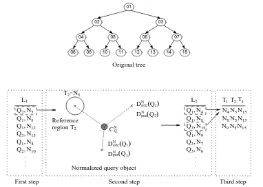
The associated region descriptors are then obtained from the query object. The search engine interacts with the database in order to find visually similar objects with respect to the query. In other words, the analysis algorithm associated to the search engine should select, among the set of nodes of the trees that are stored in the database, those whose contents are similar to those of the query. This search procedure can be seen as a tree pruning strategy. The pruning consists in removing the subtree associated to the selected nodes of the tree. There are several ways of presenting the result of the pruning to the users. One possible solution may be based on marking on the original image the region of support associated to the subtrees that have been pruned. As a result, the user is then able to see the regions that are visually similar to the query. In this work, an approach based on reconstructing only each pruned subtree on pixel based representation has been taken. In the case of single region query each resulting image contains one connected component, thus the tree processing algorithm prunes only one subtree from a tree (single region pruning). On the other hand, in the case of multiple region each resulting image should be composed of several connected components, thus multiple region pruning is performed on the trees of the database. Fig. 6.2
Multiple region pruning Single region pruning
6.4
Region Descriptors
Our purpose is to visually describe the regions that compose the nodes of the tree. Region descriptors are used for that purpose. In our work, two types of descriptors are attached to each region: color descriptors, which deal with the region content, andgeometry descriptors, which deal with parameters such as position, size, rotation and shape of the region. We will make use of the notation Ddesc(R) to reference the descriptor “desc” of regionR.
Moreover, we may take advantage of the hierarchical structure by attaching simple de-scriptors at each of the nodes. A node may be described by using its associated dede-scriptors giving us thus an approximate description of the region we are dealing with. However, if the descriptors attached to the descendants of the subtree of a node are used, a more precise description of the region can be obtained. This property may be used to code the description of the tree in an efficient way.
6.4.1 Color
Color is one of the most widely used visual features in image retrieval. It is independent of image size and orientation [60].
One of the simplest region color descriptor one may attach to the nodes of the tree is a constant color model, for instance the mean color value in the HSV or YUV space. As discussed previously, this color descriptor attached to a node may seem insufficient to represent its texture or even its visual appearance in a correct way. But by taking advantage of the hierarchical tree structure the region can be described at different scales of resolution. A region can be described using only the color descriptor attached to the associated node giving us thus a poor approximation of the inner content of the associated region. The maximum level of detail is reached when a node is described using the leaf nodes of the associated subtree. Observe that there is a relationship between the color model for a node and its children. For instance, if the model used to represent the color is the mean value of each color component, the model for a certain node can be computed simply by averaging the models of its children.
In image retrieval, the color histogram descriptor is the most commonly used color de-scriptor [60]. Statistically, it denotes the joint probability of the intensities of the three color channels. Color histograms are a way to represent the distributions of colors in images where each histogram bin represents a color in a suitable color space (RGB, HLS, YUV). The se-lected color space has to be discretized and the number of times each discrete color appears has to be counted. In our work, the YUV space is used, and the color histogram Dhisto(R) is
of bins of the color histogram isNBY U V =NBY ×NBU×NBV. In this work, we have taken
NBY =NBU =NBV = 16.
Since histograms are interpreted as a probability density function the following condition has to be satisfiedm: PNBY U V−1
k=0 Dhisto(R)[k] = 1 where Dhisto(R)[k] represents the k’th bin
of the color histogram of regionR.
6.4.2 Geometry
Geometry descriptors involve position, size, rotation and shape features. Descriptors of po-sition, size and rotation are easily extracted using the Hotelling transform, also known as Principal Component Analysis [24]. The Hotelling transformation analyzes the statistical properties of a population of vectors.
Consider the population of vectors p = (px, py), where px, py are the coordinates of the
pixels that belong to a region R. The mean vector is defined as mp = (mpx, mpy) = E{p}, and the covariance matrix of the population of vectors asCp =E{(p−mp)T(p−mp)}, where
(.)T stands for vector transposition
Cp =E
(px−mpx)(px−mpx) (px−mpx)(py−mpy) (px−mpx)(py−mpy) (py−mpy)(py−mpy)
!
Since Cp is real and symmetric, finding the two orthonormal eigenvalues is always possible.
Let ei and λi, i = 1,2 be the eigenvectors and corresponding eigenvalues of Cp. The next
step is to construct the matrixA, whose rows are formed by the eigenvectors of Cp, ordered
so that the first row ofA is the eigenvector corresponding to the largest eigenvalue. A is a transformation matrix that maps the population of vectors p into vectors denoted by q by the transformationq =A(p−mp). The population of vectorsq corresponds to the rotation
and position invariant representation of the regionR. Moreover, the covariance matrix of the population of vectorsq,Cq, is [24]:
Cq =
λ1 0
0 λ2
!
where λ1 = E{(qx−mqx)2} = E{qx2} (since mqx = 0) and λ2 = E{(qy −mqy)2} = E{qy2}
(sincemqy = 0).
Within this framework, mp corresponds to the position descriptor, Dpos(R) = mp. The
R1
R2
R’1
d12
R’2
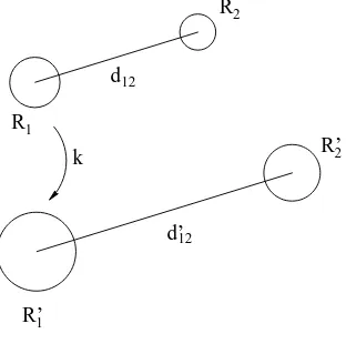
[image:21.595.210.366.119.274.2]d’12 k
Figure 6.3: Example of scaling a set of regions by a factor ofk.
that generates the matrix which corresponds to the rotation descriptor,Drot(R) =α. The size
descriptor is Dsize(R) =√λ1+λ2. This is equivalent to compute the mean squared energy
of the population of vectors of q, since,λ1 andλ2 are, respectively, the standard deviation of
the population p in the direction of its principal axis and its normal.
The previous descriptors are extracted from zero, first and second order moments. These can be extracted easily from the pixel based representation of the associated region of support. An efficient strategy based on the outer boundary contour is presented in [92]. In a continuous signal framework, the approach is based on transforming the double integral of the moment definition into a closed circular integral using Green’s theorem. The strategy is then translated to the discrete framework. Note however, that the values of the moments obtained with the pixel based coincide with the values obtained with the corresponding contour based approach if the region in the pixel based representation has no holes.
Moreover,Dsize(R) has an interesting property, namelyDsize(R′1) =kDsize(R1) if region
R′1 is a scaled version of R1 by a factor of k in bothx and y axis (that is, R′1 has the same
outer shape than R1 but its associated areas satisfy AR′
1 =k
2A
R1, where AR′1 and AR1 are
the size in pixels of regions R1 and R2 respectively). This property will be used for scaling
appropriately the query in the case of multiple region query. Fig. 6.3shows an example. The figure depicts to regions, R1 and R2, separated by a distance of d12. If region R1 is scaled
by a factor of k (AR′
1 = k
2A
R1), then, in order to maintain the proportions and distances
between regions properly, d12and R2 have to be scaled by a factor ofk.
Shape
perception of human visual system and offers good generalization; it is robust to non-rigid motion; it is robust to partial occlusion of the shape and it is compact.
The Curvature Scale Space (CSS) descriptor is obtained from the maxima of the CSS image. TheCSS imageis a multi-scale organization of the inflection points of a closed planar curve as it is smoothed. Let us now describe how the CSS image is obtained.
Let Γ be a closed planar curve, and let u be the normalized arc length parameter on Γ:
Γ(u) ={(x(u), y(u))|u∈[0,1]}
If Γ is convolved with a 1-D Gaussian kernel function of width σ, the resulting curve, Γσ,
will be smoother than Γ. Asσ increases, Γσ becomes smoother. Whenσ becomes sufficiently
high, Γσ will be a convex curve.
For each filtered curve Γσ, the associated curvatureτ(u) is computed according to
κσ(u) =
x′
σ(u)y′′σ(u)−x′′σ(u)yσ′(u)
x′
σ(u)2+yσ′(u)2
3/2
wherex′σ(u) (resp.yσ′(u)) denotes the first derivative of thexcomponent (resp.y) of Γσ, and
similarlyx′′
σ(u) (resp.yσ′′(u)) denotes its second derivative.
The zero crossings of the curvature function κσ(u), κσ(u) = 0, are then extracted for
each Γσ. The CSS image is created plotting the zero crossings in the plane (u, σ). That is,
a point is marked at the position (u0, σ0) if κσ0(u0) = 0. The horizontal axis in this image
corresponds to the locationu at which the zero crossing has been found, and the vertical axis corresponds is associated to theσ of the filter applied to the curve.
In the case of a discrete closed curve with samples γ[j] = {(x[j], y[j])|j∈[1, N]}, the curvature is a discrete signal κ[j]. First derivative of xσ[j] can be approximated as x′σ[j] =
xσ[j+ 1]−xσ[j−1] and second derivative as x′′σ[j] =x′σ[j+ 1]−x′σ[j−1]. Similar formulas
are used foryσ′[j] and y′′σ[j].
In Fig. 6.4an example of CSS descriptor computation is shown. The external contour of the original image shown on top is extracted using a contour tracking algorithm. The contour is then resampled toNsamples= 256 points. Linear interpolation is used to find values of the
Original image
After 0 iterations After 40 iterations After 120 iterations
[image:23.595.98.473.104.313.2]After 250 iterations After 600 iterations After 1200 iterations
Figure 6.4: Example of CSS descriptor computation. On top, the original image is shown. On bottom, smoothed versions of the original contour are depicted. The associated zero crossings are indicated with a cross on the curve.
the low-pass filter, the number of zero crossings decreases until the curve becomes convex, in which no zero crossings exists.
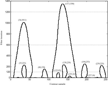
The associated CSS image is constructed from the set of zero crossings, see Fig. 6.5, indicating the evolution of the zero crossings of the curve as it is smoothed. The horizontal axis is associated to the position indexjof the curve, whereas the vertical axis is associated to the number of iterations of the low-pass filter applied to the curve. For instance, in Fig. 6.4
there are 14 zero crossings for the 120th iteration, 4 zero crossings for the 600th iteration and 2 zero crossings for the 1200th filter iteration. These zero crossing are correspondingly plotted in Fig. 6.5.
The CSS descriptor is extracted from the CSS peaks of the CSS image. Only the most significant peaks are detected. The x-coordinate of a maximum indicates the location where a pair of curvature zero crossings merge, and the y-coordinate of a maximum indicates the number of iterations needed until this merge actually happens. Fig. 6.5 indicates the CSS peaks that have been extracted. The extracted peaks are tabulated in Table 6.1(left). Only the peaks appearing after iteration 10 of the filtering are considered for posterior processing. The peaks are then normalized as follows [47]: the peaks position are first normalized to be in the interval [0,1] and then reordered so that the highest peak is in the position 0. For that purpose a circular rotation of the peaks positions have to be done. Note that this is equivalent to performing a rotation normalization of the curve descriptor. The peak height is transformed according to y′ = 6.0×y0.48
/Nsamples [47], where y is the height of the
0 50 100 150 200 250 0
200 400 600 800 1000
Contour sample
Filter iteration
(155,32)
(227,10) (35,233)
(88,159)
(139,239) (194,253)
(239,225)
(125,93) (34,1011)
120
Figure 6.5: Example of CSS image for the curve in Fig.6.4
Peak Position Peak Height
137 1350
34 1011
194 253
139 239
35 233
239 225
88 159
125 93
155 32
227 10
Norm. position Norm. height
0.000 0.745
0.597 0.648
0.226 0.333
0.011 0.324
0.601 0.320
0.398 0.315
0.808 0.267
0.953 0.206
0.070 0.123
0.351 0.070
[image:24.595.101.515.130.455.2]a) Extracted CSS peaks. b) CSS peaks after normalization.
All normalized peaks that are lower than 5% of the highest normalized peak are discarded. Note that by using this threshold, little peaks, usually due to noise in the curve, are removed from the descriptor. This makes the resulting descriptor more robust to noise. Table 6.1
(right) shows the normalized peaks that are used for the CSS descriptor. The CSS peaks are ordered according to the peak height.
The extracted CSS peaks do not depend of shape eccentricity. By using only the CSS peaks it is not possible to distinguish, for instance, between two convex shapes with different eccentricity (both have no CSS peaks). Thus, in addition to the CSS peaks, it seems necessary to use additional information to be able to differentiate between two shapes having the similar CSS peaks but different eccentricities. A global curvature vector is used for that purpose. The global curvature vector is made up of a floating point vector. The vector components represent the eccentricity and circularity of the original curve, respectively. The eccentricity of the curve can be computed directly from the PCA analysis previously described (eccentricity(R) = ∨(λ1, λ2)/∧(λ1, λ2)) whereas the circularity also is easy to extract (circularity(R) =∂R2/AR,
where AR is the area in pixels of regionR).
The CSS descriptor has been included in the MPEG-7 standard as one of the shape descriptor. Note that the descriptor is not able to distinguish regions with holes from regions without holes having the same external contour. The problem can be solved by representing each of the boundary of the holes using the CSS descriptor combined with its position relative to the over-whole region. Other solutions based on using a region based descriptor (such as Zernike moments [47]) can also be used.
6.5
Single region query
6.5.1 Query strategy
The user has to provide the search engine with the example of the query object (mask and pixel values) to search for. The search through the database is done by first computing the region descriptors for the region of support of the query (see Sec. 6.4). The search algorithm then looks for the set of regions in the tree database whose contents are similar to those of the query. For that purpose, the algorithm performs a sequential search through all the nodes of the trees in the database.
Let us denote with Q the query object and with T the target object against which the query is matched. Within this framework, T is a node of the tree of the database.
6.5.2 Region similarity
Color histogram
The color histogram is used to describe the color contents of a region. Let Dhisto(Q) and
Dhisto(T) represent, respectively, the color histogram of the query object Q and the target
object T. Color histograms define an equivalence function on the set of all possible colors, namely two colors are the same if they fall into the same bin. In [89] a matching strategy based on an L1 metric, the histogram intersection, is proposed. To take into account the
similarities between similar but not identical colors, in [20] an L2 metric is proposed. The
dissimilarity betweenDhisto(Q) and Dhisto(T) is assessed as aquadratic form
Shisto(Q, T) = (Dhisto(Q)−Dhisto(T))W(Dhisto(Q)−Dhisto(T))T
where W = [wij] is a matrix and wij denotes the similarity between bins i and j. These
weights are normalized so that 0≤wij ≤1, with wii= 1, where large wij (wij ≈1) denotes
high similarity between (color) bins i and j, and small wij (wij ≪ 1) denotes dissimilarity
between bins i and j. That is, each wij in the matrix W tries to capture the perceptual
similarity between the colors represented by binsiand j.
The following matrixW provides good results for our purpose: wij =exp
− 1 20dij
wheredij =
p
(Yi−Yj)2+ (Ui−Uj)2+ (Vi−Vj)2, andYi,Ui,Vi (resp. Yj,Uj,Vj) represent
the color components for the bini (resp. j). This matrix has been obtained experimentally by seeking for a color similarity matrix satisfying the conditions defined in the previous paragraph. Note that bell-shaped functions (such as the exponential) are well suited for our purposes. The function takes the following values: dij = 14 (resp. dij = 46),wij ≈0.5 (resp.
wij ≈0.1).
In order to reduce the amount of memory required to store the matrix in memory, sparse matrix storing [55] techniques are used. Moreover, only those weights wij greater than a
threshold are stored in memory.
Geometry descriptor
The dissimilarity of the size descriptor, Dsize(R), between the query Q and the target T is
assessed by evaluating
Ssize(Q, T) =
W
(Dsize(Q), Dsize(T))
V
(Dsize(Q), Dsize(T)) −
The position descriptor distance is obtained as follows:
Spos(Q, T) =
v u u t
Dx pos(Q)
Sizexf(Q) − Dx
pos(T)
Sizexf(T)
!2
+ D
y pos(Q)
Sizeyf(Q) −
Dposy (T)
Sizeyf(T)
!2
(6.2)
where Dx
pos(Q) andDposy (Q) (resp. Dxpos(T) andDypos(T)) are, respectively, the xand y
com-ponents of the position descriptor of the query (resp. target) region. Similarly, Sizexf(Q) and Sizeyf(Q) (resp. Sizexf(T) and Sizeyf(T)) represent the image width and height, respectively, of the original images that contain the query regionQ(resp. targetT) region. This approach has been taken in order to obtain a position dissimilarity assessment independent of the image size, however, this implies that the image size has to be attached at each tree included in the database.
Shape
The shape of every region of the tree in the database is represented by the normalized locations of the maxima of its associated CSS image together with a global and a prototype curvature vector (see Sec. 6.4.2).
Let us describe now the approach used to compare two sets of maxima. The present strategy is a slight modification of the approach presented in [39,47]. Assume that we want to match the CSS maxima of the query object Q, PQ, against the CSS maxima of a target
objectT,PT. The main idea behind the algorithm is to match each of the peaks of the query
Q against a peak of the targetT. A simple solution for this issue consists in finding, for each peak of the queryQ, a peak of the targetT that can be considered to be “near” to the former one in terms of, for instance, Euclidean distance.
Fig. 6.6 shows a rough idea of the approach used to perform the matching. On top of Fig. 6.6, the CSS of the query and the target are shown. Both CSS are assumed to be normalized according to Sec. 6.4. On the bottom-left corner we plot the CSS of the target over the one of the query. The peaks of the target are matched against the ones of the query according to Euclidean distance between the peaks if its circular distance between its peak positions is lower than, say 0.1. On the left of Table 6.3 the established matchings and associated cost (Euclidean distance) are indicated. For non-matched peaks the cost is defined to be the height of the non-matched peak. A CSS distance can be then computed by adding the contribution of the cost of each matching.
Query peaksPQ Target peaksPT
Table 6.2: Numerical values of the CSS peaks of the query and the target for the example of Fig.6.6.
PeakQ PeakT Cost PQ[1] PT[1] 0.08
PQ[2] PT[2] 0.14
PQ[3] PT[3] 0.07
PQ[4] – 0.10
PeakQ PeakT Cost PQ[1] PT[2] 0.07
PQ[2] PT[3] 0.31
PQ[3] – 0.20
PQ[4] – 0.10
– PT[1] 0.78
a) Matched peaks for first b) Matched peaks for second rotation normalization rotation normalization
Table 6.3: Matched peaks for the proposed rotations of Fig.6.6.
of the query (resp. target). Two sets of maxima matchings can be obtained. On bottom-left corner of Fig. 6.6, the CSS target has been rotated so that the peak position of PT[1] is 0,
whereas on the bottom-right corner of Fig. 6.6 the CSS has been rotated so that the peak position ofPT[2] is 0. The associated matchings are indicated in Table6.3. In conclusion, the
proposed matching algorithm takes into account several possible rotations in order to find a set of meaningful peak matching combinations.
Next the efficient implementation of the previous matching algorithm is discussed. Let NPQ (resp. NPT) denote the number of peaks associated to the CSS descriptor of the query
Q(resp. targetT) region, and PQ[i] with 1≤i≤NPQ (resp. PT[j] with 1≤j ≤NPT) the
i’th (resp. j’th) peak of the query (resp. target) region normalized as described in Sec.6.4.2. The matching algorithm is as follows:
1. Count the number NP80%Q of peaks of Q whose height is at least 80% of the highest peak of Q. Also, count the numberNP80%T of peaks of T whose height is at least 80% of the highest peak of T. A list L1 is created: each item k of the list L1, L1[k], will
store a different matching combination between the peaks of Q and T. The list is initialized by storing in each item a different pair (PQ[m], PT[n]) of CSS peaks, where
1 0.78 0.19 0.5 0.63 0.8 1 0.63 1 0.2 0.19
0.48 0.57 0.75 0.5 Q 0.5 0.8 T 0.1 0.7 0.78 0.7 1 0.48 0.57 0.75 0.1
0.2 0.5
Target
First CSS comparison Second CSS comparison
80% of 0.78 80% of 0.7 1 0.78
0.2 0.48 1
[image:29.595.165.405.117.342.2]0.1 0.5 0.63 0.7 0.75 0.19 0.2 0.7 Q T 0.57 Query
Figure 6.6: Example of CSS matching. Top, CSS peaks of the query and target (see Table6.2). Bottom, two possible rotation normalizations of the target leading to two different matching combinations.
n’th (1 ≤ n ≤ NP80%T ) highest peak of T. Note that the list L1 contains a total of
NP80%Q ×NP80%T items. Moreover, each of the items k of the list stores a copy of the maxima of T. A circular shift is applied on the peak positions of T of each item k of the list L1 so that the x-position of its associated pair PT[n] and PQ[m] are equal.
This circular rotation is applied in order to compensate the effect of different starting points or a change in orientation. With this strategy we will obtain a matching cost which is rotation independent. Finally, the matching cost of each item k of the list L1
is initialized to the absolute difference between the height of PQ[n] and the height of
PT[m].
In the example of Fig.6.6,NP80%Q = 1 andNP80%T = 2. As a result, the listL1 contains
two items. The first (resp. second) item of the listL1 is initialized with the pair (PQ[1],
PT[1]) with cost of 0.08 (resp. (PQ[1],PT[2]) with a cost of 0.07), see bottom of Fig.6.6.
2. For each item k of the list L1, an additional list L2,k is constructed that will be used
to store the peaks as they are matched during the present matching algorithm. Each list L2,k is initialized for each item L1[k] by indicating the peak associations that have
been done in the previous step.
3. Select the lowest cost item of L1,L1[kmin]. Check whether all peaks ofQand all peaks
used). If there are no more peaks to select in Q, go to step 5. Otherwise, get the set of peaks ofT that have not been matched yet and whose peak x-position is near to the x-position of the selected peak ofQ,PQ[h]. Two peaks are considered to be near if their
circular distance is below a certain threshold (in our work 0.1). Two possibilities may arise:
• If no peaks of T are found to be near to the selected Q peak, mark the selected peak PQ[k] as matched (with no peak of T) in the associated list L2,kmin. Define the cost of the match as the height of the selected Q peak.
• Otherwise, compute the Euclidean distance between each of the selected peaks T and PQ[h]. Among all of them, select the peak of T, PT[g], whose associated
Euclidean withPQ[h] is lowest. Mark peaksPQ[h] andPT[g] as matched in the list
L2,kmin. The matching cost betweenPQ[h] andPT[g] is defined to be the Euclidean distance previously found.
Add the obtained matching cost to the total cost of the item list L1[kmin], and go to
step 3.
5. At this point, all of the peaks of Q have been matched. In this case, define a partial match cost as the sum of the y-positions of the peaks of T that still haven’t been matched. Mark the latter peaks as matched using the associated list L2,kmin, and add the latter partial matching cost to the total cost of the item in L1[kmin]. Then goto
step 3.
6. The matching has finished. The current itemL1[kmin] indicates the peak matchings that
have been performed to obtain the lowest cost, and its associated cost the matching cost.
7. Reverse now the place ofQand T and repeat the previous steps to find the lowest cost in this case. The final matching cost, SCSS(Q, T), is defined to be the minimum value
between the previous two obtained matching values.
The overall shape matching cost is computed as
Sshape(Q, T) =β
|EQ−ET|
W
(EQ, ET)
+ W|CQ−CT|
(CQ, CT)
+SCSS(Q, T) (6.3)
whereEQ and ET are the eccentricity of the query and target respectively, and CQ and CT
6.5.3 Overall similarity assessment between two regions
The distance between the query object Q and a target object T of a tree is computed as the weighted sum of the similarity values of the associated descriptors. Let us denote with D(R) ={histo, pos, size, shape}the set of descriptors used to describe a region. The distance is computed as follows:
Ssingle(Q, T) =
X
i∈D(R)
ωiSi(Q, T) (6.4)
where 0 ≤ωi ≤1 andPi∈D(R)ωi = 1. In Eq. 6.4, Q and T represent the query and target
region, respectively, Si(Q, T) is the dissimilarity between query and target using descriptor
i, and ωi is the weight associated to the descriptor distance. A low value of Ssingle denotes
high similarity between Qand T, whereas a high value ofSsingle is associated to a low visual
similarity betweenQandT. The basis of the linear combination in Eq.6.4is that the weights indicate the relative importance of each descriptor. For example, if a user cares twice as much about one feature (color) as he does about another feature (shape), the overall distance would be a linear combination of the two individual distances with the weights being 2/3 and 1/3 respectively.
Furthermore, specification of weights ωi imposes a big burden, as it requires the user to
have a comprehensive knowledge of the low level feature representations used in the retrieval system, which is not the case. The user is not capable, in most of the cases, to bridge the gap between high level concepts and low level features. Motivated by the limitations of this approach, recent research focus in CBIR [60, 63] has moved to an interactive mechanism that involves a human as part of the retrieval process. In Sec. 6.7, a method for adjusting automatically the weights according to the users feed-back is described.
Eq.6.4is applied to all the nodes in the tree database. An ordered list of nodes in terms of increasing similarity value Ssingle with respectQ is obtained. Only the visually most similar
target regions included in the list are presented to the user. As previously discussed, the results are presented to the user by reconstructing each of the subtrees to be pruned on a pixel based representation (see Sec. 6.3.
6.5.4 Distance normalization
In order to be able to combine linearly the previous distancesSi(Q, T) into an overall distance
betweenQandT, we have to impose that the distance values of each descriptor are of the same dynamic range, say, from 0 to 1. Otherwise, the linear combination becomes meaningless. One descriptor distance value may overshadow the others just because its magnitude is large. Normalization of the descriptor distances ensures equal emphasis of each individual distance within the overall distance in Eq.6.4.
dissimilarity assessmentsSi(Nn, Nm).
3. When a query Q is constructed, compute the raw (unnormalized) distance betweenQ and the regions in the database Si(Q, T).
4. Normalize the raw distance as follows:
Si′(Q, T) = Si(Q, T)−µi 3σi
(6.5)
This normalization ensures that 99% of all the Si′(Q, T) will be within the range of [−1,1]. An additional shift will guarantee that 99% of the assessments are within [0,1]
Si′′(Q, T) = S
′
i(Q, T) + 1
2 (6.6)
As a result,Ssingle(Q, T) given by Eq. 6.4 is within the range [0,1] 99% of the time. A low
value (Ssingle(Q, T) ≪ 1) indicates that Q and T are visually very similar, whereas a high
value (Ssingle(Q, T)≈1) is associated to a high dissimilarity betweenQ andT.
6.5.5 Results
A database made up of about 250 images has been constructed for testing purposes. For each image to be included in the database, its Binary Partition Tree has been constructed. Each tree has approximately 200 nodes. In addition, region descriptors (discussed in Sec.6.4) have been attached to the nodes of tree in order to enable content based region retrieval.
Some of the trees have been constructed forcing the region of support of some nodes (see Sec.4.3.4). This approach has been taken since the strategy presented in the previous section only enables retrieving a fixed region if its region of support is represented as a node in the tree. That is, if we want to retrieve a fixed region present in an image we have to make sure that its associated region of support is represented a single node in the tree. The present single region retrieval approach is not able to retrieve an object that is divided in two or more regions in the tree. This problem will be addressed afterwards with the multiple region retrieval.
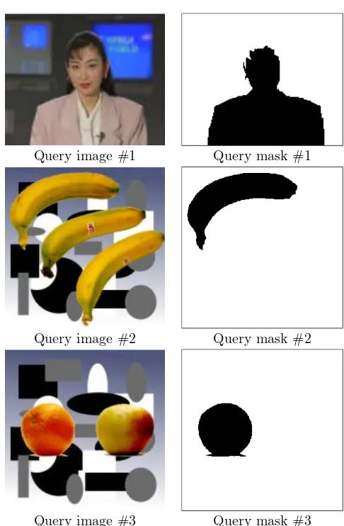
Query image #1 Query mask #1
Query image #2 Query mask #2
[image:33.595.164.407.108.479.2]Query image #3 Query mask #3
Figure 6.7: Query regions for the single query region. The query region is defined via the query image and query mask.
discussed, the search through the database is done in a sequential manner for all the trees in the database. The dissimilarity of the nodes of each tree with respect the query are analyzed using Eq. 6.4. The weights associated to the distances in Eq.6.4are set to ωi= 1/4, that is,
every descriptor receives the same importance.
Moreover, the query images have been included in the database. As a result, each query should appear at the first positions of the initial positions for corresponding retrieved results. It should be noted that the query does not have to appear necessarily at the first position. This issue will be discussed afterwards.
#01 – akiyo 01 #02 – akiyo 02 #03 – akiyo 04 #04 – akiyo 03
[194] 0.015358 [197] 0.042920 [197] 0.043529 [195] 0.044795
#05 – akiyo 01 #06 – akiyo 05 #07 – akiyo 04 #08 – akiyo 05
[197] 0.046055 [197] 0.048004 [194] 0.068386 [194] 0.069542
#09 – akiyo 02 #10 – akiyo 04 #11 – akiyo 05 #12 – miss 02
[194] 0.072896 [191] 0.115963 [192] 0.119275 [198] 0.121384
#13 – miss 01 #14 – akiyo 02 #15 – akiyo 03 #16 – claire 01
[198] 0.122436 [193] 0.123764 [193] 0.124366 [198] 0.127326
#17 – miss 03 #18 – claire 12 #19 – claire 11 #20 – claire 02
[image:34.595.100.518.117.659.2][198] 0.130856 [198] 0.131975 [198] 0.132719 [198] 0.136393
#01 – ima 08 #02 – ima 08 #03 – ima 08 #04 – ima 08
[183] 0.002407 [172] 0.090976 [181] 0.096731 [176] 0.131378
#05 – ima 08 #06 – ima 08 #07 – ima 17 #08 – ima 08
[150] 0.147846 [161] 0.156220 [184] 0.159911 [154] 0.160528
#09 – ima 18 #10 – ima 08 #11 – ima 08 #12 – ima 20
[181] 0.163623 [146] 0.166526 [182] 0.168021 [178] 0.168260
#13 – ima 16 #14 – ima 19 #15 – ima 11 #16 – ima 11
[181] 0.168260 [183] 0.168637 [194] 0.176896 [187] 0.181004
#17 – ima 21 #18 – ima 08 #19 – ima 08 #20 – bream 200
[image:35.595.109.463.121.658.2][179] 0.182268 [126] 0.189607 [153] 0.192474 [195] 0.199136
#01 – ima 001 #02 – ima 003 #03 – ima 019 #04 – ima 018
[185] 0.002120 [184] 0.049541 [187] 0.054108 [184] 0.054108
#05 – ima 017 #06 – ima 016 #07 – ima 020 #08 – ima 002
[186] 0.054108 [187] 0.054108 [182] 0.054130 [184] 0.058698
#09 – ima 005 #10 – ima 004 #11 – ima 007 #12 – ima 021
[189] 0.074799 [189] 0.087654 [182] 0.102911 [184] 0.104432
#13 – ima 001 #14 – ima 007 #15 – ima 006 #16 – ima 007
[169] 0.119748 [179] 0.124723 [187] 0.129957 [181] 0.143856
#17 – ima 003 #18 – ima 007 #19 – ima 001 #20 – ima 001
[173] 0.149751 [171] 0.153710 [143] 0.153738 [155] 0.165109
#01 – akiyo 01 #02 – claire 01 #03 – miss 01 #04 – claire 05
[194] 0.040365 [198] 0.053408 [198] 0.060594 [198] 0.068408
#05 – claire 11 #06 – claire 12 #07 – claire 02 #08 – akiyo 01
[198] 0.069109 [198] 0.069388 [198] 0.071222 [197] 0.071726
#09 – akiyo 02 #10 – akiyo 04 #11 – claire 03 #12 – claire 04
[197] 0.072048 [197] 0.074516 [198] 0.079974 [198] 0.082525
#13 – claire 09 #14 – claire 10 #15 – miss 02 #16 – claire 08
[198] 0.084320 [198] 0.085330 [198] 0.088479 [198] 0.091927
#17 – miss 03 #18 – news 05 #19 – claire 07 #20 – akiyo 05
[198] 0.092282 [197] 0.093189 [198] 0.093674 [197] 0.095993
Figure 6.11: Query results for query region #1 defined in Fig. 6.7. Weights have been set as following: ωshape = 1 and ωhisto = ωsize = ωpos = 0. For each item of the result, its
akiyo and claire images included in the database, whereas no mask has been used in the case of miss america. As a result, the region of support of the akiyo and claire newscaster are represented as a node in its associated tree representations and can be retrieved as such, for instance see items #2, #3, #19 and #20. On the other hand, in the case of the miss america we cannot make sure that the region of support of the woman is represented as a node in its associated tree representation. In fact, the analysis of its tree representations associated to the miss america images included in the database shows us that the regions associated to the hair and arms of the woman are merged with the background during the creation of the tree due to its high color similarity with respect the background. As a result, the miss america regions can be only retrieved as shown in items #12, #13 and #17.
Moreover, the query appears at the the first position in the retrieval results. However, the region of support of the query mask #1 and the one shown in item #1 of Fig.6.9are dissimilar. This is due to the fact that the region of support of the query mask is not represented as a node in the corresponding tree included in the database. The tree included in the database has been constructed forcing the support of the region associated to the newscaster (by means of a mask), whereas the query mask #1 has been defined by means of the marker & propagation algorithm of Sec. 5.7.1 using a tree that has been constructed based on color homogeneity. Both trees are different and the regions of support of its associated regions also are different.
Fig. 6.9 (resp. Fig. 6.10) shows the results of the retrieval using query #2 (resp. query #3). The retrieved regions correspond to bananas (resp. oranges and apples) visually similar to the query. As in the previous example, the search engine retrieves similar objects present in the database by giving each of the descriptors the same importance. The search engine is able to retrieve some relevant objects present in the database. Moreover, note that some items in the retrieval results are associated to a descendant node of another item also present in the retrieval result.
However, as already discussed, it has to be noted that manually setting the weights is not always simple. In general, it is not easy to manually map the users need to numerical values of the weights associated to the descriptors. This mapping gets harder as the number of available descriptors increases. Moreover, we cannot assume that a user having no technical knowledge of content based retrieval is able to manually set these weights. For that purpose a relevance feedback approach is presented in Sec.6.7.
6.6
Multiple region query
6.6.1 Query strategy
In Sec.6.5, a method for searching single regions in Binary Partition Trees has been presented. This section is devoted to the extension of the approach to multiple regions. The user provides the search engine with the query object (masks and pixels values) to search for. Note than in this case the query object is made up of several unconnected regions. The search engine looks for a set of regions in the Binary Partition Trees of the database taking into account their visual similarity and their relative positions and sizes with respect the query. That is, we have to take into account the structural relationship between the regions to search for. For notation purposes, let us denote withQ the query object which is made up of the query regions Qi, Q = {Qi} with 1 ≤ i ≤ NRQ, where NRQ is the number of regions the query
object is made up of. Let us denote with T the target object which is also made up ofNRQ
target regions, T = {Tj}, 1 ≤ j ≤ NRQ. For simplicity, the distance between Q and T is
assessed by assuming that Q1 is matched against T1,Q2 against T2, and so on.
The problem, discussed in this section, is how to efficiently find a set of target objectsT in the set of trees composing the database. A simple solution would consist in generating, for each tree in the database, all possible target objects T by generating all combinations of the nodes that composes the tree. The target objects could then be ordered according to is similarity with respect the query. This brute force solution is computationally very expensive and thus a suboptimal algorithm has been developed (Sec. 6.6.6).
6.6.2 Query object normalization
In order to be able to measure the structural distance between the query and target, the query object has to be properly scaled. Fig. 6.12 shows an example of query and target object having a similar structural relationship. Both objects are made up of three regions, each region is represented with a node. The cross in (resp. radius of) each node is associated to its associated position (resp. size) descriptor. Observe that both objects cannot be compared if the query object is not scaled properly to the size of the target.
Q1
T1
Query object Target object
Figure 6.12: Example illustrating the need of query object normalization for comparison purposes.
the query object Q and the target object T. The purpose of query normalization is to scale properly Q to the scale of the target T. More formally, the purpose of the query object normalization is to scaleDpos(Qj) andDsize(Qj) using a target regionTi as reference.
Normalization is done by warping the query object Q over the target object T using Ti as
reference region. The normalized position and size descriptors of the query region,DN pos(Qj)
andDNsize(Qj), are interpreted as the “ideal” position and size descriptors the target regions
should fulfill.
The approach taken in this work to perform query object normalization can be easily explained using Fig. 6.13. On the left, the query object Q, made up of three regions, is shown. Each region is represented with a node.
Assuming that reference region Ti is known (for instance, T2 in Fig. 6.13), the first step
in the normalization is to obtain the centroid of the normalized query object,CN
Q, by means
of the centroid of the query object Q and the position and size descriptor associated to Ti.
The centroid of the query object,CQ, is obtained as:
CQ =
1 NRQ
NRQ
X
j=1
Dpos(Qj)
The centroid of the normalized query object,CN
Q, is obtained as follows:
CQN =Dpos(Ti) + (CQ−Dpos(Qi))× Dsize(Ti)
Dsize(Qi)
Note thatDsize(Ti) and Dsize(Qi) are scalar values, whereasDpos(Ti), Dpos(Qi) and CQ are