Sequential Detection of Artifacts in Electroencephalographic Signals using Nonparametric Statistical Methods-Edición Única

(1)

Monterrey, Nuevo León a

INSTITUTO TECNOLÓGICO Y DE ESTUDIOS SUPERIORES DE MONTERREY

PRESENTE.-cual autorizo a el Instituto Tecnológico y de Estudios Superiores de Monterrey (EL INSTITUTO) para que efectúe la divulgación, publicación, comunicación pública, distribución, distribución pública y reproducción, así como la digitalización de la misma, con fines académicos o propios al objeto de EL INSTITUTO, dentro del círculo de la comunidad del Tecnológico de Monterrey.

El Instituto se compromete a respetar en todo momento mi autoría y a otorgarme el crédito correspondiente en todas las actividades mencionadas anteriormente de la obra.

De la misma manera, manifiesto que el contenido académico, literario, la edición y en general cualquier parte de LA OBRA son de mi entera responsabilidad, por lo que deslindo a EL INSTITUTO por cualquier violación a los derechos de autor y/o propiedad intelectual y/o cualquier responsabilidad

(2)

Sequential Detection of Artifacts in Electroencephalographic

Signals using Nonparametric Statistical Methods-Edición Única

Title Sequential Detection of Artifacts in

Electroencephalographic Signals using Nonparametric Statistical Methods-Edición Única

Authors Carlos Alejandro Robles Rubio

Affiliation Tecnológico de Monterrey, Campus Monterrey

Issue Date 2008-11-01

Item type Tesis

Rights Open Access

Downloaded 19-Jan-2017 02:57:36

(3)

Sequential Detection of Artifacts in

Electroencephalographic Signals using

Nonparametric Statistical Methods

Carlos Alejandro Robles Rubio

Division of Mechatronics and Information Technology

Instituto Tecnol´ogico y de Estudios Superiores de Monterrey

Monterrey, Nuevo Le´on, M´exico

November 2008

A thesis submitted to the Instituto Tecnol´ogico y de Estudios Superiores de Monterrey, Campus Monterrey, in partial fulfillment of the requirements for the degree of Master of

Science in Electronic Engineering (Electronic Systems).

c

(4)

Instituto Tecnol´ogico y de Estudios Superiores de Monterrey Campus Monterrey

Graduate Program in Engineering

Division of Mechatronics and Information Technology

Sequential Detection of Artifacts in Electroencephalographic Signals using Nonparametric Statistical Methods

by Carlos Alejandro Robles Rubio

Dr. Frantz Bouchereau Lara Thesis Advisor

Dr. Sergio Omar Mart´ınez Chapa Thesis Co-advisor

Dr. Graciano Dieck Assad Synodal

Dr. Joaqun Acevedo M.

Director of the Graduate Program

Date: November 15, 2008.

The members of the thesis committee hereby approve the thesis of Carlos Alejandro Robles Rubio as a partial fulfillment of the requirements for the degree of Master of

(5)

(6)

(7)

(8)

Abstract

(9)

(10)

Resumen

(11)

(12)

Acknowledgments

I would like to thank the Instituto Tecnol´ogico y de Estudios Superiores de Monterrey for the institutional and financial support on the development of my masters degree studies. Similarly I thank the BioMEMS research group and its coordinator, Dr. Sergio Omar Mart´ınez Chapa for the offered financial support and the opportunity to collaborate in the electroencephalography research project. I also thank Dr. Mart´ınez, who acted as my thesis co-advisor, for his comments and reviews on the final stage of this work.

I also want to thank my thesis advisor Dr. Frantz Bouchereau Lara for all his comments, reviews and guidance through the inception and development of this research work. To the synodal of the thesis committee Dr. Graciano Dieck Assad, for his review and highlights on this document.

I am truly grateful to my parents Carlos Salvador and Susana and my sister Paulina for their love, affection and support during all the steps in my life, which led me to the culmination of this degree.

I am thankful to M.C. Ana Cecilia Puón D´ıaz, M.C. Victor Hugo Pérez González and M.C. Juan Alberto González Lugo for their friendship, help and collaboration during the development of the novel methods described in this thesis. I specially thank Ana Cecilia for her support, affection and love that helped me during this period of studies.

I would like to manifest my appreciation to my friends and colleagues Alejandro, Anto-nio, Carlos, Carolina, Christian, Deneb, Edgardo, Enrique, Ernesto, Héctor, Igmar, Jorge, José Luis, Julián, Liliana, Luis, Lyz, Manuel, Marco, Miguel, Omar, Ramón, Raúl, Rodolfo, Rubén, Sandra, Stephanie and Zu-Lym for their support and friendship and the convivial-ity during my studies of the masters degree.

(13)

(14)

List of Figures

2.1 Action potential general schema (adopted from S. Sanei [1]) . . . 7

2.2 Comparisson of the waveforms of the typical brain rhythms (adopted from [1]) 9 2.3 Example of a multichannel EEG with the occurrence of a tonic-clonic (grand mal) seizure (adopted from [1]) . . . 11

2.4 The 10-20 standard for electrode location in EEG . . . 13

2.5 Example of a multichannel EEG with the occurrence of an OA (adopted from [1]) . . . 18

5.1 Example of a Simulated EEG signal ˆu1[n] . . . 45

5.2 Segment of EEG signal ucba1f f01,O2[n] . . . 46

5.3 Segment of EEG signal ucba1f f01,T5′[n] . . . 47

5.4 Segment of artifactual signals with individual artifacts of length L = 250. a) White noise, b) Sawtooth, c) Mixed ECG and EMG, d)Simulated ECG 49 5.5 Curve of ROC #1 for the evaluation of the BSM. See Table 5.1 . . . 52

5.6 Curve of ROC #2 for the evaluation of the BSM. See Table 5.1 . . . 53

(17)

List of Figures xiv

5.17 Curve of ROC #13 for the evaluation of the BSM. See Table 5.1 . . . 67 5.18 Curve of ROC #14 for the evaluation of the BSM. See Table 5.1 . . . 68 5.19 Curve of ROC #15 for the evaluation of the BSM. See Table 5.1 . . . 69 5.20 Curve of ideal ROC with the BSM for the evaluation of the CCDA detector 72 5.21 Curve of ROC with the BSM and estimated AR parameters for the

evalua-tion of the CCDA detector . . . 74 5.22 Curve of ROC with the BSM and true EEG signal ucba1f f01,O2[n] for the

evaluation of the CCDA detector . . . 76 5.23 Curve of ROC with the BSM and true EEG signal ucba1f f01,T5′[n] for the

evaluation of the CCDA detector . . . 78 5.24 Curves of probability of detection and probability of false alarm when the

parameter L′ _{is variated and the input signal is ˆ}_u

1[n] . . . 80

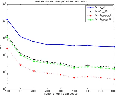
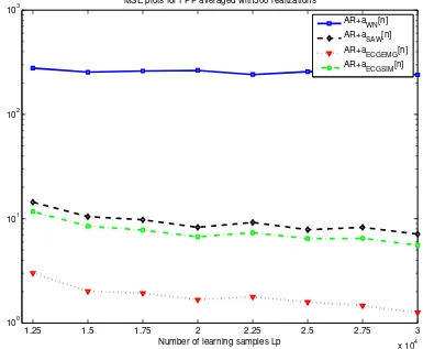
5.25 Curves of MSE when applying FPP to the ideal AR process for threshold estimation with Q=500 realizations . . . 83 5.26 Curves of MSE when applying BR to the ideal AR process for threshold

estimation with Q=500 realizations . . . 84 5.27 Curves of MSE when applying FPP to an AR process withL′ _learning

sam-ples for threshold estimation with Q=5000 realizations . . . 85 5.28 Curves of MSE when applying BR to an AR process withL′_{learning samples}

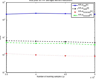
for threshold estimation with Q=500 realizations . . . 86 5.29 Curves of MSE when applying FPP to an AR process withL′ _learning

sam-ples for threshold estimation with Q=500 realizations . . . 87 5.30 Curves of MSE when applying FPP to an AR process withL′ _learning

sam-ples for threshold estimation with Q=500 realizations . . . 88 5.31 Curves of MSE when applying FPP to an AR process withL′ _learning

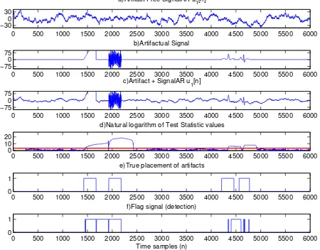
sam-ples for threshold estimation with Q=500 realizations . . . 89 5.32 Online performance of CCDA with ideal threshold and ideal AR parameters 90 5.33 Online performance of CCDA with FPP estimated threshold from L′ _{= 250}

samples and AR signal ˆu[n] . . . 91 5.34 Online performance of CCDA with FPP estimated threshold from L′ ₌

2_×105 _{samples and AR signal ˆ}_u_[_n_{] . . . .} ₉₂

5.35 Online performance of CCDA with BR estimated threshold from L′ _{= 250}

(18)

5.36 Online performance of CCDA with BR estimated threshold fromL′ _{= 2}_×₁₀5

samples and AR signal ˆu[n] . . . 94 5.37 Online performance of CCDA with FPP estimated threshold from L′ _{= 250}

samples and true EEG signal ucba1f f01,O2[n] . . . 95

5.38 Online performance of CCDA with FPP estimated threshold from L′ ₌

2_×105 _{samples and true EEG signal} _u

cba1f f01,O2[n] . . . 96

5.41 Online performance of CCDA with FPP estimated threshold from L′ _{= 250}

samples and true EEG signal ucba1f f01,O2[n] and model order M = 7 . . . . 99

5.42 Online performance of CCDA with FPP estimated threshold from L′ ₌

2_×105 _{samples and true EEG signal} _u

cba1f f01,O2[n] and model order M = 7 100

5.45 Online performance of CCDA with FPP estimated threshold from L′ _{= 250}

samples, true EEG signal ucba1f f01,O2[n], model orderM = 7 andPF A = 0.1 103 5.46 Online performance of CCDA with BR estimated threshold from L′ _{= 250}

samples, true EEG signal ucba1f f01,O2[n], model orderM = 7 andPF A = 0.1 104

B.1 Curve of ROC #1 for the evaluation of the BSM for a less correlated AR than the one used in chapter 5. See Table 5.1 . . . 118 B.2 Curve of ROC #2 for the evaluation of the BSM for a less correlated AR

than the one used in chapter 5. See Table 5.1 . . . 119 B.3 Curve of ROC #3 for the evaluation of the BSM for a less correlated AR

(19)

List of Figures xvi

B.6 Curve of ROC #6 for the evaluation of the BSM for a less correlated AR than the one used in chapter 5. See Table 5.1 . . . 123 B.7 Curve of ROC #7 for the evaluation of the BSM for a less correlated AR

(20)

List of Tables

2.1 Most common types of epileptic seizures and their characteristics [1] . . . . 17

5.1 Moments used to find the most appropriate ROC . . . 50 5.2 Data for the calculation of the BSM using the sets defined in Table 5.1 . . 70 5.3 Data from the Ideal ROCs evaluation . . . 73 5.4 Data from the ROCs evaluation of signalucba1f f01,O2[n] . . . 77

5.5 Data from the ROCs evaluation of signalucba1f f01,T5′[n] . . . 77

5.6 Data from the ROCs evaluation of signals ˆu[n],ucba1f f01,O2[n] anducba1f f01,T5′[n] 79

A.1 Computational cost of CCDA procedures in terms of combined multiplica-tion and sum operamultiplica-tions . . . 115

(21)

(22)

List of Acronyms

ADC Analog to Digital Converter AEEG Ambulatory EEG

AP Action Potential AR Autoregressive AuROC Area under the ROC

BioMEMS Biological Micro Electro-Mechanical Systems BR Bootstrap Resampling

BSM Best Set of Moments BSS Blind Source Separation

CCDA Central Chi-Square Detection Algorithm CNS Central Nervous System

DI Data Improbability ECG Electrocardiogram EEG Electroencephalogram EKG Electrocardiogram EMG Electromyogram EOG Electrooculogram ERP Event Related Potential

EV Extreme Values

fMRI Functional Magnetic Resonance Imaging FPP Forward Prediction Pseudo-sampling IC Independent Component

(23)

List of Terms xx

ITESM Instituto Tecnol´ogico y de Estudios Superiores de Monterrey LMS Least Mean Square

LT Linear Trends

MSE Mean Squared Error

NCDA Non-Central Chi-Square Detection Algorithm OA Ocular Artifact

PCA Principal Component Analysis PDF Probability Distribution Function pdf Probability Density Function RLS Recursive Least Squares

ROC Receiver Operating Characteristics SP Spectral Pattern

(24)

Chapter 1 Introduction

This research project is developed in the area of Electroencephalographic (EEG) Signal Pro-cessing. Currently most EEG studies are made in dedicated facilities, which are generally located at hospitals, laboratories and specialized clinics, due to the necessary equipment and the required controlled environment where they should be performed. This is to reduce occurrence of noise that could lead to a wrong representation of data and consequently to their misinterpretation. The design of ambulatory EEG systems facilitates these proce-dures, giving the patients the opportunity to stay at their day to day environment (i.e. home, office, etc.), eliminating the hospital cost, and permitting the generation of longer recordings. Besides this, some of the problems that provoke the symptoms of the patient may be related directly with the day to day life activities rather than with controlled en-vironments, which is another important reason for the development of ambulatory EEG (AEEG) systems [2].

(25)

1 Introduction 2

1.1 Problem Description

The signals obtained with an electroencephalogram not only show the brain activity, but also some other electric potentials generated by the activity of another organs. These signals are called artifacts, and the segments of EEG recorded data that contain them have to be discarded. Nowadays there is research in the cancellation of artifacts, reconstruction of EEG signals, their spectrum analysis, and certain work related with detection of artifacts like encountered in references [3] and [4]. The main drawback of these detection techniques is that they are not designed for the detection of several kind of artifacts, and also that they require a priori knowledge of the statistics of the clean EEG signal and the artifacts being detected.

1.2 Objective

The general objective of this research work is to develop, research and test efficient algo-rithms for the sequential detection of artifacts in EEG signals, considering that there is no previous knowledge of the artifact characteristics and based on the statistical signal processing techniques.

The scope of this project is limited to the detection of artifacts in the EEG signals, giving the opportunity to perform their cancelation and also to implement them in a hardware platform for future research work.

1.3 Justification

The importance of considering the mentioned problem when working with EEG signals arises from the need of the neurologists to find certain parameters and behaviors that help to clarify the health state of the patient. However in the presence of contaminated data sections it is not possible for them to correctly analyze the information. Moreover, these tests require adequate equipment to avoid subsequent repetitions due to data acquisition problems which could derive in additional cost, time and inconvenience to patients.

(26)

resources, because as in every embedded system, there is the need to optimize the algorithms in order to implement them online and in real time. Identifying each artifact by its wave form, spectrum and statistics in order to program it in a portable system, requires very large amount of memory, besides it implies high processing work. This is why having a technique capable of recognizing artifacts based on common characteristics is of great utility.

1.4 Contribution

The contribution of this work is the development of a novel method for the sequential de-tection of artifacts in EEG signals, by means of nonparametric statistical methods. The detector can be tuned for the detection of any type of artifact and it can work with both raw EEG data or EEG after BSS (e.g. independent components from ICA). This methodology does not need a priori knowledge neither of the clean EEG statistics nor of the EEG plus artifact characteristics, it only needs a few learning samples to deliver results. The method is composed of three steps: process and detector characterization, adaptive threshold esti-mation, and sequential implementation. Several approaches are presented and developed for the three steps. The performance analysis of the first step is fully tested and character-ized, the second is tested with an ideal random process, and the analysis of the capabilities of the last one is left as future research work.

1.5 Thesis Organization

(27)

(28)

Chapter 2 EEG Background

2.1 Electroencephalogram Basics

An electroencephalogram consists on a set of measurements taken from the scalp or the brain by means of electrodes, that correspond to the electrical neural activity. In the early days of the electroencephalography the recordings where taken with few electrodes, but nowadays the signals are taken with an array of multiple sensors and using fully comput-erized systems, which are equipped with signal analysis and processing tools and enough memory for long time recording. If the data is taken directly from the brain it is called an electrocortiogram [1, 5].

(29)

2 EEG Background 6

2.1.1 Electroencephalogram Generation

The information transmitted by the nerves is called an action potential (AP) and it is gen-erated by an exchange of ions through the structure of the neurons and their connection with other neurons by means of the axons and dendrites which are part of these nervous system cells. The velocity of this communication is from about 1 to 100 m/s, and these events are generated by stimuli like chemical, light, electricity, pressure, touch and stretch-ing in sensory nerves, and primarily by chemical activity in the central nervous system (CNS, brain and spinal cord). It is important to remark that a stimulus must surpass certain threshold in order to trigger an AP. For a person the amplitude of the AP ranges between approximately ₋60mV and 10mV. The potential before polarization is of about

−70mV, but by the stimulus of ions the charge becomes less negative and if it reaches limit of₋55mV the AP process continues. The potential may reach +30mV in the AP peak and then the depolarization takes the signal down to an undershoot of approximately ₋90mV, called hyperpolarization, and finally to the settling state of ₋70mV, see Figure 2.1. The hyperpolarization prevents the neuron from receiving any other stimulus during this time [1].

When several neurons are activated, they generate currents within their communication channels. This current generates a magnetic field that can be read by an electromyogram (EMG) machine, and also a secondary electrical field over the scalp which is what the EEG is able to measure and record. Due to the electric resistance of the human head, generated mainly by the brain, skull and scalp, only potentials generated by a large population of active neurons can be obtained with scalp electrodes. After their acquisition, the signals are amplified for either display or processing purposes [1].

According to [1] the study of EEGs aids in the diagnosis of many neurological disorders and abnormalities in the human body. These signals may be used for research on the following:

• monitoring alertness, coma, and brain death;

• locating areas of damage following head injury, stroke, and tumour;

(30)

[image:30.612.163.547.107.390.2]

Fig. 2.1 Action potential general schema (adopted from S. Sanei [1])

• monitoring cognitive engagement (alpha rhythm);

• producing biofeedback situations;

• controlling anesthesia depth (servo anesthesia);

• investigating epilepsy and locating seizure origin;

• testing epilepsy drug effects;

(31)

2 EEG Background 8

• monitoring brain development;

• testing drugs for convulsive effects;

• investigating sleep disorders and physiology;

• investigating mental disorders;

• providing a hybrid data recording system together with other imaging modalities.

2.1.2 Brain Rhythms and Abnormal Epileptic EEG Paterns

The EEG signals have characteristic patterns that appear in certain frequency bands. Those patterns are called brain rhythms and are classified by their frequency domain. The main brain waves are called alpha (α), theta (θ), beta (β), delta (δ), and gamma (γ) [1].

The theta waves are in the range of 4-7.5Hz. These waves appear as consciousness slips towards drowsiness, and they have been associated with access to unconscious material, creative inspiration and deep meditation. Larger contingents of theta wave activity in the waking adult are abnormal and are caused by various pathological problems [1].

Alpha rhythms appear in the posterior half of the head and are found over the occipital region. Their characteristic frequency range lies within 8-13Hz and has the appearance of a round or sinusoid-like signal. It has an amplitude of normally less than 50µV and it can be found in the occipital area of the head. This rhythm has been thought to indicate both a relaxed awareness without any attention or concentration. In general, the alpha waves appear with eyes closed and they are reduced or disappear by opening the eyes, hearing unfamiliar sounds, anxiety or mental concentration. The origin and physiological signifi-cance of alpha waves is still unknown and yet more research is needed in the area [1].

(32)

[image:32.612.142.503.204.504.2]

In the range above 30Hz lies the gamma rhythm, also called the fast beta wave. Its amplitudes are very low and it has a rare occurrence, but this rhythm can be used for con-firmation of certain brain diseases. It can be mainly located in the frontocentral area of the head. This band has been proved to be a good indication of event-related synchronization of the brain. Figure 2.2 shows a comparisson of the typical waveforms for the mentioned brain rhythms [1].

Fig. 2.2 Comparisson of the waveforms of the typical brain rhythms (adopted from [1])

(33)

2 EEG Background 10

for several purposes like the treatment of epileptic seizure disorder [1].

There are several mental disorders that may provoke the apparition of abnormal pat-terns in the EEG, mainly due to the changes in the network of neurons and the variations on their communication. Some examples of these problems are aging, dementia, epilepsy, psychiatric disorders (e.g. attention-deficit disorder) among others. Abnormal patterns may also arise from external effects such as looking at the TV screen, listening to music without any attention or also pharmacological and drug effects [1].

On the specific case of epilepsy, it comprises a diverse collection of disorders. The most common therapy is symptomatic, and the available drugs reduce the frequency of the seizures in the patients, but only a low percentage are free of them. The termseizure refers to a transient change of behavior due to the disordered, synchronous and rhythmic firing of populations of CNS neurons, and epilepsy is defined as a disorder of brain function charac-terized by the occurrence of recurrent, unpredictable and non induced seizures. When the seizures are intentionally provoked they are considered nonepileptic. The terms ictal and interictal refer to the adjectives “seizure-like” and “between seizure” respectively [7].

The behavioral manifestations of a seizure appear in the functions normally served by the cortical region where the seizure arises. When a simple partial seizure occurs the person generally preserves consciousness, on the other hand, a complex partial seizure is associated with impairment of consciousness. The majority of the last mentioned seizures originate in the temporal lobes. Absence, myoclonic, and tonic-clonic are examples of generalized seizures. A given patient usually exhibits multiple kinds of seizures in different episodes [7]. For further details in the classification and explanation on epileptic seizures and the common patterns in which they appear refer to [8].

Studies performed in EEG recordings for different kind of seizures reveal that there are distinctive abnormalities for different kind of seizures, e.g. there are patterns for tonic seizures and they differ from those of a clonic seizure [7]. Figure 2.3 shows a multichannel EEG with a generalized tonic-clonic (grand mal) seizure.

(34)

Fig. 2.3 Example of a multichannel EEG with the occurrence of a tonic-clonic (grand mal) seizure (adopted from [1])

shows the most common kinds of seizures and their characteristics [1].

(35)

2 EEG Background 12

The distinction of epileptic seizure from common artifacts can be made based on the repetitive (rhythmical) nature of the epileptic spikes, which is different from the artifacts that are transients or noise-like in shape. In the specific case of electrocardiogram (ECG) the frequency of occurrence of the waveforms is approximately 1 Hz, but this waves are very different in shape compared with the seizure signals [1].

There may be spikes and other paroxysmal discharges in nonepileptic persons, and they may be found in healthy individuals; however they usually are signs of certain cerebral dysfunctions that may or may not develop into an abnormality. They may appear during periods of particular mental challenge on individuals, like soldiers in the war, pilots and prisoners [1].

2.1.3 EEG Measurement

The most used international standard for the collocation of the electrodes in EEG record-ings is the 10-20 system, and it has 21 record points. The arrangement uses two points as reference, the Nasion, that is just above the nose in line with the eyes, and the Inion, found in the bone that is in the posterior base of the skull. From the reference points, the electrodes are positioned separated each 10 or 20% of the head surface. For a graphic representation of this array, see Figure 2.4. The amplitude of these signals is near 100µV if observed from the scalp, and from 1 to 2mV when recorded from the brain surface. The bandwidth is from 1 to 50Hz approximately [5, 1].

Commercial EEG recording systems frequently include impedance monitors to maintain an adequate level in this parameter because high impedance can lead to distortion in the signals [1].

(36)

Fig. 2.4 The 10-20 standard for electrode location in EEG

sampling frequencies for EEG recordings are 100, 250, 500, 1000, and 2000 samples/s [1]. There are several methods to eliminate or mitigate the effects of the power line frequency interference, from a notch filter with null frequency in 50 or 60Hz to adaptive noise cancelers like the one described in [9].

2.2 Artifacts

(37)

2 EEG Background 14

Due to their specific characteristics, the ocular artifacts (OA) like eye blinks are par-ticularly difficult to locate and eliminate from the EEG signals without losing important information of event-related potentials (ERPs). This kind of artifact generates signals within EEG of the order of ten times larger in amplitude than the cortical signals and last from 200 to 400 ms. This fact will be used later for the design of test cases for the different algorithms described within this text. Due to the power of the blinking artifacts and the scalp’s resistance the OAs can affect a large part of the electrodes. Figure 2.5 shows an example of the EEG signals with an OA [11, 12, 1].

Another common type of artifactual signal is the ECG, it occurs when the cardiac elec-trical field affects the potentials on the scalp and near the eyes. It leads to interference in the EEG and EOG recordings, and it can be easily recognized by its periodicity and coincidence with the ECG channel peaks. Its waveform varies from time to time, and large inter-individual voltage variations can be observed [13]. The work in [14] analyses this kind of artifact when a subject is under a functional Magnetic Resonance Imaging analysis (fMRI), where it commonly has more severe impact in the EEG signal; and the artifactual amplitude, spatial distribution on the scalp and frequency of occurrence is investigated. Their results show that this interference is normally largest in the frontal region, and that the mean amplitude of the artifact (from 78 channels in total) was 58µV with standard de-viation SD = 58µV when the electrode leads were untwisted, and 36µV with SD = 34µV when the leads were twisted together. These results will be used in section 5.1.2 for the generation of test artifacts.

(38)

2.2.1 Previous work with artifacts in EEG

One of the most predominant artifact rejection research lines is the use of Independent Component Analysis (ICA), which is a technique of the branch of blind source separa-tion analysis (BSS). It performs a decomposisepara-tion from observed multichannel signals into various independent components, looking for statistical independency, not only based in decorrelation, but also in high-order statistical independence which is what makes it dif-ferent from Principal Component Analysis (PCA) [16]. The main problem with ICA is that for EEG, the number of sources is not easily found thus almost all of the indepen-dent components obtained may contain important EEG data that should not be ignored for clinical analysis; and ICA relies in the assumption that the number of sensors is equal to the number of independent components, which is difficult to achieve [17]. Works using ICA include [3, 13, 16, 17, 18, 19, 20, 21]. In [17] an alternative to ICA for EEG artifact correction without the assumptions of this BSS method is presented.

The detection method presented in this work can be used after ICA decomposition, but it is mainly intended for use with reconstruction methods like the one described in [17], where the algorithms work directly with the EEG data.

(39)

2 EEG Background 16

within the EEG signal.

The work of [22] assumes that the EEG signal can be modeled with an AR process, and it uses the variance of the innovation (by inverse filtering the EEG after estimating the AR parameters) as an indicator of the presence or absence of artifacts. It is thought from the perspective that the EEG is a stationary process within a segment of time, and thus the variance of the innovation is relatively constant. If this variance presents a significant change, it is said to be an EEG signal with artifactual contamination.

From another point of analysis, the method in [23] is based on the Wavelet Transform (WT), and it is intended to eliminate ECG artifacts based on their characteristic spectral content.

In [21] the authors introduce the Hurst exponent as an indicator of the presence or absence of artifactual signals in the EEG. According to this work, a time series can be parametrized by means of the Hurst exponent, and it has been found that this parameter H has a value equal to 0.70₋0.76 for many natural, economic and human phenomena. With respect to artifactual signals, the ECG artifact has a value in the range ofH = 0.64₋0.69 and the eye blinking or OA is in the range of H = 0.58₋0.64. The method consists on performing ICA for ICs separation and then calculating the corresponding Hurst exponent to yield a decision. Taking this categorization into account, the signal subspace is obtained and the data is filtered to obtain the corrected EEG signal. The work presents the method for the Hurst exponent recurrent calculation, enabling it to be used in sequential online processing. The main drawback of this method is that it relies on the ICA assumptions, and also that it needs certain a priori information about the characteristic values of the Hurst exponent for each of the signals that it wants to detect.

(40)

Table 2.1 Most common types of epileptic seizures and their characteristics [1]

Kind Spatial location Frequency Description Tonic-clonic All electrodes

with tendency to frontal ones

6-12 Hz It is the most common type of epileptic seizure and it has a rhythmic but spiky pattern in the EEG.

Petit-mal - 3 Hz Interictal paroxysmal seizure with a gen-eralized synchronous spike wave complex of prolongued bursts.

Psychomotor Temporal lobe 4-6 Hz Also called complex partial seizure. It is presented by bursts of serrated slow waves with amplitude of above 60 µV. Cortical(focal) - - Rising amplitude and diminishing

fre-quency during ictal period. It is usually initiated by local desynchronization. Myoclonic Frontal region - Concomitant polyspikes, seen clearly in

the EEG. They can have generalized or bilateral spatial distribution.

Tonic - 10 Hz Occur in patients with Lennox-Gastaut

syndrome and have spikes that repeat at the given frequency.

Atonic Generalized 1-2, 10 Hz May appear in the form of a few sec-onds drop attack or be inhibitory, last-ing for a few minutes. They show a few polyspike waves or spike waves with gen-eralized spatial distribution followed by large slow waves.

Akinetic - 1-2 Hz It is a rare kind of seizure and it is char-acterized by arrest of all motion but it is not caused by a sudden loss of tone as in atonic seizure. The patient is in an absent-like state.

(41)

2 EEG Background 18

(42)

Chapter 3 Theoretical Background

3.1 Autoregressive Random Process Model

An Autoregressive (AR) sequence is a time series that can be used to model certain random processes, and it can be defined as

x[n] =₋ M

X

i=1

aix[n−i] +ǫ[n] (3.1)

whereǫ[n]_∼N(0, σ2

ǫ) is the driving noise of the sequence,x[n] is the random variable in timen andM is the order of the AR sequence. An important remark is that the values ofǫ at each time ncome as a random sample, i.e. they are independent and equally distributed [24].

A relevant aspect of the AR processes is the relation of the AR coefficients a with the lags of the autocorrelation sequencer(l). This relation is given by the Yule-Walker equation by the following equation



    

r(0) r(₋1) . . . r(₋M+ 1) r(1) r(0) . . . r(₋M+ 2)

... ... . .. ...

r(M ₋1) r(M ₋2) . . . r(0)



    



    

−a1

−a2

...

−aM



    

=



    

r(₋1) r(₋2)

... r(₋M)



    

(3.2)

(43)

3 Theoretical Background 20

are the values of the AR parameters [24]. For real valued processes the autocorrelation sequence is symmetric with respect to the origin, i.e. r(0), and the Yule-Walker equations become      

r(0) r(1) . . . r(M ₋1) r(1) r(0) . . . r(M ₋2)

... ... . .. ...

r(M ₋1) r(M ₋2) . . . r(0)

           

−a1

−a2

...

−aM

      =       r(1) r(2) ... r(M)

      (3.3)

The AR processes are asymptotically stationary, so for a sufficiently large value ofn, the asymptotic distribution of each x[n], which must be gaussian since it is a sum of gaussian random variables, is obtained by the following procedure. First, the mean is found by

E_{x[n]_}=E

(

−

M

X

i=1

aix[n−i] +ǫ[n]

)

=₋ M

X

i=1

aiE{x[n−i]}+E{ǫ[n]}

=₋E_{x[n]_} M

X

i=1

ai+ 0

E_{x[n]_} 1 + M X i=1 ai ! = 0

E_{x[n]_}= 0 (3.4)

then the variance is defined as

V ar_{x[n]_}=E

x2[n] ₋E2_{x[n]_}=E

x2[n]

=E    M X i=1

aix[n−i]

!2 

 −2E

(

ǫ[n] M

X

i=1

aix[n−i]

)

+E

ǫ2[n]

=E    M X i=1

aix[n−i]

!2 



(44)

which is the general expression of the variance in terms of the order of the AR process M. Equation (3.5) can be evaluated in different values of M depending on the desired or observed circumstances, for example, for M = 1 and M = 2 refer to equations (3.6) and (3.7) respectively.

V ar_{x[n]_}= σ

2

ǫ 1₋a2

1

(3.6)

V ar_{x[n]_}= σ

2

ǫ 1₋a2

1−a22+ 2a2

1a2 1+a2

(3.7)

In general the asymptotic distribution ofx[n] is

x[n]_∼N



0, E 





M

X

i=1

aix[n−i]

!2 



+σ2ǫ



 (3.8)

and more specific distributions can be obtained by substituting the value of M and using the Yule-Walker equations to solve for the values of the autocorrelation sequence. The x[n] for any n > τ where τ is a sufficiently large time value where the AR becomes approximately stationary, can be considered to be asymptotically identically distributed.

3.2 Bootstrap Resampling Method

The bootstrap is a computational tool for statistical inference. Some of the tasks that can be performed with the aid of bootstrap based methods are: estimation of statistical characteristics (e.g. bias, variance, probability density function (pdf)), hypothesis tests which are the base for signal detection, and model selection. This tool can be used when there is little or no knowledge of the statistics of the data or only a small amount of data is available [25]. In [26] the developer of the original bootstrap method coauthors a wide description and analysis of this tool.

(45)

FX(x|θ). The aim is to find statistical characteristics of ˆθ like its distribution [25].

If FX(x|θ) is considered to be known it is a relatively simple task to obtain the exact values of the corresponding characteristics of ˆθ. However, in practical applications there are several factors that can obscure the obtention of the characteristics in a closed form, like the uncertainty of the distribution FX(x|θ) or a very intricate form of the parameter estimator ˆθ(X). The problem is then how to perform statistical inference if there are no parametric or asymptotic results that could be dealt with. The bootstrap offers a solution to this obstacle. It suggests to substitute the unknown distribution FX(x|θ) by the em-pirical distribution of the data ˆFX(x|θ). In general terms, the bootstrap recommends to reuse the original data through resampling to create what is called a bootstrap resample. A bootstrap resample has the same size as the original one, i.e. x∗_b = _{x∗

1, x∗2, . . . , x∗L} for b = 1,2, . . . , B where the x∗

i, i= 1,2, . . . , L are obtained from x by drawing the values in a random with replacement fashion. Based on the bootstrap resample x∗_b, the bootstrap parameter estimates ˆθ∗

b = ˆθ(x∗b) are calculated, and for a large number B of bootstrap parameter estimates, the distribution of ˆθ can be approximated by the distribution of ˆθ∗_,

that is originated from the bootstrap sample x∗. In other words, the distribution F_θˆ(ˆθ|x)

is approximated by the distribution of ˆθ∗_{, that is} _F

ˆ

θ∗(ˆθ

∗_|_x∗_{) [25].}

(46)

3.2.1 Bootstrap for Dependent Data

For certain data, the iid assumption is not always valid, so the basic sampling with replace-ment previously described, will not provide accurate results when estimating parameters from a population. A consistent way to extend the basic bootstrap principle to dependent data is to use data modeling and then assume that the residuals that approximate the modeling and measurement errors are iid. The idea is to reformulate the problem so that the iid components inherent to the data could be used for resampling [25].

More specifically, when talking about AR models, the following procedure described in [25] can be implemented. GivenLobservations xn,n = 1, . . . , L, of an AR process of order M and coefficients ak, k = 1, . . . , M the steps to perform bootstrap with this data are:

1. With the estimates ˆak of ak for k = 1, . . . , M (obtained by solving the Yule-Walker equations (3.2)), calculate the residuals as ˆzn = xn+PM_k₌₁aˆkxn−k for n = M + 1, . . . , L.

2. Create a bootstrap resample _{x∗

1, . . . , x∗L} by drawing

ˆ z∗

M+1, . . . ,zˆL∗ with replace-ment from the residuals _{zˆM+1, . . . ,zˆL}. Then letting x∗n =xn for t = 1, . . . , M and x∗

n =−

PM

k=1ˆakx∗n−k+ ˆzn∗ for n =M + 1, . . . , L.

3. Obtain bootstrap estimates_{ˆa∗

1, . . . ,ˆa∗M} from{x∗1, . . . , x∗L}.

4. Repeat steps 2-3 B times to obtain

ˆ a∗b

1 , . . . ,ˆa∗Mb for b = 1, . . . , B.

The bootstrap estimates ˆa∗b

1 , . . . ,â∗Mb for b = 1, . . . , B are used to estimate the distri-butions of â1, . . . ,âM or their statistical measures such as means, variances, or confidence intervals.

(47)

3.3 Detection Theory

With nowadays digital signal processing technology there are wide possibilities to represent the information as a data set, which can be defined as

{x[0], x[1], ..., x[L₋1]_},

whereLis the number of available samples. The general problem that the detection theory tries to solve consists in the determination of a function T dependent of the signal data set, i.e.

T(x[0], x[1], ..., x[L₋1]),

and find the way in which the range values of T influence the decision of either presence or absence of the event under analysis. A clear example in biomedical engineering is the detection of a cardiac arrhythmia [27, 28], or as in this work, the presence of artifacts in EEG signals.

In a detection problem there are generally several hypothesis under consideration, like in an artifact detection system applied to EEG signals, when trying to determine the kind of occurrence in the current data (i.e. electrooculogram, electrocardiogram, electromyogram, etc.). Due to the data characteristics and the presence of such prospects, it is possible to formulate the problem based in the statistical hypothesis testing theory [27, 28, 29].

A hypothesis can be defined as a statement about a population parameter. In a hy-pothesis testing context, there are two complementary hypotheses, which are called the null hypothesis and the alternative hypothesis, denoted by H0 and H1 respectively. Ifθ

consti-tutes a population parameter, the general format of the null and alternative hypotheses is H0 :θ ∈Θ0 and H1 :θ∈Θc0 where Θ0 is some subset of the parameter space and Θc0 is its

complement [29].

(48)

H0 : ui[n] 0≤n≤U −1

vs. (3.9)

H1 : ui[n] +ak[n] 0≤n≤U −1

where the null hypothesis corresponds to the artifact-free EEG channelui, and the al-ternative represents the same channel but with an artifact of typeak. The intention is then to obtain a test statistic T(Xi) (i.e. detector), whereXi is the sample from channel ui, to be able to discern between the two options.

A hypothesis test is a rule that defines: a)For which sample values the decision is made to accept H0 as true, b)For which sample values H0 is rejected and H1 is accepted as true.

The subset of the sample space for which H0 is rejected is called the rejection region R or

critical region. Its complement is called the acceptance region Rc _[29].

There are several different parametric techniques of detection, each one for a distinct kind of signal and the environment in which they are immersed. For a deeper description of such methods see [27, 28], where detectors based on the Neyman-Pearson lemma and in Bayesian theory are developed. In [29] several methods for finding tests are presented.

When performing a hypothesis testing procedure two kinds of errors can be committed, namely they are the Error Type I and Error Type II, or as in signal processing jargon, a False Alarm and a Miss respectively. The Type I error occurs when the parameter under evaluation θ_∈Θ0, i.e. H0 is true, but the sample x∈R, so the null hypothesis is rejected

and H1 is considered true; in detection terms, a false detection, or false alarm occurs. The

probability of a Type I error, or probability of false alarm PF A, is defined as

PF A =P(X∈R|H0) =P(X∈R|θ∈Θ0) (3.10)

that is, the probability that the samplexbelongs to the rejection region R, given that the parameter θ belongs to the null hypothesis parameter subspace Θ0. The Type II error,

or Miss, happens when the parameter θ _∈ Θc

(49)

and H0 is accepted when it is false. The probability of a Type II error, or probability of

miss, is defined as

PM ISS =P(X∈Rc|H1) = P(X ∈Rc|θ ∈Θc0) = 1−P(X ∈R|θ ∈Θ

c

0)

that is, the probability of acceptingH0when it is false, or also, one minus the probability

of correctly reject H0 when it is not true. From this last expression the probability of

detection can be defined as

PD =P(X ∈R|H1) =P(X∈R|θ ∈Θc0) (3.11)

that is, the probability of appropriately reject H0 when it is false. From the three

definitions above, it can be observed that the test with rejection region R can be fully described by the function of the parameter P(X _∈ R_|θ) that has the value of PF A if θ _∈ Θ0, and PD = 1−PM ISS if θ ∈ Θc0. This leads to the definition of the following

function

β(θ) = P(X_∈R_|θ) (3.12)

that is named the Power Function and it depends on the parameter θ. A good test has power function near 1 for most θ _∈ Θc

0 and near 0 for most θ ∈ Θ0. When looking for

a good test, it is common to restrict consideration to tests that control the Type I error probability at a specified level, while obtaining the highest possible values for the detection probability in the region of interest of the parameter. A test with power function β(θ) is said to be a size α test ifsupθ∈Θ0β(θ) = α, for 0≤α≤1; and it is said to be alevel α test

if supθ∈Θ0β(θ)≤α [28, 29, 30].

The selection among H0 and H1 is performed based on the test statisticT(X), and the

decision is done by means of a threshold γ within the possible values of this statistic. For example for the hypothesis testing problem in (3.9), the detector T(X) will accept H0 for

all the values γ _∈ Γ0 that are calculated from the sample valuesx∈ Rc, and it will reject

H0 for all the values γ ∈ Γc0 obtained from the sample values x ∈ R. The selection of

(50)

evaluated

P(T(X)> γ_|θ _∈Θ0) =α=PF A (3.13)

that is the probability of the test statistic taking a value greater than the threshold, given that H0 is true (false alarm); and the probability of detection can be calculated as

PD =P(T(X)> γ|θ∈Θc0) (3.14)

that is the probability of the test statistic being greater than the threshold, given that H1 is true.

The works of [27, 28] show an alternative way of presenting the performance of a de-tector, the Receiver Operating Characteristics (ROC). It is a plot of PD versusPF A. If the test is a good one, then the curve should be above the chance line (i.e. the diagonal) that characterizes the performance of a pure guess; so it can be said that if the ROC curve of a detector is above the curve of another one, in general terms the first one has a better performance than the other. A possible way to measure this aspect is by means of the area under the ROC curve (AuROC), for a greater area a better performance. If PF A equals zero, H0 is always selected so PD = 0. On the other hand, if PF A equals one, then H1

always selected and PD = 1. Each point on the curve corresponds to a value of (PF A, PD) for a given threshold γ. By adjusting γ any point on the ROC curve may be obtained, and as expected, as γ increases,PF A decreases but so does PD and vice versa [27, 28]. The optimum threshold within a ROC will be considered that which maximizes the PD while keeping thePF A small. To achieve this the threshold selected will be the one that produces the highest deflection of the ROC curve from the diagonal, i.e. the value of γ that yields the point (PF A, PD) that has the greater distance from the chance line.

3.3.1 Nonparametric Tests

(51)

Nonparametric methods require minimal assumptions about the distribution of the popu-lation, while parametric methods require that the form of the population distribution be completely specified with exception of a finite number of parameters [31]. This is what gives this statistical approach a wide flexibility and opens many possibilities for analysis in areas where parametric description is hard to find or specify.

For a varied treatment of several nonparametric methods for testing hypotheses or es-timating parameters with different conditions in the observed data refer to [31, 32].

An specific type of nonparametric hypothesis testing procedure is the Chi-Squared test for goodness of fit. The idea consists in a test that decides whether certain observed data belongs to a given population or not. The problem is reduced to test a multinomial setting by comparing the observed cell counts with their expected values under H0, that is the

prospective population that fits the data [33].

To test the simple hypothesis H0 : x ∼ FX(x), i.e. the random sample X1, . . . , XL has the PDF FX(x), the domain of F is partitioned in P cells, C1, . . . , CP. If R1, . . . , RP are the observed number of Xj’s in this cells, then Rl has the binomial distribution with parameters L and

pl =P(Xj f alls in Cl) =

Z

Cl

dFX(x)dx

where 1 _≤ l _≤ P and the null hypothesis is true. A measure of fit can be based on the differences among the observed data in each cell Rl and the corresponding expected valueLpl. The quantitiesRl−Lpl for a large number Lcan be approximated by a normal distribution, and considering the whole set of quantities an straight forward approximation is made with a nonsingular multivariate normal distribution of P ₋1 random variables. Also if, m = hm1 . . . mw

iT

has a nonsingular w-variate normal distribution Nw(µ,C) then the quadratic form (m₋µ)′_C−1₍_m₋_µ_{) has a} _χ2

(52)

X2 = P

X

l=1

(Rl−Lpl)2 Lpl

(3.15)

will have an approximate χ2

P−1 distribution when the number of available samples L

is large enough. It is called the Pearson chi-squared statistic [33]. The test rejects H0 if

the obtained value corresponds to a lower right tail probability than the selected size α on the chi-squared PDF. Special care should be taken with the degrees of freedom when some parameters are estimated, for a broader reference on the chi-squared tests family refer to [33, 34].

Another way to perform nonparametric statistical tests is by using the Bootrstrap Re-sampling method. The objective is to estimate the value of the thresholdγ1−α, so that if the

test statistic (i.e. the detector)T(X) exceeds this value, the null hypothesis H0 is rejected

in favor of the alternative H1. The true value of γ1−α is such that P(T(X) > γ1−α) =α,

i.e. the PF A = α. In general terms, the intention is to obtain several resamples x∗ of the observed vector x, and then obtain the (1₋α)-quantile γ∗

1−α of the test statistic T(X∗) from its distribution P(T(X∗)> γ∗

1−α|x) = α. Then γ1∗−α is used as an approximation for the unknown bound γ1−α, and the bootstrap test decides for H0 if T(X) ≤ γ1∗−α and for H1 otherwise [35].

In [35] a complete Bootstrap Resampling procedure is outlined to obtain the corre-sponding threshold of the test of size α, or in other words, with PF A =α for the process under consideration. The steps are the enunciated next.

1. Generate a bootstrap realization x∗(b). Calculate T∗

b = T(x∗(b)). Repeat for b = 1, . . . , B; keepT∗

1, . . . , TB∗ in storage.

2. Order T∗

1, . . . , TB∗ with respect to size to get T(1)∗ ≤. . .≤T(∗B).

3. Set γ∗

1−α,B =T([(1∗ −α)B]), where [a] denotes the largest integer ≤a.

If B is chosen large enough, γ∗

(53)

small fraction of the largest or smallest values ofT∗

(54)

Chapter 4 The Central Chi-Square Detection

Algorithm applied to artifacts in

EEG

Due to the existence of many sources of artifacts, and the difficulty to obtain enough record-ings to parametrize them, in order to use the common detection algorithms, a nonparamet-ric detector is developed in this work. The first problem that arises in EEG characterization is the small availability of samples and the expenses generated to certain patient caused by the large number of hours of recordings.

The approach in this document is to use a resampling method to generate B enough pseudo recordings of length L to obtain the statistical characteristics of the clean EEG. Then, in order to obtain the joint pdf of the samples, having no knowledge of their in-dividual distributions (because of the presence of an arbitrary artifact or not), the power moments and the autocorrelation lag moments of the resamples are calculated with (4.1) and (4.2) respectively. It is important to mention that during this work non-central mo-ments where used because the AR is a zero-mean process, but this is not a restriction for future developments; indeed, different classes of moments can be used if their estimators are known.

νi,j = 1 L

L−1

X

n=0

(xj[n]) i

(55)

4 The Central Chi-Square Detection Algorithm applied to artifacts in EEG 32

rxj(l) =

1 L₋l

L−l−1

X

n=0

(xj[n+l]) (xj[n])∗ for 0≤l << L; 0≤j ≤B−1 (4.2)

By the Central Limit Theorem the pdfs of the moments estimators can be considered to be gaussian, and thus their joint pdf, so the means vector µ (p_×1) and the covariance matrix C(p_×p) can be estimated with B realizations by (4.3) and (4.4) respectively, where νj = [νc1,j, . . . , νcpm,j]

T_,_r

xj = [rxj(b1), . . . , rxj(bpl)]

T_{, and}_p

m+pl =p. The vectorsc(pm×1) andb(pl×1) contain the selected moments and correlation lags to be used with the detector

(e.g. c=h1 3

iH

and b=h2 4

iH

means that the moments ν1, ν3,rx(2) and rx(4) are to

be used).

ˆ µ= 1

B B−1

X

j=0

"

νj

rxj #

(4.3)

ˆ

C= 1

B B−1

X

j=0

"

νj

rxj # "

νj

rxj #H

(4.4)

The detector used with this method is γ(m) = (m₋µˆ)H_ˆ

C−1

(m₋ˆµ), that under H0

can be considered to have a chi-square distribution with p degrees of freedom [27]. Under H1 it has an unknown distribution but the values of γ will tend to be larger than the ones

obtained underH0. This has the form of a nonparametric Chi-Squared Test that determines

that there are significative differences between the data observed and the stated inH0 when

the value of γ exceeds certain threshold [32, 33, 34]. This critical value can be obtained by setting the value of probability of false alarm (PF A =α) as the right tail probability of the χ2

p. For an evaluation of the performance of this detector refer to chapter 5.

4.1 Adaptive Threshold

The algorithm proposed uses an adaptive nonparametric approach to obtain the characteri-zation of the detector and the threshold value instead of solving for the right tail probability of the χ2

(56)

not making the chi-square assumption. The idea of making this procedure adaptive is to enable it to recalculate the most accurate threshold for each EEG signal segment given that these data are only quasi-stationary [1]. The steps to get the threshold are:

1. Characterize the EEG signal, i.e. obtain the estimates ˆµand Cˆ

2. Obtain the thresholdγ1−α for the 1−α quantile.

It is important to notice that if the threshold is selected from the right tail probability of the χ2

pm+pl,1−α distribution, which should give good results, the process reduces to the

estimation of µ and C.

4.1.1 Ideal threshold within a segment

The ideal threshold is the one that shows the largest distance from the diagonal to the ROC curve because it maximizes the probability of detection (PD) with the constraint of minimizing the probability of false alarm (PF A). During the most part of this work, unless otherwise noted, the EEG signal will be considered as a quasi-stationary pseudo AR pro-cess that can be represented with AR parameters within a given segment of time, despite of certain modeling errors. If the EEG is considered to have the AR characteristics, then the values of µ and C are closely related with the AR parameters a= h1 a1 . . . aM

iT

where M is the order of the AR. The Background section shows the relation within these parameters.

For example, considering the set of non central moments (i.e. non zero-mean)c=h2i H

,

b =h1 5i H

and the AR model order of M = 1 (in section 5.2.1 it is verified by trial and error that this is the Best Set of Moments among 15 pre-established sets), the values of µ and Cwill be given by

µ=



 

E_{νˆ2}

E_{rˆx(1)_} E_{rˆx(5)_}





 (4.5)

C=



 

Cov(ˆν2,νˆ2) Cov(ˆν2,rˆx(1)) Cov(ˆν2,ˆrx(5))

Cov(ˆrx(1),νˆ2) Cov(ˆrx(1),ˆrx(1)) Cov(ˆrx(1),rˆx(5))

Cov(ˆrx(5),νˆ2) Cov(ˆrx(5),ˆrx(1)) Cov(ˆrx(5),rˆx(5))





(57)

First of all, it is important to remark that by definition ˆν2 = ˆrx(0) because the AR is

a zero-mean process. For µ the corresponding values are determined next. The expected value of the lag estimator is unbiased

E_{rˆx(l)_}= 1 L₋lE

(_L₋_l₋₁ X

j=0

xjxj+l

)

= 1

L₋l L−l−1

X

j=0

E_{xjxj+l}

= 1

L₋l L−l−1

X

j=0

r(l) =r(l)L−l

L₋l =r(l) (4.7)

and if the AR model order isM = 1 and the process is real the following relation holds

r(l) =







(₋a1)lr(0) l ≥0

(₋a1)−lr(0) l < 0

(4.8)

so the means vector is given byµ=hr(0) (₋a1)1r(0) (−a1)5r(0)

iT

, andr(0) = σ2ǫ

1−a2 1,

where a1 is the AR parameter, σǫ2 is the variance of the white noise sequence generator, L is the length of the window over which the averaging is taking place, and r(l) is the corresponding lag of the autocorrelation sequence of the process.

(58)

Cov_{rˆx(j),rˆx(k)_}=E

(

1 L₋l

L−l−1

X

i=0

xixi+l

!

1 L₋k

L−k−1

X

j=0

xjxj+k

!)

−r(l)r(k)

= 1

(L₋l)(L₋k)E

(_L₋_l₋₁ X

i=0

xixi+l L−k−1

X

j=0

xjxj+k

)

−r(l)r(k)

= 1

(L₋l)(L₋k) L−l−1

X

i=0

L−k−1

X

j=0

E_{xixi+lxjxj+k} −r(l)r(k)

= 1

(L₋l)(L₋k) L−l−1

X

i=0

L−k−1

X

j=0

r(l)r(k) +r(j₋i)r(j+k₋i₋l)

+r(j+k₋i)r(j₋i₋l)

−r(l)r(k)

= 1

(L₋l)(L₋k) L−l−1

X

i=0

L−k−1

X

j=0

[r(j₋i)r(j +k₋i₋l) +r(j+k₋i)r(j₋i₋l)]

Considering the relation in (4.8) the covariance can be expressed as

Cov_{ˆrx(j),rˆx(k)_}= 1 (L₋l)(L₋k)

L−l−1

X

i=0

L−k−1

X

j=0

(₋a1)|j−i|r(0)(−a1)|j−i+k−l|r(0)

+ (₋a1)|j−i+k|r(0)(−a1)|j−i−l|r(0))

= r

2₍₀₎

(L₋l)(L₋k) L−l−1

X

i=0

L−k−1

X

j=0

(₋a1)|j−i|+|j−i+k−l|+ (−a1)|j−i+k|+|j−i−l|

(4.9)

(59)

Cov_{rˆx(j),rˆx(k)_}= r

2₍₀₎

(L₋l)(L₋k)

"

2(₋a1)−k+l

1₋a−2 1

1₋(a2 1)L−l

1₋a2 1 −

a2k

1 (L−l)

+(−a1) l−k

1₋a−₁2 a

2k

1 (L−l)−a−2

l+2k

1 (L−l)

+ (₋a1)k+ll(L−l)

+ (₋a1)k−l+ (−a1)k+l

(k₋l)(L₋l)

+(−a1) k−l

1₋a2 1

(1₋a2₁l)(L₋l) + (₋a1)k+ll(L−l)

+2(−a1) k−l

1₋a2 1

a2l

1(L−l)−a21L−2k

1₋(a−₁2)L−l 1₋a−₁2

#

(4.10)

The values of the covariances already found can be substituted into (4.6) to get the analytical value of the covariance matrix for this example.

The ideal threshold, depending on the kind of artifact, the set of moments and the order of the AR process can be obtained by Monte-Carlo simulation to reduce the complexity of the calculations. This threshold will be the most appropriate to use when the signal presents AR characteristics. Another useful theoretical threshold is the corresponding value of the 1₋α quantile in the χ2

pm+pl distribution due to the good asymptotic approximation that

the detector has to it. For a detailed exemplification of the obtention of the threshold values refer to the Simulation Results chapter.

Since there is only one realization of x[n] of length L′ _{to characterize the EEG signal,}

and there is no knowledge of the true AR parameters, there is the need of obtaining more samples to get the estimates of ˆµ and Cˆ. The techniques described in the next section show two different resampling strategies to reach this goal. For an AR input, if the number of the learning samples is set to be L′ _≥ ₂₀₀_L _{(that represents 200 times the length of}

the averaging window L) using the following Forward Prediction Pseudo-Samples (FPP) method, the results approximate very good those of an AR with known parameters. On the other hand, if true EEG is used as input, the better result obtained by trial and error with both resampling methods is achieved when L′ ₌_L _{(i.e. the number of learning samples is}

(60)

4.1.2 AR forward prediction psedo-samples

With this technique the available samples are used to estimate the AR parameters and then use their relationship with both lags and power moments to find the best value forµˆandCˆ.

The idea is to find estimates with the available L′ _{>> max}_{_b_} _{samples of the AR}

parametersˆaand the variance of the driving noise ˆσ2

ǫ, and then substitute these values into the theoretical relationship with µˆ and Cˆ as in equations (4.5) and (4.6); this will yield the estimates of the first step. Then, to obtain the threshold it can be chosen to use the χ2

pm+pl,1−α approximation, or the following procedure may be used. The AR parameters

may be estimated using the Yule-Walker equation (3.3) after estimating the autocorrelation sequence, or any other method depending on the special needs can be used.

After obtaining the estimatesˆaand ˆσ2

ǫ the next steps will yield an approximate threshold for the given probability of false alarm (PF A =α):

1. CreateB pseudo-realizations of x[n], named xAR₍_b_{) of length} _L_{and 1}

≤b _≤B, with a digital generator filter whose denominator coefficients are h1 ˆaTiT _{by passing a} white noise sequence with variance ˆσ2

ǫ through it [24].

2. With theseB pseudo-realizations compute the values ofγAR

0 , . . . , γBAR−1, where γbAR = γ(m(b)) and m(b) = [νT₍_b₎ _rT

x(b)]T

3. Order γAR

0 , . . . , γBAR−1 w.r.t. size to obtain the order statistics γ(0)AR ≤. . .≤γ(ARB−1)

4. Set the nonparametric quantile (1₋α) ascAR

1−α,B =γ([(1AR−α)B]), where [x] is the largest

integer_≤ x. As B is chosen large enough, cAR

1−α,B will get arbitrarily close to the numerical approximation of c1−α =γ1−α, and P(γ(m)> γ1−α) =α. This procedure

is based on the bootstrap method for nonparametric tests described in the following section [35].

For future work reference, the estimation of the AR parameters can be made with a time adaptive estimator, like the well known methods of LMS and RLS, this approach, together with the selection of the threshold with the χ2

pm+pl,1−α approximation, can deliver