Blow Molding Modeling: Pressure Rise and Die Swell Predictions-Edición Única

PUBLICACIÓN DE TRABAJOS DE GRADO

Las Bibliotecas del Sistema Tecnológico de Monterrey son depositarias de los trabajos recepcionales y de

grado que generan sus egresados. De esta manera, con el objeto de preservarlos y salvaguardarlos como

parte del acervo bibliográfico del Tecnológico de Monterrey se ha generado una copia de las tesis en

versión electrónica del tradicional formato impreso, con base en la Ley Federal del Derecho de Autor

(LFDA).

Es importante señalar que las tesis no se divulgan ni están a disposición pública con fines de

comercialización o lucro y que su control y organización únicamente se realiza en los Campus de origen.

Cabe mencionar, que la Colección de

Documentos Tec,

donde se encuentran las tesis, tesinas y

disertaciones doctorales, únicamente pueden ser consultables en pantalla por la comunidad del

Tecnológico de Monterrey a través de Biblioteca Digital, cuyo acceso requiere cuenta y clave de acceso,

para asegurar el uso restringido de dicha comunidad.

Blow Molding Modeling: Pressure Rise and Die Swell

Predictions­Edición Única

Title

Blow Molding Modeling: Pressure Rise and Die Swell

Predictions­Edición Única

Authors

Juan José Aguirre González

Affiliation

Campus Monterrey

Issue Date

2000­05­01

Item type

Tesis

Rights

Open Access

Downloaded

19­Jan­2017 06:47:56

INSTITUTO TECNOLÓGICO Y DE ESTUDIOS

SUPERIORES DE MONTERREY

CAMPUS MONTERREY 

DIVISION DE INGENIERÍA Y ARQUITECTURA 

PROGRAMA DE GRADUADOS EN INGENIERÍA 

TECNOLÓGICO 

DE MONTERREY 

BLOW MOLDING MODELING: PRESSURE RISE AND 

DIE SWELL PREDICTIONS 

THESIS 

SUBMITTED TO THE OFFICE OF GRADUATE 

STUDIES OF I.T.E.S.M. UNIVERSITY 

IN PARTIAL FULFILLMENT OF THE 

REQUIREMENTS OF TOE DEGREE OF 

MASTER OF SCIENCE 

MAJOR SUBJECT: CHEMICAL ENGINEERING 

BY: 

JUAN JOSE AGUIRRE GONZALEZ 

A Thesis

by

JUAN JOSÉ A G U I R R E G O N Z Á L E Z

Submitted to the Office of Graduate Studies of I.T.E.S.M. University

in partial fulfillment of the requirements of the degree of

M A S T E R OF SCIENCE

May 2000

A Thesis 

by 

J U A N JOSÉ  A G U I R R E  G O N Z Á L E Z 

Submitted to the Office  o f Graduate Studies  o f 

I.T.E.S.M. University 

in partial fulfillment  o f the requirements  o f the degree of 

M A S T E R OF SCIENCE 

Approved as to style and content by: 

Jaime Bonilla Ríos  (Chair  o f Committee) 

Miguel Angel Romero  (Member) 

Michel Daumerie  (Member) 

Federico Viramontes  (Head  o f Department) 

M a y  2 0 0 0 

ABSTRACT 

Blow Molding Modeling: Pressure Rise and Die Swell. (May 2000)

Juan José Aguirre González, B.S., ITESM, Monterrey, Mexico;

Chairs of Advisory Committee: Dr. Jaime Bonilla­Rios

In the present study a rheological analysis of the polymer melt history inside a concentric annular die of

an extrusion blow­molding machine was studied using momentum and continuity balances for six high

density polyethylene (HDPE) resins to determine the pressure rise and thickness swell. It also tried to

develop a laboratory technique to predict die swell during blow molding.

The rheological measurements included oscillatory behavior, relaxation modulus, steady state behavior,

and capillary flow. They were used to generate material functions that were compared to predictions from

the Wagner constitutive model and to blow molding processability data.

A modified damping function was developed and used in the prediction of steady state elongational

D E D I C A T I O N 

T o m y parents Juan Jose Aguirre and Irma González for all their love, patience, and wisdom. Thank you

for helping m e in m y early days, and for filling me with confidence from kindergarten through graduate

school. You are always giving me positive examples and good familiar principles. You have taught me to

challenge new opportunities in m y life and become a better human being.

To m y fiancee Martha A. Sanchez for all her love, understanding and patience. You have been with me all

the weeks I spent to accomplish this goal in m y life. Thank you for your support and your beautiful smile.

To m y sister Ericka and m y brother Alejandro, your are m y best friends.

T o m y uncle Sergio Gonzalez, he will always b e a motivation to m e in the Engineering field.

To my friends Carlos Vazquez, Raúl Vallejo, Eugenio Soltero, Virgilio Gómez, N o e Gutierrez and Arturo

A C K N O W L E D G M E N T S 

I want to thank God who gives me new opportunities each day and helped m e to achieve this goal in m y

life.

To Dr. Jaime Bonilla­Ríos.

Thank you for the privilege of being your student, for directing me to be consistent and for offering me

your knowledge and experience in the countless hours you spent with me during this study. Also for

introduced m e to most of the other people who were major contributors to this work.

To Dr. Michel Daumarie.

Thank you for the support and time you provided to me throughout this study and for help me to put in

practice all the theoretical concepts for the research and technology industry.

To Dr. Miguel Angel Romero.

Thank you for your teachings and helpful comments.

To M y Professors at I.T.E.S.M. University.

Thank you for your teachings and knowledge shared with me.

I would thank some of the people who made it possible, apologizing for leaving out many extraordinary

people:

at Fina Oil and Chemical Co.

Tim Coffy, Greg Dekunder and Gerhard Guenther for their support, interest, knowledge, attentions and

time gave during all the stages of this study.

Jeff Nairn and Theresa Lewis for their help in the testing laboratory.

Marc Mayhall and Ben Hicks for their work in blow molding.

at I.T.E.S.M. Unviersity

Dr. Bonilla for proof­reading this document.

Martha Sanchez, Fernando Pacheco, Arturo Gérez, Pedro Cortes and Rodolfo Mier, w h o collaboration

Instituto Tecnológico y de Estudios Superiores de Monterrey

(I.T.E.S.M., Mexico)

T A B L E  O F  C O N T E N T S 

C H A P T E R Page

I. I N T R O D U C T I O N 1

A. Statement of the problem 1

B . Objectives 3

C. Expected benefits 3

D. General procedure 3

E. Organization 4

II. B A C K G R O U N D 6

A. Production of H D P E resins 6

B. Blow molding process 11

C. Modeling of the blow molding process 18

D. Constitutive models 21

E. Rheological measurements and interpretations 27

III. L A B O R A T O R Y A N D P R O C E S S I N G M E T H O D S 30

A. General aspects for rheological characterization 30

B . Oscillatory response 30

C. Creep and recovery compliance 32

D. Steady shear testing 33

E. Shear viscosity by capillary rheometry 34

F. Transient stress using the capillary rheometry 37

G. Elongational viscosity b y capillary rheometry 37

H. Melt flow indexer 38

I. Density 38

J. Gel Permeation Chromatography (GPC) 39

K. Operating conditions in the Uniloy 250 R l extrusion blow molding machine 39

L. Models and mathematical techniques 41

IV. B L O W M O L D I N G M A C H I N E PROCESSABILITY D A T A 42

A. Typical quality control data 42

B. Molecular weight data 42

C. Pressure rise data at the Uniloy 250 R l 44

D . Thickness profile data at the Uniloy 250 R l 44

C H A P T E R Page

V. R H E O L O G I C A L M E A S U R E M E N T S 49

A. Oscillatory response 49

B. Relaxation spectra and the Relaxation moduli 56

C. Steady shear viscosity 58

D. Elongational viscosity 65

E. Transient data 66

VI. W A G N E R M O D E L 70

A. Wagner model 70

B. Stress and first normal stress response to step shear rate 71

C. Stress response to uniaxial deformation at constant extension rate 87

VII. M A T H E M A T I C A L M O D E L I N G OF A L A M I N A R N O N ­ N E W T O N I A N F L O W IN

A N N U L A R DIE F O R A N EXTRUSION B L O W M O L D I N G M A C H I N E 103

A. Pressure rise using continuity and momentum equations with the power law

model 103

B. Pressure rise using continuity and momentum equations with the Wagner m o d e l . . . . 136

C. Swell phenomenon 138

VIII. C O N C L U S I O N A N D R E C O M M E N D A T I O N S 160

A. Rheological properties 161

B. Prediction of rheological properties 162

C. Prediction of pressure rise 163

D. Prediction of die swell 164

E. Recommendations 165

R E F E R E N C E S 167

A P P E N D I X A U N I L O Y 250R1 B L O W M O L D I N G RUN SHEET 171

A P P E N D I X B R H E O L O G I C A L D A T A FOR THE SIX H D P E 189

A P P E N D I X C STRESS A N D FIRST N O R M A L STRESS D I F F E R E N C E R E S P O N S E T O

STEP SHEAR R A T E 192

A P P E N D I X D W A G N E R M O D E L : U N I A X I A L E L O N G A T I O N U N D E R C O N S T A N T

STRAIN R A T E 194

A P P E N D I X E E Q U A T I O N S O F C O N T I N U I T Y A N D M O M E N T U M FOR THE S T E A D Y

S T A T E A X I A L F L O W O F A N I N C O M P R E S I B L E N O N ­ N E W T O N I A N

F L U I D IN A N A N N U L A R DIE 198

A P P E N D I X F F O R T R A N C O D E F O R S U B R O U T I N E D Q D A G S F R O M IMSL L I B R A R Y . 202

A P P E N D I X G F O R T R A N C O D E F O R P R E S S U R E RISE: U S I N G CONTINUITY A N D

A P P E N D I X H A U T O L I S P P R O G R A M M I N G L A N G U A G E C O D E 223

A P P E N D I X I DIE S W E L L P R E D I C T I O N U S I N G E G G E N M O D E L 224

A P P E N D I X J A R E A S W E L L U S I N G THE MODIFIED E G G E N M O D E L 236

A P P E N D I X K F O R T R A N C O D E T O C A L C U L A T E THE A X I A L V E L O C I T Y U S I N G T H E

LIST OF  F I G U R E S 

Page

Figure 1 . 1 . Symbols used to define swell ratios 2

Figure 2. 1. Schematic representation of the structures of various types of polyethylenes... 6

Figure 2. 2. High­density polyethylene (HDPE) U.S. major markets in 1999. (Modern

Plastics, 2000) 8

Figure 2. 3. High density polyethylene (HDPE) Japan major markets in 1999. (Modern

Plastics, 2000) 9

Figure 2. 4. High density polyethylene (HDPE) Western Europe major markets in 1999.

(Modern Plastics, 2000) 9

Figure 2. 5. Reciprocating­Screw Extrusion Blow Molding Machine Uniloy 250 R l 12

Figure 2. 6. Variables affecting diameter and thickness distribution of the parison shape... 13

Figure 2. 7. Variables affecting parison inflation 16

Figure 2. 8. Variables affecting the parison cooling 17

Figure 3. 1. Typical creep and recovery compliance curves and their main parameters 33

Figure 3. 2. Capillary rheometer like the one used in the steady and transient shear

viscosity analysis 34

Figure 3. 3. Differences between the entrance angles (90° and 180°) for two dies with

constant L/D ratios 35

Figure 3. 4. Tinius Olsen Plastometer like the one used in the determination of the melt

flow index analysis 38

Figure 3. 5. Schematic diagram of the extrusion blow molding process 39

Figure 3. 6. Converging annular die used in the Uniloy 250 R l extrusion blow­molding

machine 40

Figure 3. 7. The five spots indicate where the thickness was measured 40

Figure 4. 1. Molecular weight distribution curves as obtained from G P C measurements

for the H D P E resins 43

Figure 4. 2. Pressure rise data at different die gap flat profiles in the Uniloy 250 R l 44

Figure 4. 3. Thickness distributions for the six resins with a flat profile (9 % die gap),

measured with a magnetic pen 45

Figure 4. 4. Thickness distributions for the six resins with a flat profile (11 % die gap),

measured with a magnetic pen 45

Figure 4. 5. Thickness distributions for the six resins with a flat profile (13 % die gap),

measured with a magnetic pen 46

Figure 4. 6. Total parison weight at different flat profiles 46

Figure 4. 8. Parison swell for the six HDPE resins at three different die gaps (9 %, 11 %,

and 13 %) using a flat profile 48

Figure 4. 9. Parison swell and thickness swell (at the 3rd point) ratio at several die gaps

( 9 % , 1 1 % , and 13%) versus the thickness swell at 9 % of die gap 48

Figure 5 . 1 . Storage modulus for the H D P E resins. Data from the Rheometrics RAA 49

Figure 5. 2. Loss modulus for the H D P E resins. Data from the Rheometrics R A A 49

Figure 5. 3. Complex viscosity for the H D P E resins. Data from the Rheometrics R A 50

Figure 5. 4. Loss tangent vs. frequency data at different temperatures (Resin C) 53

Figure 5. 5. Loss tangent vs. complex modulus data at different temperatures (Resin

C) 53

Figure 5. 6. Shifted data at 190 °C of loss tangent vs. frequency, showing superposition

(Resin C) 54

Figure 5. 7. Natural logarithm shift factor versus inverse temperature to determine the

activation energy. The slope of the curve is the activation energy for the

Resin C 55

Figure 5. 8. Relaxation spectra for the H D P E resins. Estimation made by using the

R H I O S software 56

Figure 5. 9. Relaxation moduli for the H D P E resins. Estimation made b y using the

R H I O S software from the relaxation spectra 57

Figure 5. 10. Fitting of the relaxation modulus for the Resin C with an eight exponentials

function (equation 5.13) 57

Figure 5 . 1 1 . Steady shear viscosity curves for the H D P E resins at 190 °C 58

Figure 5. 12. Corrected viscosity curves for the H D P E resins at 180° entrance angle,

obtained from the Instron capillary rheometer 59

Figure 5. 13. Corrected viscosity curves for the H D P E resins at 90° entrance angle,

obtained from the Instron capillary rheometer 59

Figure 5. 14. Corrected viscosity curve for the Resin C, obtained using two different die

entrance angle (90° and 180°) from the Instron capillary rheometer 60

Figure 5. 15. Viscosity curves from different sources for the Resin C. Filled triangles:

steady shear viscosity from cone and plate test in Rheometrics RAA; filled

diamonds: complex viscosity from cone and plate test in Rheometrics RAA ;

open diamonds: capillary viscosity (Instron) 61

Figure 5. 16. Viscosity vs. shear rate shape related to the Carreau­Yasuda model

parameters 62

Figure 5. 17. Carreau­Yasuda model fit for viscosities of the Resin D and Resin

C 63

E 63

Figure 5. 19. Carreau­Yasuda model fit for viscosities of the Resin B and Resin A 64

Figure 5. 20. Elongational viscosity versus elongational rate for the six H D P E resins, using

a die with 90° entrance effect 65

Figure 5 . 2 1 . Elongational viscosity versus elongational rate for the six H D P E resins, using

a die with 180° entrance effect 65

Figure 5. 22. Elongational stress versus elongational rate for the six H D P E resins, using a

die with 90°­entrance effect 66

Figure 5. 2 3 . Load versus time at a piston velocities of 0.0667 in/min =apparent shear rate

of 9.88 s­1 ₆₇

Figure 5. 24. Load versus time at a piston velocities of 0.67 in/min = apparent shear rate of

99.3 s­1 ₆₇

Figure 5. 25. Load versus time at a piston velocities of 3.33 in/min = apparent shear rate of

493.5 s­1 ₆₈

Figure 5. 26. Load versus time at a piston velocities of 6.7 in/min = apparent shear rate of

993 s­ 1 ₆₈

Figure 5. 27. Viscosity versus time for the six H D P E resins, at 190 °C for a 0.1 s­1 shear

rate 69

Figure 5. 28. Viscosity versus time for the six H D P E resins, at 190 °C for a 1.0 s­1 shear

rate 69

Figure 6. 1. Flow diagram showing the procedure followed to obtain the memory and

damping functions (Bonilla 1996) 73

Figure 6. 2. Fitting of the relaxation modulus for the Resin F with an eight exponentials

function (6.16) as mentioned in step 6 in the flow diagram of Figure 6.

1 75

Figure 6. 3. M e m o r y function for the Resin F obtained as mentioned in step 6 in the flow

diagram of Figure 6. 1 (equation 6.17) 75

Figure 6 . 4 . Fitting of the shear viscosity for the Resin F, using a single (dotted line) and a

double exponential damping function (continuos line) as mentioned in step 7

in the flow diagram of Figure 6. 1 76

Figure 6. 5. Information used b y Otsuki to estimate the steady shear viscosity and first

normal stress difference for a 530 B H D P E resin at 190°C, where " a " = n l

and " n " = n 2 . (Otsuki et al. 1997) 77

Figure 6. 6. Values of shear viscosity versus shear rate were read and put at the right side

for 530 B H D P E resin 78

Figure 6. 7. Shear viscosity versus shear rate for the 530 B H D P E resin, using the P S M ' s

b y Otuski et al. (1997) 78

Figure 6. 8. Fitting of the shear viscosity for the Resin F, using the P S M ' s and modified

P S M ' s damping function as mentioned in step 7 in the flow diagram of

Figure 6 . 1 79

Figure 6. 9. Estimation of the shear viscosity (equation 6.11) versus time for the Resin F,

using the modified­PSM's damping function (equation 6.6) and the memory

function (equation 6.17) as mentioned in step 8, Figure 6. 1 80

Figure 6 . 1 0 . Estimation of the first normal stress difference (equation 6.15) versus time

for the Resin F, using the modified­PSM's damping function (equation 6.6)

and the memory function (equation 6.17) as mentioned in step 9 and 10,

Figure 6 . 1 80

Figure 6. 11. Relaxation moduli for the H D P E resins, as obtained from 6.16. Symbols are

used for identification (they are not measured values) 81

Figure 6. 12. Memory functions for the H D P E resins, as obtained from equation 6.17.

Symbols are used for identification (they are not measured values) 82

Figure 6. 13. Predicted shear viscosity versus time at the constant shear rate of 1 s­1, for

the H D P E resins. Symbols are used for identification (they are not measured

values) 83

Figure 6. 14. Predicted shear viscosity versus time at the constant shear rate of 500 s­1, for

the H D P E resins. Symbols are used for identification (they are not measured

values) 83

Figure 6 . 1 5 . First normal stress difference for the H D P E resins as calculated from

equation 6.15 as time goes to infinite. Symbols are used for identification

(they are not measured values) 84

Figure 6. 16. Shear viscosity versus shear rate for the strain sensitivity parameters n l =

1000 and n2 = 0, and n l and n2 = 1. Experimental viscosity fitted when n l =

16 and n2 = 1.1 (thick line) 85

Figure 6. 17. Shear viscosity versus shear rate for the different magnitudes for the strain

sensitivity parameters n l and n2 . Experimental viscosity fitted when n l =

16 and n2 = 1.1 (thick line) 85

Figure 6. 18. First normal stress difference ( N l ) versus shear rate for strain sensitivity

parameters n l = 1000 and n2 = 0, and n l and n 2 = l . N l fitted when n l = 16

and n2 = 1.1 (thick line) 86

Figure 6 . 1 9 . First normal stress difference ( N l ) versus shear rate for different magnitudes

for the strain sensitivity parameters n l and n2. N l fitted when n l = 16 and

n 2 = 1.1 (thick line) 87

elongational viscosity for 530 B H D P E resin at 190°C, with ε = 0.31 s"

1 ₉₁

Figure 6. 2 1 . Values of transient elongational viscosity vs. time were read and put at the

left side for 530 B H D P E resin 92

Figure 6. 22. Unsteady elongational viscosity versus time for the 530 B H D P E resin, using

the modified­PSM's damping function with the fitting parameters reported by

Otuski (1997) 92

Figure 6. 23. Calculated elongational viscosity versus time, at different elongational rates

for the Resin F, applying the Lodge and the Wagner

model 93

Figure 6. 24. Elongational and shear viscosity versus elongational and shear rate for the

Resin F. Experimental data presented for comparison 94

Figure 6. 25. Calculated elongational viscosity versus time for the Resin F at several

elongational fates. Lodge predictions included for comparison 95

Figure 6. 26. Elongational and shear viscosity versus elongational and shear rate for the

Resin F. Predicted data using the damping function 6.41 96

Figure 6. 27. Elongational viscosity versus time with =100 s­1 for the different magnitudes

for the strain sensitivity parameter " a " . Symbols are used for identification

(they are not measured values) 97

Figure 6. 28. Elongational viscosity versus time with =100 s­1 _{for the different magnitudes}

for the strain sensitivity parameter "|3". Symbols are used for identification

(they are not measured values) 97

Figure 6. 29. Elongational viscosity versus elongational rate for the different magnitudes

for the strain sensitivity parameter s " a " and "(3". Symbols with the lines are

used for identification (they are not measured values) 98

Figure 6 . 3 0 . Elongational viscosity versus elongational rate. The fitting was made

adjusting the " a " parameter to the experimental elongational viscosity 98

Figure 6. 3 1 . Relation between " a " parameter and the elongational rate for the Resin F.

The power law equation is showed 99

Figure 6. 32. Modeled elongational viscosity versus elongational rate for the Resin F.

Modeling performed using the modified Papanastasiou's damping function

proposed b y the authors of this study (see equation 6.42) 99

Figure 6. 33. Calculated elongational viscosity versus time for the Resin F at several

elongational rates. Lodge predictions included for comparison. Using

modified­damping function (see equations 6.42, and 6.43) 100

Figure 6. 34. Relation between parameter " b l " and molecular weight peak 102

2.475 in 104

Figure 7. 2. Shear stress and velocity distribution for axial annular flow 104

Figure 7. 3. Schematic representation of coordinates describing axial annular and conical

sections of the die configuration 105

Figure 7. 4. Conical sections of the die 105

Figure 7. 5. Function F(S,K) needed to obtain the volumetric flow rate through an annulus

for a power­law fluid. (The highest number (10) corresponds to the highest

curve, the last number (0) corresponds to the last one­straight line) 109

Figure 7 . 6 . F(S,K) tabulated data for power law flow through an annulus (from

Fredickson et al. 1958) 109

Figure 7. 7. Flow diagram showing the procedure to obtain the pressure rise 112

Figure 7 . 8 . Die and Mandrel geometries at different positions in 3­D image 119

Figure 7. 9. A schematic representation of the program used in A u t o C A D R14 and the

input parameters 120

Figure 7. 10. Shows the die and mandrel radii result from A u t o C A D R14 121

Figure 7 . 1 1 . Schematic picture that shows were to write " m o v e " command 121

Figure 7. 12. Schematic picture that shows the selected geometry "mandrel". The yellow

box indicates the base point or displacement selected to move the mandrel 122

Figure 7 . 1 3 . Schematic picture that shows the selected geometry "mandrel" displaced to

the left side 123

Figure 7. 14. Schematic picture that shows the "mandrel" displaced to the left side in 0.1

inches 123

Figure 7. 15. Shear stress (Pa) versus shear rate (s­1) at 190°C for a H D P E resin blow­

molding grade (Parnaby et al. (1974)) 124

Figure 7. 16. Detail drawing of the die­mandrel configuration used to study its effect on

pressure drop. Converging annular die. All dimensions are in m m . (Parnaby

e t a l . (1974) 124

Figure 7. 17. Converging annular die used to obtain the pressure rise and shear rate

calculation...: 125

Figure 7. 18. Pressure rise (psia) due to shear viscous effect versus distance (in.) 125

Figure 7. 19. Shear rate (s­1_{) calculated vs. distance (in.) 126}

Figure 7. 20. Die gap (mm.) versus stroke (mm.) using the die and mandrel configuration

in A u t o C A D 128

Figure 7. 2 1 . Die gap (in.) versus stroke (in.) using AutoCAD. Several approaches ( G l , Figure 7. 1. Die­mandrel configuration employed in extrusion blow molding experiments

to study its effect on pressure rise and parison swelling for six H D P E resins.

G2 and G3) are displayed to see their positions and differences among die

gaps 130

Figure 7. 22. Diverging annular die with converging flow used in the Uniloy blow­molding

machine 131

Figure 7. 2 3 . Axial velocity versus distance for the three different gaps in the Uniloy blow­

molding machine 131

Figure 7. 24. Elongational rate versus distance at three different gaps in the Uniloy blow­

molding machine 132

Figure 7. 25. Residence time versus distance for three different gaps in the Uniloy blow­

molding machine 132

Figure 7. 26. Shear pressure rise versus distance for the three different gaps in the Uniloy

blow­molding machine 133

Figure 7. 27. Conceptual m a p with several approaches tested and n e w methods proposed to

predict the thickness swell in this study. * See page 151 (equivalent diameter

approach) 138

Figure 7. 28. a) Final thickness distribution around the bottle circumference: comparison

between (line): numerical predictions; (shaded): experimental measurements

from Debbaut et al. (1998). b) Thickness measurement locations on the

molded parts 139

Figure 7. 29. Area swell versus die gap (%) using the "reverse technique" at the center of

the parison 141

Figure 7. 30. Thickness swell versus die gap (%) using the "reverse technique" at the

center of the parison 141

Figure 7 . 3 1 . Outer diameter swell versus die gap (%) using the "reverse technique" at the

center of the parison 142

Figure 7. 32. Diameter swell versus shear rate for the six H D P E resins using Tanner's

equation 143

Figure 7. 33. Diameter swell versus shear rate for the six H D P E resins using Han's

equation with L/D = 1 0 144

Figure 7. 34. Diameter swell versus shear rate for the six HDPE resins using Gottfert's

equation with L/D = 1 0 144

Figure 7. 35. Diameter swell versus shear rate using Tanner, Han and Gottfert equations

for the Resin A 145

Figure 7. 36. Recoverable shear calculated using Laun empirical equation as a function of

shear rate 146

Figure 7. 37. Laboratory technique proposed to predict blow molding die swell using

Figure 7. 38. Diameter swell versus shear rate for the six HDPE resins using Eggen's

equation with L/D = 10 149

Figure 7. 39. Diameter swell versus shear rate for different land lengths L/D and entry

angles a as indicated in the legends for Resin E 149

Figure 7 . 4 0 . " K " values versus the steady­state compliance (according to Koopmans

(1992)) for 1 3 % die gap 150

Figure 7. 4 1 . " K " values versus the Mz/Mn for 1 3 % of die gap 151

Figure 7. 42. Schematic representation of coordinates describing axial and radial flow at

the annular die exit 155

Figure 7. 4 3 . Schematic picture of the thickness profile at the annular die exit 157

Figure 7. 44. Mandrel and die geometry and the parison swell versus distance at several

characteristic relaxation times 159

Figure 7. 4 5 . Thickness swell versus time at several characteristic relaxation times 159

Figure 7. 46. Axial velocity versus time at several characteristic relaxation times 160

Figure 7. 47. Parison length versus time at several characteristic relaxation times 160

Figure 8. 1. Illustration of the work performed in this thesis 161

Figure 8. 2. Schematic flow diagram, which explains the laboratory technique that, can b e

used to predict blow molding die swell using capillary rheometer die

LIST OF  T A B L E S 

Page

Table 2. 1. World Producers of HDPE, 1998 and 1999. (Modern Plastics, 1999 and

2000) 10

Table 2 . 2 . Asia Pacific Capacity of H D P E , 1998.(Modern Plastics, 1999) 10

Table 2. 3. Latin America capacity of HDPE, 1998. (Modern Plastics, 1999) 10

Table 2. 4. Differences among Injection, Extrusion, and Stretch Blow Molding 11

Table 2. 5. Brief explanation of several constitutive equations that have been used by

several authors trying to predict the rheological properties and/or parison

behavior 20

Table 3 . 1 . Equipment used in the rheological characterization of H D P E resins 30

Table 3. 2. H D P E resins used in this study with lot numbers 40

Table 4. 1. MI2, MI5 , H L M I and density data for the six H D P E resins 42

Table 4. 2. Moments of the M W D and polydispersity indices for the H D P E resins 43

Table 5 . 1 . Cross­over point moduli and frequencies 50

Table 5. 2. Shift factors at different temperatures for all six resins to 190°C reference

temperature results 54

Table 5. 3. Horizontal shift activation energy for the six H D P E resins 55

Table 5 . 4 . Parameters from fitting the viscosity curves using the Carreau­Yasuda

model 62

Table 6. 1. Parameters used to fit the shear viscosity for the Resin F using Osaki's and

Wagner's damping functions 76

Table 6. 2. Parameters used to fit the shear viscosity for the Resin F using P S M ' s and

modified­PSM's damping functions 79

Table 6. 3. Parameters for equation 6.16, used in the fitting of the relaxation moduli for

the H D P E resins 81

Table 6 . 4 . Parameters for the modified­PSM's damping function (equation 6.6),

obtained by fitting of the measured shear viscosity. n2 =1.1 82

Table 6. 5. " b l " and "b2" values for each resin used to fit the steady state elongational

viscosity 101

Table 6. 6. Relationship between parameters " b l " and " b 2 " and molecular weight

data 101

Table 7. 1. Results presented by Parnaby et al. (1974) versus our simulation software 126

Table 7. 2. Shear and elongational viscosity parameters at different gaps ( 9, 11 and 13

% ) for the Resin B 127

inside the machine 127

Table 7. 4. Die gap estimation using " G l " and " G 2 " method 128

Table 7. 5. Die gap estimation using the " G 3 " method 129

Table 7. 6. Pressure rise calculated by the model versus experimental pressure rise for

the Resin B using a 9 % of die gap 130

Table 7. 7. Total shear pressure rise calculated versus experimental pressure rise for the

Resin B 133

Table 7. 8. Power law parameters for the shear viscosity 134

Table 7. 9. Parameters for the elongational viscosity using equation 7.39 134

Table 7. 10. Total shear pressure rise calculated versus experimental pressure rise using a

9 % of die gap 135

Table 7. 11. Total shear pressure rise calculated versus experimental pressure rise using

an 11 % of die gap 135

Table 7. 12. Total shear pressure rise calculated versus experimental pressure rise using a

1 3 % of die gap 135

Table 7. 13. Shear rate calculated at three different die gaps for the six H D P E resins 136

Table 7 . 1 4 . Total pressure rise estimated with the Wagner model at steady state using a

9 % of die gap 137

Table 7. 15. Total pressure rise estimated with the Wagner model at transient state (0.01

sec) using a 9 % of die gap 137

Table 7 . 1 6 . Total pressure rise estimated with the Wagner model at steady state b y

decreasing the process melt temperature 30°C less, using a 9 % of die gap 137

Table 7 . 1 8 . " K " values for each H D P E resin using Eggen's equation and M z / M w values.. 150

Table 7. 19. Experimental thickness swell versus calculated thickness swell using

Gottfert's equation ( 9 % die gap) 152

Table 7. 20. Experimental thickness swell versus calculated thickness swell using Eggen

model equation 7.62, using equivalent diameter approach (9 %, 11 %, and

1 3 % of die gap) 153

N O M E N C L A T U R E 

A0 Initial area (inside the annular die)

Af Final area (outside the annular die)

ai Weight factors for the relaxation modulus and memory function

aT Temperature shift factor

B0 Instantaneous swell

Bl 0 O Diameter swell at infinite time

B1, Bd Diameter swell

B2 or B Thickness swell

B200 or B00. Thickness swell at infinite time, ultimate swell

Ba Area swell

B H T 2,6 di­tert­butyl­p­cresol

C­1

t Finger strain tensor

ct Cauchy strain tensor

D Die diameter, capillary diameter

Db Barrel diameter

D e or DE Extrudate cross section

De q Equivalent diameter

Di,d Inside diameter of the annular die

Di,e Inside diameter of the extrudate parison

D o Die outside diameter

Do,d Outside diameter of the annular die

Do,e Outside diameter of the extrudate parison

D p Parison outside diameter

F Load (lbf)

f1 First weighting factor for the damping function

f2 Second weighting factor for the damping function

FRB Fraction high molecular weight content

G Thickness of the annular die

G(t) Linear viscoelastic relaxation modulus

G(t) 

G* Complex modulus

G ' Storage modulus

G P C Gel permeation chromatography

H Thickness of the parison

h(I1I2) Damping function

H D P E High­density polyethylene

H M H D P E High molecular weight high­density polyethylene

ho Die thickness gap

hp Parison thickness gap

I. First invariant of the strain rate tensor

I2 Second invariant of the strain rate tensor

J Creep compliance

Je(t) Retarded elastic compliance

Je° Steady state recoverable compliance

Jg 

Jr(0) Recovery compliance

Jr(0)­Jr(t) Recoverable compliance at a given time

Jr(t) Recovery compliance at any time after the stress ceases

L Length

L C B Long chain branching

L D P E Linear­density polyethylene

Ls

T_{( t )} Total length of the parison

L L D P E Linear­low density polyethylene

m(t­t') 

M F I Melt flow index

M W D Molecular weight distribution

n Power law parameter

n1 First strain sensitive parameter for the damping function

N1(t) First normal stress difference

n

N2( t ) Second normal stress difference

PET Polyethylene terephthalate

PIB Polyisobutylene

P L M Power law model

PP Polypropylene

P V C Polyvinyl chloride

Q Volumetric flow rate

RB Barrel radius

Rm Mandrel radius

T Temperature

t Time

tonnes 1000 kilograms

UHMWPE Ultrahigh molecular weight high­density polyethylene

v Velocity

VLDPE Very low­density polyethylene

<Vz> Axial average velocity

W(I1,I2) Potential function

Greek symbols 

a Single parameter exponential damping function

A 

5 Phase shift or "mechanical loss angle" ; unit tensor

P Density

PTm Initial melt density

Pcool Density at mold cooling time

Pa  Density at ambient conditions

ع  

عH  Transverse shrinkage 

ع  = r/Rdie  Dimensionless radius 

APT  Total pressure drop 

APS  Shear pressure drop 

APE  Elongational pressure drop 

n(t) 

n0 

7, 

ne 

Elongational viscosity 

Shear viscosity at rate infinity 

* 

V 

V' 

o12 Shear stress

o0 Zero shear stress

oA Apparent shear stress

o1 True shear stress

oe Elongational stress or stress under uniaxial extension

e 

Ai Relaxation time

0 Ratio between the second normal stress coefficient and the first normal

stress coefficient

XD Outer diameter swell

XT Thickness swell

Xa Area swell

Y Shear strain

Y0 Strain amplitude

Yr Recoverable strain

Yw Shear rate at the wall

Y (t) Shear rate

Ψ1 First normal stress coefficient

Ψ2 Second normal stress coefficient

C H A P T E R I 

I N T R O D U C T I O N1 

Plastic hollow parts, such as bottles and tanks, are made by a process known as blow molding. There

are two principal types of blow molding process: injection blow molding and extrusion blow molding. In

the first one a "preform", often similar to a test tube with a threaded end, is injection molded and

subsequently reheated and inflated inside a mold. This is used oftenly in the production of small containers

and it has an excellent control of thickness distribution and sagging (Dealy et al. 1990). In extrusion blow

molding process, a polymer melt is extruded through an annular die to form a hollow cylindrical tube

known as parison. The resin is mixed, melted and carried forward by a rotating screw in conjunction with

heaters located on the barrel wall. Then, the parison is inflated, to take the shape of a mold with a cold

surface; as the thermoplastic encounters the surface, it cools and becomes dimensionally stable. The mold

opens, the part is removed and the cycle starts again (DiRaddo et al. 1993).

The extrusion process is faster and more economical than the injection process and is preferred in the

production of larger containers (such as gas tanks, ducts and bumpers). In any case, the viscoelastic nature

of the polymer melts plays an important role in blow molding since it greatly affects the thickness

uniformity of the molded part and consequently its mechanical properties and/or its aesthetic aspect.

A. Statement of the problem 

The non­uniform thickness distribution of blow molded parts arises, mainly, to three factors: die

geometry, the material's swell and sag behavior and the process conditions. If the part is not designed

properly or the material behavior is overlooked, it will be difficult to make a good piece by only modifying

the process operating conditions.

According to DiRaddo et al. (1992), the viscoelastic nature of the polymer melts during extrusion,

results in two phenomena known as swell and sag. These authors state that swell is caused by the

relaxation (loss of the molecular orientation) of the polymer melt as it exits the die. Swell is composed of

an instantaneous and a slower gradual relaxation. The instantaneous relaxation results from the solid

elastic recoil, and the slower relaxation results from the gradual disorientation of the polymer chains.

It has been noticed that a given resin has a different die swell depending on the type of forming die used

(Eggen et al. 1996, Koopmans 1992, Nakajima 1974). The reason for such differences underlies on the

polymer flow history inside the die.

The die swell phenomenon, also known as Barus effect, memory, jet swell, puff­up, etc., is considered

as a manifestation of the melt elasticity of the polymer after a shearing flow through a die. The extrudate

cross section (De) is greater than the cross section of the die diameter (D), that is De/D » 1 , (Koopmans

1988).

The variables usually employed to describe die swell are the swell ratio (B), the fully developed wall

shear rate ( y w), the length to diameter (L/D), the temperature (T), and the time (t) that has passed. While

the die swell is a consequence of the history of the flow inside the die and the nature of the resin, the sag or

"draw­down", is caused by gravitational forces that act on the suspended parison. The degree of sag

depends on processing parameters (such as melt temperature, suspension time and total parison length),

D i R a d d o e t a l . ( 1 9 9 2 ) .

T w o swell values are required to describe the parison dimensions (shape): diameter swell (Bj) and

thickness swell (B2) and both affect the final thickness distribution of a part. Bi is typically defined as the

ratio Dp/Do, where Dp and D o are the outside diameters of the parison and the die respectively. On the

other hand, B2 is commonly defined by the ratio hp/ho , where hp and ho are the parison thickness and die

gap respectively ( D e a l y e t a l . 1985), see Figure 1.1.

Mandrel

V 

Dp

Figure 1 . 1 . Symbols used to define swell ratios.

The values of Bi and B2 will have different effects on the blow molded part. For example, if the B2 is

too low, the finished product will be too thin, and the part will be weak and soft, while if B2 is too large,

raw material will be wasted. If B , is too low, a container with a handle will not have it's complete handle

(short shot), Swan et al. (1991).

Several authors (Henze et al. (1973), Nakijama et al. (1974), Kamal et al. (1981), La Mantia et al.

(1983), Dealy et al. (1985), Koopmans (1988)) have proposed empirical correlations to predict die swell

from melt index, molecular weight, geometrical characteristics and operating conditions (shear rate or shear

stress). However, such empirical correlations do not consider the dynamics of the polymer melt and

consequently fail to predict die swell properly.

Other authors like Tanuoe, et al. (1995,1996), Luo et al. (1989), Laroche et al. (1996) have approached

swell). Some of the rheological properties required in the numerical methods are difficult to measure. In

those cases, the authors used constitutive models to obtain some of the lacking rheological properties.

However, because of the complexity of the equations involved, these computations are quite time

consuming. In addition, the results obtained in the prediction of die swell at high shear rates and different

geometries are not fully accomplished yet. It seems that the work done by Eggen et al. (1996b) points in

the right direction for the prediction of die swell and flow instabilities, but just for cylindrical extrudates.

Eggen et al. (1996b) studied the flow using different die geometries in capillary extrusion. This author

used the factorized Rivilin­Sawyers constitutive equation and also proposed a mathematical model for

predicting extrudate swell. It is worth to notice that Eggen does this prediction just for capillary dies.

B. Objectives 

To develop a user friendly model to predict pressure rise and die swell for high density polyethylene

(HDPE) resins in different types of blow molding machines.

Try to develop a laboratory technique to predict die swell during blow molding.

The genera] purpose of this project is to study the methods, to incorporate the history of the polymer

melt in the annular die and to use the rheological data (first normal stress difference, N l ( t ) , shear rate, y (t),

and viscosity, r|(t) at the exit of the die) as a way to predict die swell.

C. Expected Benefits 

The overall goal of this study is to:

1) develop an analytical tool to expedite the research and development of new blow molding resins.

2) increase the knowledge of the flow history of the polymer melt in annular dies.

3) identify rheological parameters and/or functions that can be related to die swell.

4) to develop easy software to use for the technical service personnel.

D. General Procedure 

T o ensure the quality of the results generated in this project special care was taken in rheological

testing and validation of the constitutive model. The considerations taken in different areas are discussed

next.

1. Rheological techniques 

The techniques were subjected to a screening procedure to determine the best testing conditions for the

also determined. In general the resins were tested at T=190°C, in duplicates when using the cone and plate

geometry for shear testing, and triplicates in capillary testing.

2. Constitutive model 

A program for the integral constitutive Wagner model (Wagner 1976) was implemented and tested with

reliable data (Otsuki, et al. 1997). The merits of using an integral constitutive model of the Wagner type

are the following: first, this model allows the use of linear viscoelastic data to predict non­linear behavior.

Second, the Wagner model is based on the assumption of the separability of the non­linear memory

function in the linear memory function and the damping function (Bonilla 1996). Third, several researchers

have been successful in estimating rheological properties for polypropylene resins (Lanfray et al. 1990,

Verney et al. 1995, Bonilla et al. 1996, Revenu, et al. 1996) and for high­density polyethylene resins by

using this model (Otsuki, et al. 1997).

E. Organization 

This thesis is divided in 8 chapters including the present one. Chapter I addresses the importance this

study has in blow molding area, it indicates the purpose pursued in this project, the benefits of the study

and establishes the requirements to produce reliable information.

Chapter II presents a literature review and is divided in five sections: a) production of H D P E resins, b)

blow molding process, c) modeling of the blow molding process, d) constitutive models, and e) rheological

measurements and interpretations.

Chapter III describes a) the experimental techniques typically used for quality control purposes, b) the

rheological techniques, c) the processing methods used in the industry and c) the models and software used.

The chapter provides information about the principle upon which the techniques are based. Special

attention is given to the procedure followed in establishing the testing conditions for the rheological

measurements.

The experimental data are presented in chapters IV and V. Chapter IV presents resins properties as

determined by typical quality control techniques. The resins properties obtained through quality control

techniques are the melt flow index (MFI) and the molecular weight distribution ( M W D ) . Chapter V

presents experimental rheological data. Chapter V deals with oscillatory data, shear and elongational

viscosity. The shear viscosity data from different instruments are combined and fitted with the Careau­

Yasuda model.

Chapter VI presents the development and validation of the constitutive model as well as estimations of

rheological properties using the Wagner model. First the relaxation spectra from Chapter V is used to

determine the linear viscoelastic relaxation modulus and the memory function. Second, the viscosity data

from Chapter V were used together with the steady state equations from the Wagner model to obtain the

damping function. Also the model is used to predict transient and steady shear elongational viscosities,

which are compared to the elongational viscosity estimated by Cogswell analysis, presented in Chapter V.

Chapter VII presents the mathematical modeling of a laminar non­Newtonian flow in an annular die for

an extrusion blow molding machine and die swell predictions using different approaches. A momentum

and continuity balances were conducted to determine the pressure rise, the average velocity and the shear

rate. Estimation of die swell is made by using the Wagner model with the shear rates calculated at the die

exit from the program.

Chapter VIII presents a summary of the major findings and gives the conclusions and suggestions for

C H A P T E R II 

B A C K G R O U N D 

Polyolefins are defined as polymers synthesized from unsaturated aliphatic hydrocarbons containing one

double bond per molecule. At the present time, one of the major commercial polyolefins is polyethylene.

Ethylene monomer has the chemical composition CH2=CH2 and the repeating unit of polyethylene it has

the chemical structure ­JcH2­CH23­.

Three types of polyethylenes are typically obtained:

1. Linear low­density polyethylene (LLDPE) is a copolymer of ethylene and 5­12 % by weight of an a ­

olefin such as 1­butene, 1­hexene or 1­octene. LLDPE resins contain short branches and a 0.94 gr/cm3

(see Figure 2. 1).

2. Low­density polyethylene (LDPE) is prepared by methods that involve the use of high­pressures (150­

350 MPa). L D P E resins contain large branches and normally has a density of 0.92 gr/cm3_.

3. High­density polyethylene (HDPE) is prepared with low­pressure methods (0.2 a 0.4 MPa). H D P E has

a linear structure and densities from 0.95­0.96 gr/cm3 _density.

1

L D P E

1 1

H D P E

/ / /

\ 

L L D P E

Figure 2. 1. Schematic representation of the structures of various types of polyethylenes.

It is worth to mention that other types of polyethylene exist such as very low­density polyethylene

(VLDPE), high molecular weight high­density polyethylene (HMHDPE) and ultrahigh molecular weight

polyethylene ( U H M W P E ) .

The material selected for this work was Chromium H D P E resins.

A. Production of  H D P E resins 

H D P E resins is produced b y four methods. The first three involve solution or slurry processes, which

differ mainly in the catalyst used. The fourth method is carried out in the gas phase.

a) Ziegler processes 

Ziegler processes are operated at pressures between 0.2­0.4 MPa (2­4 atmospheres) and at temperatures

of 50­75 °C. Polymerization is made in the presence of Ziegler­Natta catalysts, usually based on titanium

tetrachloride/aluminium alkyl (e.g. diethylaluminium chloride). The catalyst may be prepared in situ by

adding the components separately to the reactor as solutions in diluents such as diesel oil, heptane or

toluene or the components may b e pre­reacted and the catalyst added as a slurry in a liquid diluent. These

operations must b e conducted in an inert atmosphere (usually nitrogen) since oxygen and water deactivate

the effectiveness of the catalyst. In a typical process, ethylene as well as the catalyst and diluent are fed

continuously into the reactor. At the reaction temperatures generally used, the polymer is only sparingly

soluble in the hydrocarbon diluent and therefore forms as a slurry, which is continuously removed. The

reaction is quenched by the addition of alcohols such as methanol, ethanol or isopropanol and the resulting

metallic residues are extracted with alcoholic hydrochloric acid. Finally, the polymer is centrifuged, dried,

extruded and granulated (Boor, J. 1979).

b) Phillips processes 

Phillips processes are usually operated at pressures between 3­4 MPa (30­40 atmospheres) and at

temperatures of 90­160°C. Polymerization is conducted in the presence of a chromium oxide catalyst. The

catalyst is prepared b y impregnating silica or silica­alumina with an aqueous solution of a chromium salt

and heating the product in air at 400­800 °C. Solution processes are normally run at 120­160 °C, at which

temperatures the polymer is soluble in the diluent. Hot polymer solution is continuously drawn from the

reactor; unreacted ethylene is flashed off and suspended catalyst is removed by filtration or centrifuging.

The solution is then cooled to precipitate the polymer, which is separated b y centrifuging. Slurry

processes, on the other hand, are usually run at 90­100°C, and at those temperatures the polymer has low

solubility in the diluent. The slurry, which consists of polymer granules each formed around separate

catalyst particles, is drawn off continuously. Unreacted ethylene is flashed off and then the polymer is

separated by centrifuging. The polymer so obtained is contaminated with a small amount of catalyst which

is not usually removed (Saunders, K. J., 1988).

c) Standard Oil processes 

Standard Oil processes are operated at pressures between 4­10 MPa (40­100 atmospheres) and at

temperatures of 200­300 °C. Polymerization is made in the presence of a metal oxide, such as

molybdenum trioxide on a support, which may b e alumina titanium dioxide or zirconium dioxide.

d) Union Carbide processes

In the Union Carbide processes, ethylene is polymerized in the gas phase. Pressures from 0.7­2 MPa (7­

20 atmospheres) and temperatures around 100 °C are used. Polymerization made with a proprietary

catalyst, which consist of supported organochromium compounds such as chromacene ((C

H5)

Cr). The

process uses a fluidized bed and is inherently simple in that ethylene serve as the fluidizing gas (as well as

reactant) and polyethylene is the bed material. The polymer is produced as granules (from which catalyst is

not removed), and can be used directly. Since no solvent is involved, gas phase processes are simpler to

operate and have lower energy consumption than other processes for HDPE (Saunders, K.J., 1988).

2. Processing

Low melting point and high chemical stability facilitate the processing of HDPE by conventional

techniques like: blow molding, injection molding, pipe and film extrusion.

3. Economic Aspects

HDPE major markets for U.S., Japan and Western Europe are shown in Figure 2. 2, Figure 2. 3, and

Figure 2. 4, respectively.

Exports

10%

Extruded goods

30%

Blow molding

30%

1000 kg. = 1 tonnes

Injection molding

17%

Volume = 6,950 x 10 tonnes/year

Extruded goods

39%

Injection molding

9%

1000 kg. = 1 tonnes

Other

19%

Exports

19%

Volume = 1,191 x 10

tonnes/year

Figure 2. 3. High density polyethylene (HDPE) Japan major markets in 1999. (Modern Plastics, 2000).

Other

5%

Injection molding

 yS

\

21%

 /

\

y

Extrusion

37%

Volume = 4,406 x 10

_tonnes/year

Blow molding

\

• 1000 kg. = 1 tonnes

World Producers are shown in Table 2. 1. Capacities of H D P E for Asia­Pacific and Latin America are

shown in Table 2. 2, and Table 2.3 respectively.

Table 2. 1. World Producers of HDPE, 1998 and 1999. (Modern Plastics, 1999 and 2000).

H D P E S E L E C T N A M E P L A T E

C A P A C I T I E S

1 0 0 0 T O N N E S

1 9 9 9

SOLVAY AND PHILLIPS* 2 3 3 0

EQUISTAR* 1 6 5 0

EXXON­MOBIL 1 1 1 0

B A S F ­ S H E L L 8 9 0

TOTAL FINA­ELF A T O C H E M 8 7 0

S O U R C E : MAACK B U S I N E S S S E R V I C E S ( M B S ) * 1 9 9 9 M B S INFORMATION

Table 2. 2. Asia Pacific Capacity of HDPE, 1998.

(Modern Plastics, 1999)

H D P E

S E L E C T A S I A P A C I F I C C A P A C I T I E S B Y C O U N T R Y

COUNTRY

. TONNES 1 9 9 8

AUSTRALIA 1 6 0 , 1 1 7 C H I N A 6 4 9 , 9 9 4

INDIA 3 3 0 , 2 1 4

INDONESIA 1 0 0 , 2 4 3 S I N G A P O R E 2 0 0 , 0 3 3 SOUTH KOREA 1 , 2 6 0 , 0 7 3 T A I W A N . 2 0 0 , 0 3 3

THAILAND 4 0 0 , 0 6 6

Table 2. 3. Latin America capacity of

HDPE, 1998. (Modern Plastics, 1999).

H D P E

S E L E C T L A T I N A M E R I C A N C A P A C I T I E S B Y C O U N T R Y

COUNTRY

TONNES 1 9 9 8

BRAZIL 5 9 1 , 9 3 8 M E X I C O 2 0 0 , 0 0 0 V E N E Z U E L A 1 0 0 , 2 4 4 ARGENTINA 6 2 , 1 4 2 C O L O M B I A 5 9 , 8 7 4

4 . Uses 

The acceptance of H D P E for packing bleach, detergent, household chemicals, and milk in the 1960s and

1970s greatly increased blow­molding production (Encyclopedia of Polymer Science and Technology,

1964 ). Blow molding products are the single largest use of H D P E resins, with packaging applications

accounting for the greatest volume. The U.S. blow molding market represents a 3 0 % of total H D P E

consumption. Injection molding products are the second largest application, with approximately 16% of

the H D P E market (Concise Encyclopedia of Polymer Science and Engineering 1990, Modern Plastics,

1998). Uses include blow­molded bottles for milk, and household cleaners and injection­molded pails,

B. Blow molding process 

Blow molding is a very important polymer processing method for manufacturing hollow articles such as

bottles. The process involves first the forming of a molten parison, which is a hollow cylindrical tube. The

parison is inflated to take the shape of the mold with a cold surface; as the thermoplastic encounters the

surface, it cools and becomes dimensionally stable. The mold opens, the part is removed and the cycle

starts again (DiRaddo et al. 1993).

Three blow molding process are used:

a) Injection blow molding, which uses an injection­molded test­tube shaped perform or parison.

b) Extrusion blow molding, which uses an extruded tube parison.

c) Stretch blow molding, which uses an injection­molded, extruded­tube, or extrusion blow­molded

preform.

Table 2. 4 shows a comparison among the three processes.

Table 2. 4. Differences among Injection, Extrusion, and Stretch Blow Molding

Injection blow molding Extrusion blow molding Stretch blow molding

• Used for small bottles or parts • used for bottles or parts 250 ml. • used for bottles between 500

less than 500 ml. in volume in volume or larger ml. and 2 1. in size

• Scarp­free, with extremely • operator skills are more crucial • the technique is limited to

accurate control of weight and to the control of the part weight simple bottle

neck finish and quality • lower­cost material

• Impractical for containers with • containers with handles and off­

handles set necks are easily fabricated

• Tooling costs are relative • tooling costs are less expensive

higher

Injection blow molding has basically three stages. In the first stage, plastic melted in a reciprocating

screw extruder is injected into a split steel mold cavity to produce a preform parison, which in turn is

temperature conditioned for later blow molding. The preform is shaped much like a test tube with a screw

finish at the top. The preform is transferred on a core rod to the second and blow molding stage. Here air is

blown through the core rod to expand the conditioned preform against a cold, usually aluminum, blow

mold cavity. The container has now been produced. In the third stage, the container is transferred again on

the core rod. The finished container is transferred to the third stage where it is ejected from the machine

( R o s a t o e t a l . 1989).

In stretch blow molding, mainly polyethylene terephthalate (PET), polyvinyl chloride (PVC),

polypropylene (PP), and polyacryonitrile are used (Fritz, H.G. 1981). This process is based on the

crystallization behavior of the resin. The parison is temperature­conditioned and then it is rapidly stretched

transition temperature. At this point, the resin can be moved without the risk of further crystallization.

(Encyclopedia of Polymer and Science Engineering, 1985).

There are two types of extrusion blow molding process, continuos and intermittent. In both of them a

melted plastic resin is extruded as a tube ( parison) into the air. The parison is captured by the two halves

of the bottle blow mold. A blow pin is inserted through which air enters and expands and then cools the

parison against the mold cavity (Encyclopedia of Polymer and Science Engineering, 1985).

In continuos extrusion blow molding, the parison is continuously formed at the same rate as the article

is molded, cooled, and removed. To avoid interference with the parison formation, the mold­clamping

mechanism must move quickly to capture the parison and return it to the blowing station where the blow

pin enters (Encyclopedia of Polymer and Science Engineering, 1985).

In intermittent extrusion blow molding, the parison is quickly extruded after the bottle is removed form

the mold. The clamping mechanism does not need to move to a blowing station. Blow molding, cooling,

and bottle removal all take place under the extrusion head. This permits a simple and rugged clamping

system. Because of the stop­start aspect of extrusion, this process is more suitable for polyolefin and other

heat­stable materials (Encyclopedia of Polymer and Science Engineering, 1985).

A modification is the reciprocating­screw method used for bottles between 250 ml and 10 liters in

volume. After the parison is extruded, the screw moves back, accumulating melt in front of its tip. When

the previously molded bottle has cooled, the mold opens, the bottle is removed, and the screw quickly

moves forward, pushing plastic melt through the extrusion head forming the next parison. A reciprocating­

screw extrusion blow molding is shown in Figure 2.5.

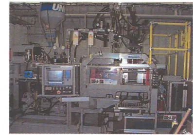
Figure 2. 5. Reciprocating­Screw Extrusion Blow Molding Machine Uniloy 250 Rl.

The extrusion blow molding process involves three consecutive stages:

The shape of the parison and its thickness distribution at the moment the mold closes are of central

importance (Dealy et. al., 1990). Diameter and thickness of the parison are not easily controllable because

of the flow rate variation during parison formation and the presence of gravitational forces (Tadmor Z.,

1979).

Factors governing the geometry of the parison include the die design, the resin properties and the

extrusion conditions (see Figure 2. 6). With regard to the resin, it is the rheological properties of the melt

that govern the parison shape, and it is highly desirable to be able to relate parison behavior to laboratory

rheological measurements.

Process conditions

Temperature  ^ \ < ^  ^i m e 

Extrusion rate ^ 

Die geometry

Types of  angles 

Converging Diverging 

Parison Formation ^ ( Diameter and thickness

distribution

Swell phenomena Sag phenomena

Figure 2. 6. Variables affecting diameter and thickness distribution of the parison shape.

The dynamics of the development of the parison are basically influenced by the swell and sag or

drawdown phenomena. The die swell phenomenon is also known as Barus effect, memory, jet swell, puff­

up, etc., and is to b e considered a manifestation of melt elasticity in a shearing flow through a die, where

the extrudate cross section (De) is greater than the cross section of the die diameter (D), that is De/D » 1 ,

(Koopmans 1988).

The variables usually employed to describe die swell are the swell ratio (B), the fully developed wall

shear rate (y w) , the length to diameter (L/D), the temperature (T), and the time (t) that has passed since

the melt left the die (Dealy et al. 1990).

Sag, or "draw­down", is caused b y gravitational forces that act on the suspended parison. The degree of

sag depends on processing parameters (such as melt temperature, suspension time and total parison length),

DiRaddo e t a l . (1992).

Nakajima N . (1974) established an empirical model to predict die swell. However this model did not

take in consideration material parameters, such as molecular weights, degree of branching, etc., and the die

geometry. H e stated that H D P E resins presented numerous variations for such model to be used in those

Guillet et al. (1965) and Combs et al. (1969) reported that die swell increases as the molecular weight

distribution broadens. These authors also found that the flow index "n" in the power law model decreases

as the molecular weight distribution broadens.

Kamal et al. (1981) calculated the diameter swell distribution using a time­dependent equation, and the

calculation agreed with the experimental data, but it was for short extrusion times (2 seconds). Also, Dealy

et al. (1985) found it to b e unrealistic and unreliable. Dealy argued that the model ignored the detailed role

played b y the strain history.

Kamal et al. (1981) used the following time­dependent equations:

Bi(t) was defined as: B](t) = Diameter of extrudate/Diameter of die

( A v + A , , ) '

  A v 

where  D O E = outside diameter of the extruded parison,  DI E = inside diameter of the extrudate parison,

DOD = outside diameter of the annular die, and  DID = inside diameter of the annular die.

B2(t) was defined as:B2(t) = Thickness of the parison, H/Thickness of the annular die,G.

m

  K

. ­ A , . ) / 2

g 

( 0

­ A v ) / 2 G 

The total length of the parison Ls (t) was given by:

£ f

( 0 = ' S A 4 ( 0

( 2 . 3 )

where N w a s the total number of increments extruded in time t, and

 AL's(t)was

element.

Dealy et al. (1985) found that 60­80% of the swell for commercial H D P E resins occurs in the first few

seconds after the parison leaves the die, with an equilibrium value being reached after 5­8 minutes have

elapsed. They saw that the die swell increased as the die shape (mandrel configuration) was altered in the

following order: diverging, straight, converging.

Koopmans, R. J. (1988) established an empirical relation between capillary die swell and molecular

structure defined b y total weight average weight (Mw T) , molecular weight distribution ( M W D ) , and

fraction high molecular weight content (FRB). The measurements of the die swell were conducted using an

Instron Rheometer with an L/D = 5.25 (D=0.531xl0"2_{m), at 300s'}1 _{and 190°C. A statistical analysis system}

(SAS) program w a s used to generate the interdependence of the 3 independent parameters in relation to

percentage swell (Mw A , MwB, and FRB). The empirical equation was modeled via statistical analysis of

the Box­Behnken experimental design:

Model =Y= K + aX{+bX2 + cX3 + dx\ + eX\

+

 fx] + gXxX2 + hX{X2 + iX2X3

(2. 4)