CARLOS MUNUERA AND WANDERSON TEN ´ORIO
Abstract. We give a method to construct Locally Recoverable Error-Correcting codes. This method is based on the use of rational maps between affine spaces. The recovery of erasures is carried out by Lagrangian interpolation in general and simply by one addition in some good cases.
1. Introduction
Error-Correcting codes are used to detect and correct any errors occurred during the transmission of information. A linear code of length n over the finite field Fq is just a
linear subspace C of Fn
q. If C has dimension k and minimum Hamming distance d we say that it is a [n, k, d] code.
Locally Recoverable (LRC) Error-Correctingcodes were introduced in [6] motivated by the recent and significant use of coding techniques applied to distributed and cloud storage systems. Roughly speaking, local recovery techniques enable us to repair lost encoded data by a ”local procedure”, which means by making use of small amount of data instead of all information contained in a codeword.
Let C be a [n, k, d] code over Fq. As a notation, given a vector x ∈ Fn
q and a subset
R ⊆ {1, . . . , n}, we write xR = prR(x) and CR = prR(C), where prR is the projection on the coordinates of R. A coordinate i ∈ {1, . . . , n} is locally recoverable with locality r if there is a recovering set R(i) ⊆ {1, . . . , n} with i 6∈ R(i) and #R(i) = r, such that for any codeword x∈ C, an erasure in position i can be recovered by using the information of xR(i). That is to say, if for all x,y ∈ C, xR(i) =yR(i) implies xi =yi. The code C has
all-symbol locality r if any coordinate is locally recoverable with locality at most r. We use the notation ([n, k], r) to refer to the parameters of such a code C.
The notion of local recoverability can be extended in two directions as follows: Firstly it can be desirable to dispose of codes with multiple recovering sets for each coordinate [15]. The codeC is said to havet recovering sets if for each coordinateithere exist disjoint sets
R(i, j), j = 1, . . . , t, such that #R(i, j)≤rj and the coordinatexi can be recovered from the coordinates of prR(i,j)(x) for all x∈ C, as above. The existence of several recovering sets is known as the availabilityproblem, as these codes make the recovering of loss data
2010Mathematics Subject Classification. 94B27, 11G20, 11T71, 14G50, 94B05.
Key words and phrases. error-correcting code, locally recoverable code, algebraic geometry code, Reed-Muller code, toric code.
better available. Secondly we can recover more than one erasure at the same time. C is said to have the (ρ, r) locality property if for each coordinate i there is a subset ¯R(i) containing i such that # ¯R(i) ≤ r+ρ−1 and ρ−1 erasures in xR¯(i) can be recovered
from the remaining coordinates of xR¯(i).
It is clear that every code of minimum distance d > 1 is in fact an LRC code able to recover ρ = d−1 erasures, simply by taking ¯R(i) = {1,2, . . . , n}. But such recovering sets do not fit into the philosophy of local recovery. We are interested in codes C allowing smaller recovering sets (in relation to the other parameters of C). In this sense, we have the following Singleton-like bound: the locality r of an [n, k, d] code C obeys the relation (see [6])
(1)
k r
≤n−k−d+ 2.
Codes reaching equality are called Singleton-optimal (or simply optimal) LRC codes, since they have the best possible relationship between these parameters. The number
n−k−d+ 2− ⌈k/r⌉ is the optimal defect of C. Similarly we say that C is Singleton-almost-optimal if, according to Eq. (1), no codes of type ([n, k+ 1, d], r) may exist, that is if (k+ 1)/r > n−(k+ 1)−d+ 2.
Slight modifications in the proof of Eq. (1) show that more generally, fort= 1, . . . , k, we have
k−t+ 1
r
≤n−k−dt+t+ 1
where d1, . . . , dk is the weight hierarchy ofC. We deduce r ≤ k and, from the duality of the weight hierarchy, r≥d⊥−1.
MDS codes (and Reed-Solomon codes in particular) satisfy CR = Fkq for every set R of
k positions, hence they have the largest possible locality r = k. Also, adding a parity check to k information symbols we get a ([(k+ 1)t, kt,2], k) optimal code for all positive integer t (which is MDS for t = 1). Optimal codes that either are MDS or have the previous parameters will be called trivial. The search for long nontrivial optimal codes is a challenging problem, and in fact for most known optimal nontrivial codes, the cardinality of the ground field Fq is much larger than the code length n, [16].
In [18] a variation of Reed-Solomon codes for local recoverability purposes was introduced by Tamo and Barg. These so-called LRC RS codes are optimal and can have much smaller locality than RS codes themselves. Its length is still smaller to the size ofFq. A classical
way to obtain larger codes is to use algebraic curves with many rational points. In this way LRC RS codes were extended by Barg, Tamo and Vladut [2, 3], to the so-called LRC Algebraic Geometry (LRC AG) codes, actually obtaining larger LRC codes.
V of functions such that any f ∈ V behaves as a univariate polynomial over each fibre of φ. Under appropriate conditions it is possible to recover such polynomials by using Lagrangian interpolation. Then the code ev(V), where ev is an evaluation map, is an LRC code whose recovering sets are the fibres ofφ.
The paper is organized as follows. The general construction of our codes is developed in Section 2. In the following two sections this construction is applied to some particular cases: to algebraic curves in Section 3 and to other geometric sets in Section 4. Each case is illustrated with several examples.
2. LRC codes from rational maps
The construction of LRC codes we propose relies on rational maps between affine spaces, extending ideas of [2, 18]. For the convenience of the reader, we begin by briefly recalling those constructions.
2.1. LRC codes from Algebraic Geometry. The construction of LRC RS codes is as follows [18]: let A(Fq) be the affine line over Fq and let P1, . . . ,Pt ⊂ A(Fq) be t > 1 pairwise
disjoint subsets of cardinality r + 1 such that there exists a polynomial φ(x) ∈ Fq[x]
of degree r + 1 which is constant over each Pi = {Pi,1, . . . , Pi,r+1}, i = 1, ..., t. Set
P =P1 ∪ · · · ∪ Pt and n =t(r+ 1). Fix an integer k such that r|k and k+ kr ≤n, and consider the linear space of polynomials
V =
r−1
X
i=0 k/r−1
X
j=0
aijφ(x)jxi : aij ∈Fq
.
The code C is obtained by evaluation of V at the points of P, evP : V → Fn
q, evP(f) = (f(Pij), i = 1, . . . , t, j = 1, . . . , r+ 1). Since deg(f) ≤ k+ kr −2 < n for all f ∈ V, the map evP is injective hence dim(C) = dim(V) = k. Furthermore given f ∈ V, for all
i= 1, . . . , t, there exists a polynomial fi(x) of degree ≤r−1 such thatfi(Pij) =f(Pij),
j = 1, . . . , r+ 1. Such fi’s can be computed through interpolation at any r points of Pi, so a recovering set for the coordinate corresponding to a point Pij is R(i) = Pi \ {Pij}. Then C is a linear ([n, k], r) LRC optimal code.
The above method is extended to construct LRC AG codes as follows [2, 3]: let X,Y be two algebraic curves over Fq and let φ : X → Y be a rational separable morphism of
degree r+ 1. Take a set S ⊆ Y(Fq) of rational points with totally split fibres and let
P =φ−1(S). Let D be a rational divisor on Y with support disjoint from S and denote
by L(D) its associated Riemann-Roch space of dimension m=ℓ(D). By the separability of φ there exists y∈Fq(X) satisfying Fq(X) =Fq(Y)(y). Let
V =
(r−1 X
i=0 m X
j=1
where{f1, . . . , fm}is a basis ofL(D). The LRC AG codeC is defined asC = evP(V)⊆Fnq, with n = #P. Note that C is a subcode of the algebraic geometry code C(P, G) = evP(L(G)), where G is any divisor on X satisfying V ⊆ L(G). In particular d(C) ≥
d(C(P, G))≥n−deg(G). Let evP(f),f ∈V, be a codeword in C. Since the functions of L(D) are constant on each fibreφ−1(S),S ∈ S, the local recovery of an erased coordinate
f(P) of evP(f) can be performed by Lagrangian interpolation at the remaining r coor-dinates of evP(f) corresponding to points in the fibre φ−1(φ(P)) of P. LRC AG codes
with availability have been studied in [9]. For a complete reference on algebraic geometry codes, see [10].
Theorem 1. [3, Thm. 3.1] If evP is injective on V then C ⊆ Fnq is a linear ([n, k, d], r)
LRC code with parameters n = s(r+ 1), k = rℓ(D) and d ≥ n−deg(D)(r+ 1)−(r− 1) deg(y).
Example 1. (Example 1 of [18]). The polynomial φ(x) = x3 ∈ F
13[x] is constant over
the sets P1 ={1,3,9}, P2 ={2,6,5} and P3 ={4,10,12}. By the first construction we
get optimal LRC codes of length 9, locality 2 and dimensions k= 2,4,6. The same codes can be obtained by the second construction from the curve X :x3 =y and the morphism
φ=y:X →P1.
Example 2. (a) Codes from the Hermitian curveH:xq+1 =y+yq over F
q2 were studied
in [3]. Consider the morphism φ = x : H → P1 of degree q. Take S = A(Fq2) ⊆ P1
and thus φ−1(S) =H(F
q2)\{Q}, where Q is the point at infinity of H. If D =l∞ then
V =Lr−1
i=0h1, x, x2, . . . , xliyi⊆Fq2(H). We get codes of localityr=q−1 and parameters
n=q3,k =r(l+ 1), d≥n−deg(G), whereG= (−v
Q(xlyr−1))Q and vQ is the valuation atQ.
(b) Codes from the Norm-Trace curve x1+q+···+qu−1
= y+yq+· · ·+yqu−1
over Fqu were studied by Ballico and Marcolla in [1]. Following similar ideas they found a family of LRC codes of locality r =qu−1−1, length n =q2u−1 and dimension k = (t+ 1)(qu−1−1).
2.2. LRC codes from rational maps. Let φ1, . . . , φt, φt+1 ∈ Fq(x1, . . . , xm) be rational functions and let A ⊆ Am(Fq) be a subset in which none of these functions have poles.
Then the map φ = (φ1, . . . , φt) : A ⊆ Am(Fq) → At(Fq) is well defined. Take two sets S ⊆At(Fq) and P ⊆φ−1(S) and define r= minS∈S∗#{φt+1(P) :P ∈ P, φ(P) =S} −1,
where S∗ =
{S ∈ S : φ−1(S)6=∅}. Thus, the function φ
t+1 takes at least r+ 1 different
values in the points of the fibre φ−1(S) for all S ∈ S∗. If r > 0, for i = 0, . . . , r −1, consider a linear Fq-spaceVi ⊂Fq[φ1, . . . , φt], and let
(2) V =
r−1
M
i=0
Viφit+1 ⊂Fq[φ1, . . . , φt+1]⊂Fq(x1, . . . , xm).
We define the code C =C(P, V) as the image of the evaluation at P map evP :V →Fn
dim(V). FurthermoreC is an LRC code of localityr, where recovering is obtained through Lagrangian interpolation in each fibre of φ: let f ∈V and suppose we want to recover an erasure at position f(P). Let S =φ(P) and {P1, . . . , Pr+1 =P} ⊆ φ−1(S)∩ P a set in
whichφt+1takesr+1 different values. Since all functions in eachViare constant in the fibre ofS, the restriction off to this fibre can be written as a polynomialfS =Pjr−=01ajTj, that isf(Pj) =fS(φt+1(Pj)) for allj = 1, . . . ,#φ−1(S). Sinceφt+1 takes at leastr+ 1 different
values in φ−1(S), the polynomialf
S may be computed by Lagrangian interpolation from
φt+1(P1), . . . , φt+1(Pr).
Example 3. Consider the rational functions φ1 =x/y, φ2 = (y−1)/z and the map φ =
φ1 : A ⊂ A3(F3) → A1(F3), where A = {(x, y, z) ∈ A1(F3) : yz = 06 }. Let S = A1(F3).
Then φ−1(0) = {(0,1,1),(0,1,2),(0,2,1),(0,2,2)}, φ−1(1) = {(1,1,1),(1,1,2),(2,2,1),
(2,2,2)},φ−1(2) ={(1,2,1),(1,2,2), (2,1,1),(2,1,2)}. Note thatφ
2(0,1,1) =φ2(0,1,2);
φ2(1,1,1) = φ2(1,1,2) and φ2(2,1,1) = φ2(2,1,2). We set P = {(0,1,2),(0,2,1),
(0,2,2); (1,1,2), (2,2,1),(2,2,2); (1,2,1),(1,2,2),(2,1,2)}and hence r = 2. If we take the spaces of functions
V1 =h1,
x
yi ⊕ h1i y−1
z and V2 =h1, x y,
x2
y2i ⊕ h1,
x yi
y−1
z
we get a ([9,3,6],2) optimal LRC code C1 (from V1) and a ([9,5,3],2) optimal code C2
(from V2). Both have length much larger than the cardinality of F3. In fact, the length
and locality of these codes are the same as those of Example 1, although the cardinal of the ground field is considerably smaller.
Defined in such generality, it is not possible to say too much about the parameters and be-haviour of codes obtained by the aforementioned construction. In the subsequent sections we will discuss in more detail several particular classes of codes given by this method. As we shall see, in some of these cases the local recovery can be done by a simple checksum and does not require interpolation, which is simpler and faster.
Example 4. For both codes C1 and C2 of Example 3, a direct inspection shows that
for any codeword evP(f),f ∈V2 (as defined in Example 3), the sum of their coordinates
corresponding to each fibre ofφis zero. Thus a single erasure is corrected by one addition. This construction also allows us to recover more than one erasure. Following the standard notation as in the Introduction, suppose we want to correct ρ−1 erasures in the coordi-nates corresponding to a fibre ofφ. For this, let r= minS∈S∗#{φt+1(P) :P ∈ P, φ(P) =
S} −ρ, consider the space of functions V as stated in equation (2), with respect to the new value of r, and define C = evP(V). The restriction of f ∈V to the points in a fibre of φ is a polynomial of degree r−1. It can be computed from the information of any r
3. LRC codes from Algebraic Curves 3.1. The construction for algebraic curves. Let X ⊂ Pm(F
q) be a (algebraic, projec-tive, absolutely irreducible) curve over Fq. Take a rational point Q ∈ X(Fq).
Af-ter a change of coordinates, if necessary, we can assume that Q is a point at infin-ity. The set L(∞Q) = ∪s≥0L(sQ) is a finitely generated Fq-algebra. Take rational functions φ1, . . . , φt+1 ∈ L(∞Q) and fix representatives of these functions (still denoted
φ1, . . . , φt, φt+1 by abuse of notation). Let A ⊆ X(Fq) be the set of rational affine points on X and consider the map φ = (φ1, . . . , φt) : A ⊆ Am(Fq) → At(Fq). Let S ⊆ At(Fq), P ⊆φ−1(S) andras in the general construction. For i= 0, . . . , r−1, fix linear F
q-spaces
Vi ⊂Fq[φ1, . . . , φt] and
V =
r−1
M
i=0
Viφit+1 ⊂Fq[φ1, . . . , φt+1].
Since φt+1 ∈ L(∞Q), no point of P is a pole of φt+1. We define the code C = C(P, V)
as the image of the evaluation at P map evP :V → Fn
q, where n = #P is the length of C. Note that the number of zeros of a function f is related to the value vQ(f), where vQ is the valuation atQ: the larger this number, then the smaller the weight of evP(f) may be. This fact leads us to use the language of polytopes to define the space of functions
V. For our purposes a polytope will be a set P ⊂ Nt+1
0 , where N0 stands for the set of
nonnegative integers. Often we shall takePas the convex hull of a set of points including (0, . . . ,0) and (0, . . . ,0, r−1).
Given a polytope Pwe can consider the associated linearFq-space V(P)⊆Fq[φ1, . . . , φt]
spanned by the functions {φα1 1 · · ·φ
αt+1
t+1 : (α1, . . . , αt+1) ∈ P}. In our case, for i =
1, . . . , t+ 1, let vi =−vQ(φi). For l≥1 we consider the polytope in Nt0+1
P=P(l) ={(α1, . . . , αt+1)∈Nt0+1 : v1α1+· · ·+vt+1αt+1 ≤l, αt+1 ≤r−1}.
If V = V(P(l)), then V ⊆ L(lQ) and hence C(P, V) is a subcode of the usual AG code
C(P, lQ). Then C(P, V) is an LRC code of localityr. When l < n= #P the evaluation map evP :L(lQ)→Fn
q is injective, then so is evP :V →Fnq, and the dimension ofC(P, V) is #P. The minimum distance of C(P, V) is at least the minimum distance of C(P, lQ), that is n−l.
Remark 1. Our construction of LRC codes from curves extends that given in [2, 3]. The main difference is in the set V of functions to be evaluated. In the language of [2, 3], rather than considering a unique divisor D, we may consider r rational divisors
D0, . . . , Dr−1 onY, the space of functions V =Lir=0−1L(Di)yi and the code evP(V)⊆Fnq. This change does not affect the locality nor the recovering method. Using a sequence of divisors D0, . . . , Dr−1, instead of a single divisor D provides greater flexibility to the
construction. Typically one can take D0 ≥ · · · ≥ Dr−1. Since codewords of smaller
to increase the dimension of C without affecting the estimate on the minimum distance. In Subsection 3.4 we shall show several examples of this fact. Recall that codes of this type were already considered by Maharaj in [13] using the language of function fields. In that paper, it is shown that the smallest divisor G satisfying V ⊆ L(G) is described as
G= max{(φ∗(D
i)−div(yi) : 0≤i≤r−1}, whereφ∗ : Div(Y)→Div(X) is the pull-back map induced by φ.
In the rest of this section we present examples of LRC codes obtained from some types of curves which are well known in coding theory.
3.2. LRC codes from the Klein quartic. The Klein quartic is the curveK defined overF8
by the affine equation x3y +y3+x = 0. Codes from this curve have been extensively
studied, [8]. It has 24 rational points, being two of them at infinity, R = (0 : 1 : 0) and
Q= (1 : 0 : 0). The Weierstrass semigroups at R and Q are both equal toh3,5,7i. The rational functions φ1 =x/y and φ2 =x/y2 have poles only at Q, with multiplicity 3 and
5 respectively.
Example 5. Let A be the set of affine rational points of K and consider the rational function φ1 : A → A1(F8). The only ramified point of φ1 is (0,0), hence #φ−11(S) = 3
for all S ∈ A1(F8), S 6= 0. Take S = A1(F8)\ {0} and P = φ−1
1 (S) = A \ {(0,0)}.
Since φ2 takes 3 distinct values in all fibres φ−11(S),S ∈ S, we have r= 2. The polytope P = P(6) = {(α, β) ∈ N2
0 : 3α+ 5β ≤ 6, β ≤ 1} leads to the space of functions
V = h1, φ1, φ21i ⊕ h1iφ2 which, through evaluation at P, produces a ([21,4,15],2) LRC
code of optimal defect 2. Let us note that according to the Griesmer bound, the maximum possible minimum distance d for a linear [21,4]8 code is d = 16, and therefore optimal
([21,4]8,2) LRC codes cannot exist.
In the same way, by considering polytopes P(l), 1 ≤ l ≤ 20, we obtain LRC [n, k] codes, 1 ≤ k ≤ 13, of locality 2. Those of dimension 1,11,13 are optimal. For the rest, those of odd dimension have defect 1 and those of even dimension have defect 2. The true minimum distances of these codes have been computed with the computer system Magma [12]. In the non-optimal cases, further modifications of the above polytopes can lead to codes with better parameters. For example, if we remove (6,0) from P(20), we get a [21,12,4] almost-optimal code. The same happens for the other values of l.
3.3. LRC codes from elliptic curves. Let X be an elliptic curve over Fq. If we assume
char(Fq) = p 6= 2,3, then X has a plane model given by an affine equation of the form y2 =x3+ax+b and exactly one point at infinity,Q. Although the above theory may be
applied to any elliptic curve, in this section, by way of example, we shall restrict ourselves to those of equations y2 =x3+B. Ifq ≡3 (mod 3) then all of them have q+ 1 rational
Assumeq ≡1 (mod 3) and letξ be a primitive element ofFq. Since ω=ξ(q−1)/3 is a cubic
root of unity, for each of these curves X, if (a, b) ∈ X(Fq) then also (ωa,±b) ∈ X(Fq).
Thus the set A of rational affine points (a, b) of X with a 6= 0 can be grouped in triples, {(a, b),(ωa, b),(ω2a, b)}, and a= 0 happens at most for two points. We can obtain LRC
codes of locality r= 2 from X. To this end, letA be the set of points belonging to these triples,φ =y :A ⊂ A2 →A1,S =A1andP =A ⊆φ−1(A1). Letn= #P ≥#X(Fq)−3.
Since −vQ(x) = 2,−vQ(y) = 3, for l ≥1 we consider the polytope P(l) ={(α, β)∈N20 :
2α+3β ≤l, α≤1}of cardinality #P(l) =l−⌊(l−1)/3⌋and the linear space of functions
V(l) = h{xαyβ : (α, β) ∈ P(l)}i ⊂ L(lQ). Let C = C(P, V(l)) obtained by evaluation at P of all functions in V(l). SinceC(P, V(l)) ⊆C(P, lQ), if l < n then evP is injective, so the dimension of C is #P(l) and its minimum distance is n−l. A straightforward computation shows that having these parameters, C is optimal when l ≡ 0 (mod 3) and almost-optimal when l≡2 (mod 3).
In order to determine the length of these codes, we shall study the number of rational points on our curves. There exist six isomorphism classes of such curves, namelyXi :y2 =
x3+ξi, i = 0, . . . ,5. In [14] a fast algorithm to determine the cardinality of all of them can be found. However, we do not use this algorithm here and we will limit ourselves to using some elementary facts established in that article. Write Si = #Xi −q−1. Since X0 ∼= X3, X0 ∼= X3, X0 ∼= X3 over Fq2, X0 ∼= X2 ∼= X4, X1 ∼= X3 ∼= X5 over Fq3, and all
of them are isomorphic over Fq6, we deduce that S0 = −S3, S1 = −S4, S2 = −S5 and
S2
0 +S12 +S22 = 6q. Then any of these six curves Xi has at least q+ 1 +√2q points. If
q is an even power, then any of these six curves Xi has q+ 1 + 2√q points. Even in the case that q is an odd power, numerical experiments show that in most cases any of these six curves has either q+ 1 + 2√q or q+ 2√q points. In conclusion, when q ≡ 1 (mod 3) we can always find optimal LRC codes of locality r= 2 and length n ≥q+√2q−2. Example 6. Consider the field F13and the primitive element ξ= 2. The curve X2 :y2 = x3 + 4 has 20 affine points (the maximum possible), namely (7,±3),(8,±3),(11,±3);
(4,±4),(10,±4),(12,±4); (2,±5),(5,±5),(6,±5) and (0,±2). We obtain LRC Elliptic codes of length n = 18, locality r = 2 and dimensions k = 1, . . . ,12. Those of odd dimension are optimal whereas those of even dimension are almost-optimal. Remark that the length of these codes is twice the length of those of Example 1.
3.4. LRC codes from Hermitian curves. Among all curves used to obtain AG codes, Her-mitian curves H:xq+1 =yq+y over F
q2, are by far the most studied and best known. In
Example 7. Consider the Hermitian codeC treated in [3, Section IV] and Example 2(a). It is constructed overFq2 as the evaluation codeC = evP(V) from the Hermitian curveH,
the setP =H(Fq2)\ {Q}, whereQis the only point at infinity, and the space of functions
V =Lr−1
i=0h1, x, x2, . . . , xliyi. Thenr =q−1. C can be obtained also from the rectangular
polytope P = {(α, β) ∈ N2
0 : α ≤ l, β ≤ r−1}. In order to compare this code with
some others obtained through our construction of Section 3.1, we note that −vQ(x) =
q,−vQ(y) =q+ 1 and so max{−vQ(f) : f ∈V}=lq+ (r−1)(q+ 1). This fact suggests to consider the polytopeP′ ={(α, β)∈N2
0 : qα+(q+1)β ≤lq+(r−1)(q+1), β ≤r−1}
which leads to the space of functionsV′ =Lr−1
i=0h1, x, x2, . . . , xliiyi withli =l+r−i−1,
i= 0, . . . , r−1, and the code C′ = evP(V′). Note that V, V′
⊆ L((lq+ (r−1)(q+ 1))Q), hence whenever lq+ (r−1)(q+ 1)< n=q3, both maps evP :V →Fn
q and evP :V′ →Fnq are injective. So dim(C) = (l+ 1)r and dim(C′) = #P = dim(
C) + ((r−1) +· · ·+ 0). Thus there is a gain of (r−1) +· · ·+ 1 = (q−1)(q−2)/2 units in the dimension of C′ without affecting the estimate on the minimum distance. For example, if q = 5 then for any value of l ≤ 21, evP is injective, the dimension increases by 6 units and the optimal defect decreases by 8 units.
Example 8. Consider again the Hermitian code C of Example 2(a). Let us take here the opposite way to the previous Example 7 and construct LRC Hermitian codes with improved minimum distance and at least the same dimension. Let V and C as in Ex-ample 7. Let l′ = l − ⌊r(r − 1)/2q⌋. Consider now the space of functions V′ = Lr−1
i=0h1, x, x2, . . . , xl
′
iiyiwithl′
i =l′+r−i−1,i= 0, . . . , r−1, and the codeC′ = evP(V′). Note that l′ = l − ⌊r(r−1)/2q⌋ implies q(l′ + 1) + r(r −1)/2 ≥ q(l + 1) so, accord-ing to the considerations made in Example 7, dim(C′)
≥ dim(C). Furthermore, since
V ⊆ L((lq + (r− 1)(q + 1))Q), V′
⊆ L((l′q+ (r
−1)(q + 1))Q), the estimate on the minimum distance of C′ is (l −l′)q ≈ r(r−1)/2 units larger than the estimate on the minimum distance of C. For example, if q = 5 then dim(C) = 5l+ 5, dim(C′) = 5l+ 6 and the estimate on the minimum distance of C′ is 5 units larger than the estimate on the minimum distance of C. Numerical experiments using Magma to compute the true minimum distances of these codes show that this is the case for most values of l.
3.5. AG Hermitian codes as LRC codes. LetC = evP(V) be an LRC code obtained from a curve X, a point Q and the sets P and V. Our estimate on the minimum distance of C comes from the Goppa bound on the minimum distance of the smallest AG code
f ∈Fq2[x][y] with degy(f)< q. Such f may appear in the set V of an LRC code arising
fromH if degy(f)< q−1.
Proposition 1. Let H be the Hermitian curve over Fq2. The space of functions V =
Lt
i=0h1, x, x2, . . . , xliiyi ⊆Fq2(H), with t ≤ q−2, is a Riemann-Roch space L(G) if and only if there existsj, 0≤j ≤t+ 1, such that lt−i =i if i < j and lt−i =i+ 1if i≥j. In
this case G=sQ, where Q is the point at infinity of H and s= (t+ 1)q+t−j if j ≤t or s=t(q+ 1) if j =t+ 1.
Proof. The smallest Riemann-Roch space containingV isL(sQ) withs= max{−vQ(xliyi) :
i = 0, . . . , t} = max{liq+i(q+ 1) : i= 0, . . . , t}. Let us first assume V =L(sQ). Then for i = 0, . . . , t, we have lt−i ≤ i+ 1, since otherwise −vq(xlt−iyt−i) > −vQ(xi+2yt−i) > −vQ(yt+1) so yt+1 ∈ V. In particular lt = 0 or lt = 1. A similar argument proves that for all i = 1, . . . , t, we have li−1 ≥ li + 1. From these two conditions we deduce that there exists j, 0 ≤ j ≤ t+ 1, such that lt−i = i if i < j and lt−i = i+ 1 if i ≥ j. Con-versely, it is simple to check that under these conditions we have s = −vQ(xlt−jyt−j) = (j+ 1)q+ (t−j)(q+ 1) = (t+ 1)q+t−j ifj ≤tand s=−vQ(yt) =t(q+ 1) ifj =t+ 1. In either case it holds that dim(V) =ℓ(sQ), hence we get equality V =L(sQ). Example 9. Consider the LRC codes obtained from the Hermitian curve with q= 4 and the map φ = x. For short let us restrict to those codes correcting one erasure per fibre (t= 2). There are exactly four among them which are AG codes, namely the evaluation of the following spaces
V =h1, x, x2i ⊕ h1, xiy⊕ h1iy2 =L(−vQ(y2)Q) = L(10Q)
V =h1, x, x2, x3i ⊕ h1, xiy⊕ h1iy2 =L(−vQ(x3)Q) =L(12Q)
V =h1, x, x2, x3i ⊕ h1, x, x2iy⊕ h1iy2 =L(−vQ(x2y)Q) =L(13Q)
V =h1, x, x2, x3i ⊕ h1, x, x2iy⊕ h1, xiy2 =L(−vQ(xy2)Q) =L(14Q).
3.6. A simplified recovering method for LRC Hermitian and related codes. In order to motivate this subsection, we begin with a simple example.
Example 10. Let us consider the LRC Hermitian code C = evP(V) constructed over
F9 from the Hermitian curve H, the map φ = x, the set P = H(F9)\ {Q} where Q is
the only point at infinity of H, and the space of functions V =Lr−1
i=0h1, x, x2, . . . , xliiyi,
wherer =q−1 = 2. Each fibreφ−1(a) is of type{(a, b
1),(a, b2),(a, b3)} witha4 =b3i +bi for i = 1,2,3. Since a function f ∈ V can be written as f = g0(x) +g1(x)y, we have
f(a, bi) =g0(a) +g1(a)bi and thus
f(a, b1) +f(a, b2) +f(a, b3) = 3g0(a) +g1(a)(b1 +b2+b3) =g1(a)(b1+b2+b3) = 0
because b1+b2 +b3 = 0 as it is the sum of the roots of the polynomial y3+y−a4 (the
coefficient of y2). Then the coordinate f(a, b
1) of the codeword evP(f) can be recovered
In this subsection we shall show a family of LRC codes from curves with this prop-erty of recovering by checksum. We first recall some identities regarding roots of uni-variate polynomials. Consider the elementary symmetric polynomials over a domain A,
σ1(z1, . . . , zd) =z1+· · ·+zd, σ2(z1, . . . , zd) =z1z2+· · ·+zd−1zd, . . . , σd(z1, ..., zd) =z1· · ·zd. Writeσi =σi(z1, ..., zd). For an arbitrary monic polynomialt(x) =xd+td−1xd−1+· · ·+t0 ∈
A[x], the elementary symmetric polynomials on the roots z1, ..., zd of t(x) are related to its coefficients by the Vieta’s formulae [4]: σi = (−1)itd−i, i = 1, ..., d. Consider now for
i≥1 the multivariate polynomials πi =πi(z1, ..., zd) =z1i +· · ·+zid∈A[z1, . . . , zd],which are related to the elementary symmetric polynomials by the Newton-Girard relations [4]: we have π1 =σ1 and for each integer i >1,
πi = (−1)i−1iσi− i−1
X
j=1
(−1)jπi−jσj.
Letpbe the characteristic ofFq. Recall that a polynomialℓ(x)∈Fq[x] is linearizedif the
exponents of all its nonzero monomials are powers of p. In that case, any polynomial of the form ℓ(x)−α, α∈Fq, will be calledaffine p-polynomial.
Lemma 1. If z1, ..., zd are the roots of an affine p-polynomial of degree d over Fq, then
πi(z1, ..., zd) = 0 for all i= 1, . . . , d−2.
Proof. By induction. Clearly π1 = σ1 = 0. Assume π1 = · · · = πi−1 = 0 for i ≤ d−3.
Then πi =±iσi. If σi = 0 we have πi = 0. If σi 6= 0 then d−i= ph −i is a power of p. Thus i≡0 (mod p) and again πi = 0. Thereforeπ1 =. . .=πd−2 = 0.
Next we extend the idea of Example 10 to a wide class of curves providing families of LRC codes allowing local recovery by a checksum. The codes we propose come from the family of Artin-Schreier curves and thus they include LRC Hermitian codes. More precisely let X be an algebraic smooth curve defined over Fq by an equation of separated variables u(x) =v(y), where u and v are univariate polynomials over Fq of coprime degrees and v
is a separable linearized polynomial of degree m=ph, withp= char(F q).
X has exactly one point at infinity Q which is the common pole of x and y. The Weier-strass semigroup of X at Q is generated by −vQ(x) = deg(v) and −vQ(y) = deg(u). Consider the rational map φ = x : X(Fq) \ {Q} → A1 and let S = {a ∈ Fq :
there exists b ∈Fq with u(a) = v(b)}. By our assumptions on v, for each a ∈ S the
function x−a has m distinct zeroes and thus the fibre φ−1(a) consists of m points. Let
P =φ−1(S) and n= #P =m#S. For a positive integer l < nwe consider the polytope P = {(α, β) ∈ N2
0 : deg(v)α+ deg(u)β ≤ l, β ≤ m−2}, which leads to the space of
functions V =Lm−2
i=0 h1, x, . . . , xliiyi. Clearly it holds that V ⊆ L(lQ). Consider also the
set of points P =φ−1(S)\{Q}. Then we have a code C = evP(V) of length n, dimension
Proposition 2. The linear code C described above allows a local recovery based on one addition.
Proof. Letφ−1(a) ={P
1, ..., Pm}be the fibre ofa∈ Sand writefaj =f(Pj) the evaluation atPj ∈φ−1(a) off =Pim=0−2giyi∈V. The functionsgi are constant over each fibre so we can write gi =gi(Pj) ∈ Fq for any Pj ∈ φ−1(a). Then faj = g0b0j +· · ·+gm−2bmj −2 with
bj =y(Pj) and so m X
j=1
faj =mg0 +g1π1+· · ·+gm−2πm−2 =g1π1+· · ·+gm−2πm−2
where πi = πi(b1,· · · , bm) is the i-th Newton-Girard polynomial on the roots b1, . . . , bm of ℓ(y) =v(y)−u(a). Since ℓ(y) is an affine p-polynomial, it follows from Lemma 1 that
π1 =· · ·=πm−2 = 0. Therefore fa1+· · ·+fam = 0 and the recovery of an erased symbol
faj is obtained through addition of the remaining symbols in the fibre φ−1(a). Example 11. Hermitian and Norm-Trace curves, among many others, belong to the family of curves we have considered. Thus LRC codes arising from them admit recovering of single erasures by one addition.
4. LRC codes from other sets of points
The same ideas and methods of the previous section can be applied to different geometric objects, other than algebraic curves. In this section we will discuss three cases related to Affine Variety codes, Toric codes and Reed-Muller codes. All of them are well-known in Coding Theory.
4.1. Polytopes, polynomials and codes. Let us consider Fq[x1, . . . , xm] the ring of
poly-nomials in m indeterminates over the field Fq. A monomial in Fq[x1, . . . , xm] is called reduced if its degree in each variable is at most q−1. A polynomial is reduced if it is a linear combination of reduced monomials. For any polynomial f ∈ Fq[x1, . . . , xm] there
is a reduced polynomial f∗ (obtained by reducing mod q all exponents of f) such that
f(P) = f∗(P) for all P ∈ Am(F
q). Thus, in what follows we shall restrict to consider reduced polynomials.
Given a polytope P ⊆ [0, q − 1]m and two sets A ⊆ Am(F
q), S ⊆ At(Fq), we can construct codes in the usual way. Let φ : Am → At be the projection on t coordinates
and P = φ−1(S). We have the code C = C(P, V(P)). When these sets are properly
chosen then C is an LRC code. The most obvious choices for a polytope are simplices and hypercubes. Following the usual notation, given integers l, l1, . . . , lm, we write
Note that when P = ∆(l) and P = Am(F
q) we obtain the Reed-Muller code RM(l, m), [10]. Next we shall state some properties of codes C(P, V(P)).
Proposition 3. Let P ⊆ H(q, . . . , q) ⊆ Nm
0 be a polytope, P ⊆ Am(Fq) a subset with
n points and C = C(P, V(P)). Let l be the maximum degree of a polynomial in V(P). Write (q−1)m−l=θ(q−1) +µ with 0≤ µ < q−1 and set δ = (µ+ 1)qθ. Then
(a) the minimum distance of C is at least δ−qm+n; (b) if δ > qm−n then ev
P :V(P)→Fmq is injective so dim(C) = #P.
Proof. Sincelis the maximum degree of a polynomial inV(P), thenC ⊆RM(l, m), whose minimum distance is δ, [10]. Furthermore P is obtained from Am(Fq) by deleting qm−n
points. Both statements (a) and (b) are direct consequences of this fact. The following result was proved for the case of Toric codes in [17].
Proposition 4. Let m1, m2 be positive integers and m=m1m2. Consider the sets P1 ⊆
Am1(F
q), P2 ⊆ Am2(Fq), P = P1 × P2 ⊆ Am(Fq) and the polytopes P1 ⊆ [0, q−1]m1, P2 ⊆[0, q−1]m2, P=P1×P2 ⊆[0, q−1]m. LetV
1, V2, V be the linear spacesV1 =V(P1),
V2 =V(P2), V =V(P). If both maps evP1 :V1 →F m1
q and evP2 :V2 →F m2
q are injective,
then
(a) the map evP :V →Fmq in injective; and
(b) the minimum distances of the codesC(P1, V1), C(P2, V2),C(P, V), satisfyd(C(P, V)) =
d(C(P1, V1))·d(C(P, V)).
Proof. Writen1 =P1, n2 =P2, n=n1n2 =P andd1 =d(C(P1, V1)), d2 =d(C(P, V)), d=
d(C(P, V)). A polynomial f ∈V, f 6= 0, can be written as
f = X
β∈P2
fβ(x)yβ
whereβ = (β1, . . . , βm2), y
β =yβ1 1 . . . y
βm2
m2 and fβ ∈V1. Denote byZ(f) the set of zeroes
of f. (a) Since evP1 is injective, there exists a point P1 ∈ P1 such that f(P1,y) 6= 0.
Now since evP2 is injective, there exists a point P2 ∈ P2 such that f(P1, P2) 6= 0 and so
evP(f) 6= 0. (b) Let P1 ∈ P1. If P1 ∈ Z({fβ(x) : β ∈ supp(f)}) then f(P1,y) = 0
so #Z(f(P1,y)) = n2. Observe that in this case we have P1 ∈ Z(Pfβ(x))∩ P1. Since
P
fβ(x)∈V1 and evP1 is injective, this possibility happens for s ≤n1−d1 points P1. If
P1 6∈Z({fβ(x) : β∈supp(f)}) thenf(P1,y) has at most n2−d2 zeros P2 ∈ P2 because
evP2 is injective. Thus
#Z(f)≤sn2+ (n1−s)(n2−d2) = n−d2(n1−s)≤n−d1d2
so wt(f) ≥ d1d2 and d ≤ d1d2. Conversely if f1 ∈ V1, f2 ∈ V2 then f1f2 ∈ V and
Corollary 1. Let l1, . . . , lm ≤ q be positive integers and let P be the hypercube P = H(l1, . . . , lm). Let P =P1× · · · × Pm ⊆Am(Fq) with ni = #Pi ≥li for all i = 1, . . . , m.
Then evP : V(P) → Fmq in injective, so dim(C(P, V(P))) = #P and d(C(P, V(P))) = Q
i(ni−li + 1).
Proof. H(l1, . . . , lm) is the product of m segments [0, li −1], each of them leading to a Reed-Solomon code. The result follows from Proposition 4.
4.2. LRC codes from Affine Variety codes. Givenmpositive integersn1, . . . , nm, such that
ni|q−1 for all i, set vi = (q−1)/ni and consider the ideal I of Fq[x1, . . . , xm] generated by the monomials xn1
1 −1, . . . , xnmm −1. LetA be the set of zeroes of I,A =Z(I). Ifξ is a primitive element of Fq then ξvi is a root of xni
i −1, hence A consists of n =n1· · ·nm points. Furthermore, if we consider the projection map φ = (x1, . . . , xi−1, xi+1, . . . , xm) :
Am →Am−1, for every point S∈ S =φ(A) we have #φ−1(S) =ni.
For a polytope P ⊆ H(n1, . . . , nm) we consider the linear space of polynomials V(P) = h{xα1
1 · · ·xαmm : (α1, . . . , αm) ∈ P}i and define the Affine Variety code C as the image of the evaluation map, C =C(A, V(P)) = evA(V(P)). Then C is a code of length n and dimension #Pby Corollary 1. Note that in the language of Section 3, we take P =A. Now we intend to give some properties on P in order to obtain LRC codes whose local recovery is based on polynomial interpolation. Define the degree of P with respect to i
(or i-degree of P) to be the maximum i-degree of a polynomial in V(P).
Theorem 2. If P has i-degree r− 1 with 1 ≤ r ≤ ni −1 for some i, then the code C(P, V(P)) is a locally recoverable code of locality r. The local recovery of an erased symbolf(P), P ∈ P, may be performed by Lagrangian interpolation at any r other points in the fibre φ−1(φ(P)).
Proof. Note that the fibre φ−1(φ(P)) has n
i −1 points different from P. Write V =
V(P) = Lr−1 j=0Vj x
j
i, with Vj ⊂ Fq[x1, . . . , xi−1, xi+1, . . . , xm]. For f ∈ V(P) we can write f = P
gjxji with gj ∈ Vj. Observe that these gj’s are all constant in the fibre
φ−1(φ(P)) and thus f(P) can be recovered by interpolating a univariate polynomial in
the indeterminate xi.
The same approach provides locally recoverable codes for multiple errors and enables us to consider LRC codes with availability.
Corollary 2. IfP has i-degree ni−j for somei, j, with j ≥2, then the code C(P, V(P))
is a locally recoverable code for multiple errors, of locality r=ni−1 and capability ρ=j.
Corollary 3. If P has ij-degree r −1 for some i1, . . . , it, and 1 ≤ r ≤ nij −1, then
the code C(P, V(P)) is a locally recoverable code with t-availability and locality r for all i1, . . . , it.
The most obvious choice to produce LRC Affine Variety codes is to take i = m and the polytope P = H(n1, n2, . . . , nm−1), which gives a code C =C(P, V(P)) of locality
r = nm −1. ¿From Corollary 1, the minimum distance of C is 2 so it is an optimal trivial code. Subsequent manipulations of that polytope also provide interesting codes. Note that whenP is a hypercube inH(n1, n2, . . . , nm−1) then the minimum distance of C(P, V(P)) is also given by Corollary 1.
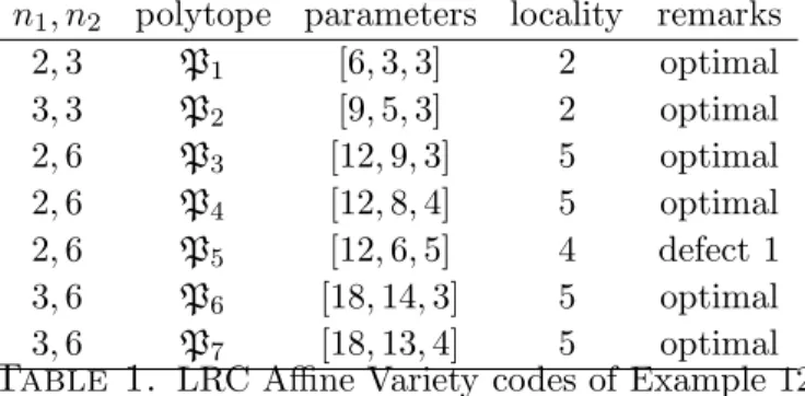
Example 12. Consider the fieldF7, the ring of polynomials in two variables F7[x, y] and
the projection φ =x:A2 →A1. Let us show some LRC codes obtained by the previous
construction. The following Table 1 contains the parameters of nontrivial LRC codes obtained by using the following polytopes: P1 =H(2,2)\{(1,1)},P2 =H(3,2)\{(2,1)}, P3 = H(2,5)\ {(1,4)}, P4 = P3 \ {(1,3)}, P5 = P4 \ {(1,2),(0,4)}, P6 = H(3,5)\
{(2,4)}, P7 =P6\ {(2,3)}. The minimum distances of these codes have been computed
with Magma. The codes corresponding to the polytopes P3,P4 have the best known
parameters according to the tables [7].
n1, n2 polytope parameters locality remarks 2,3 P1 [6,3,3] 2 optimal
3,3 P2 [9,5,3] 2 optimal
2,6 P3 [12,9,3] 5 optimal
2,6 P4 [12,8,4] 5 optimal
2,6 P5 [12,6,5] 4 defect 1
3,6 P6 [18,14,3] 5 optimal
3,6 P7 [18,13,4] 5 optimal
Table 1. LRC Affine Variety codes of Example 12
Example 13. Consider again the field F7, the ring of polynomials in three variables F7[x, y, z] and the projection φ = (x, y) : A3 → A2. The following Table 2 contains
the parameters of nontrivial LRC codes obtained by using the following polytopes: Q1 = H(2,2,2)\{(1,1,1)},Q2 =Q1\{(1,1,0)}Q3 =H(2,2,5)\{(1,1,4)},Q4 =Q3\{(1,1,3)}, Q5 = H(3,3,2)\ {(2,2,1)}, Q6 = Q5 \ {(2,2,0)}, Q7 = H(3,3,5)\ {(2,2,4)}, Q8 = Q7\ {(2,2,3)}.
4.3. LRC codes from Toric codes. Affine Variety codes with ni =q−1,i= 1, . . . , m, are called Toric codes. In this case n = (q−1)m and A =P = (F∗
q)n. Toric codes are rather well known and this family includes some codes with good parameters, [11].
n1, n2, n3 polytope parameters locality remarks
2,2,3 Q1 [12,7,3] 2 optimal
2,2,3 Q2 [12,6,4] 2 almost-optimal
2,2,6 Q3 [24,19,3] 5 optimal
2,2,6 Q4 [24,18,4] 5 optimal
3,3,3 Q5 [27,17,3] 2 optimal
3,3,3 Q6 [27,16,4] 2 almost-optimal
3,3,6 Q7 [54,44,3] 5 optimal
3,3,6 Q8 [54,13,4] 5 optimal
Table 2. LRC Affine Variety codes of Example 13
the simplex ∆(l), l ≤ q−1. Recall that #∆(l) = mm+l
and the minimum distance of C(P, V(∆(l))) is known to be (q−1)m−1(q−l−1), [11].
Example 14. Consider the field F7, the rings of polynomials in two and three variables
and the projection φ =x. The following Table 3 contains the parameters of LRC codes obtained by using the following polytopes: P1 = H(6,5)\ {(5,4)}, P2 = P1 \ {(5,3)}, P3 =P2\ {(5,2),(4,4)},P4 =P3\{(5,1)},R1 = ∆(4)\{(4,0),(0,4)} in dimension two; and Q1 = H(6,6,5)\ {(5,5,4)}, Q2 = Q1 \ {(0,0,0)} in dimension three. For a better
understanding of these results we recall that the best known [36,25] and [36,13] codes over F7 have minimum distances 7 and 17 respectively, [7].
polytope parameters locality remarks
P1 [36,29,3] 5 optimal
P2 [36,28,4] 5 optimal
P3 [36,26,5] 5 defect 1
P4 [36,25,6] 5 defect 2
R1 [36,13,15] 4 availability 2
corrects 2 erasures
Q1 [216,179,3] 5 optimal
Q2 [216,178,4] 5 optimal
Table 3. LRC Toric codes of Example 14
4.4. LRC codes from Reed-Muller codes. Let R[x1, . . . , xm] be the set of reduced poly-nomials in Fq[x1, . . . , xm] and R[x1, . . . , xm]l be the set of reduced polynomials of
to-tal degree at most l. Note that these sets are the spaces of functions V(P) associated to the polytopes P = H(q, . . . , q) and P = ∆(l), respectively. It is well known that the evaluation at A = Am(Fq) map evA : R → Fn
q is an isomorphism ([10] or Corol-lary 1). The Reed-Muller code RM(l, m) is defined as RM(l, m) = evA(R[x1, . . . , xm]l). When l ≤ q−2 this is already an LRC code. To see that we take S = Am−1(Fq), the
S ∈Am−1(F
q) the fibreφ−1(S) consists ofq points, hence RM(l, m) has localityr =q−1 and length n = #Am(F
q) =qm. When l ≤ q−1 then RM(l, m) has minimum distance
d= (q−l)qm−1 and dimension is #∆(l) = m+l m
.
In general, given a polytopeP⊆ H(q, . . . , q, q−1) we can consider the linear space V(P), which can be written as V(P) = Lq−2
i=0Vixim with Vi ⊆ R[x1, . . . , xm−1], and the code
C(P, V(P)) = evP(V(P)). This is an LRC code on length n =qm, locality r≤q−1 and dimension k = #P, since evP in injective. The next propositions state two interesting properties of such codes C(P, V(P)).
Proposition 5. Let P⊆ H((q, . . . , q, q−1) be a polytope and let C = C(P, V(P)). For any codeword c ∈ C the sum of the coordinates of c corresponding to each fibre of φ is zero. Thus C allows a local recovery of single erasures by one addition.
Proof. Let f ∈ V(P) and P ∈ P. Write φ(P) = S and φ−1(S) = {P
1, . . . , Pq} the fibre of S, with P = Pj for some j. The points P1, . . . , Pq, differ in their m-th coordinate, which runs through all the elements of Fq. Then, since f acts on the fibre φ−1(S) as a
polynomial fS(xm), we have q X
i=1
f(Pi) = X
α∈Fq
fS(α) = 0
where the last equality follows from Lemma 1 as the elements α ∈ Fq are precisely the
roots of the linearized polynomial xq−x (or see [10]). The second interesting property of these codes refers to the availability problem. Fix a variable xj. Let δ be the maximum degree in xj of all elements in V(P). Then this space can be written as V(P) = Lδ
i=0V
′
i xij with Vi′ ⊆ R[x1, . . . , xj−1, xj+1, . . . , xm]. If
δ ≤ q−2, an erasure at the position f(P) of the word evP(f) can be recovered from the fibre ψ−1(ψ(P)), where ψ is the projection map ψ = (x
1, . . . , xj−1, xj+1, . . . , xm) :
Am(Fq) → Am−1(F
q). Note that the fibres φ−1(φ(P)) and ψ−1(ψ(P)) only meet at P. In particular, when P ⊆ H(q −1, . . . , q −1), then each coordinate of a codeword in C(P, V(P)) has m disjoint recovering sets. We have the following result.
Proposition 6. Let P ⊆ H((q, . . . , q) be a polytope and let C = C(P, V(P)). If P has i-degree r−1 for somei1, . . . , it and 1≤r≤q−1, then the code C(P, V(P)) is an LRC
code with t-availability and locality r for all i1, . . . , it.
Example 15. Let q= 7, P =A2(F7) and P⊆∆(6)⊂N2
0.
(a) If P= ∆(6) then C(P,P) is the Reed-Muller code RM(6,2) of parameters [49,28,7]. Note that this code is not included in our construction as LRC code. In fact RM(6,2) has locality r ≥ d(RM(6,2)⊥)
−1 = d(RM(5,2))−1 = 13. Let P1 = ∆(6)\ {(0,6),(6,0)}.
ThenC1 =C(P,P1) is a [49,26,12] code. The best known minimum distance for a [49,26]7
code. Both C1 and C2 are LRC codes of locality r = 6 for which any coordinate has two
disjoint recovering sets, and the recovery can be performed through checksum.
(b) If P = ∆(5) then C = C(P,P) is the Reed-Muller code RM(5,2) of parameters [49,21,14]. This is an LRC code of locality r= 6. Let P1 = ∆(6)\ {(0,5),(5,0)}. Then
C1 = C(P,P1) is a [49,19,18] code. The best known minimum distance for a [49,19]7
linear code is d = 20, [7]. Let P2 = P1 \ {(1,1)}. Then C2 = C(P,P2) is a [49,18,20]
code. The best known minimum distance for a [49,18]7 linear code is d = 21, [7]. Both
C1 and C2 are LRC codes of locality r = 5. As in (a), any coordinate has two disjoint
recovering sets, and the recovery can be performed through checksum.
Acknowledgments
The first author was supported by Spanish Ministerio de Econom´ıa y Competitividad un-der grant MTM2015-65764-C3-1-P MINECO/FEDER. The second author was supported by CNPq-Brazil under grants 159852/2014-5 and 201584/2015-8.
References
[1] E. Ballico, C. Marcolla, Higher Hamming weights for locally recoverable codes on algebraic curves, Finite Fields Appl. 40 (2016), 61–72.
[2] A. Barg, I. Tamo, S. Vladut, Locally recoverable codes on algebraic curves, in Proceedings of ISIT-2015, Hong Kong, ISIT-2015, 1252–1256.
[3] A. Barg, I. Tamo, S. Vladut, Locally recoverable codes on algebraic curves, arXiv:1603.08876. [4] D. Cox, J. Little, D. O’Shea, Ideals, Varieties, and Algorithms, Springer, New York, 1992.
[5] O. Geil, Evaluation codes from an Affine Variety code perspective, in E. Martinez (Ed.), Advances in Algebraic Geometry codes, World Scientific, Hackensack, 2008, 153–180.
[6] P. Gopalan, C. Huang, H. Simitci, S. Yekhanin, On the locality of codeword symbols, IEEE Trans. Inform. Theory 58(11) (2012), 6925–6934.
[7] M. Grassl, Bounds on the minimum distance of linear codes. Online available at http://www.codetables.de. Accessed on 2017-05-15.
[8] J. Hansen, Codes on the Klein quartic, ideals and decoding, IEEE Trans. Inform. Theory 33(6) (1987), 923–925.
[9] K. Haymaker, B. Malmskog, G.L. Mathews, Locally recoverable codes with availabilityt≥2 from fiber products of curves. ArXiv: 1612.03841, 2016.
[10] T. Høholdt, J.H. van Lint, R. Pellikaan, Algebraic geometry codes, in V.S. Pless, W.C. Huffman, R.A. Brualdi (Eds.), Handbook of Coding Theory, Elsevier, Amsterdam 1998, 871–961.
[11] J. Little, R. Schwarz, On toric codes and multivariate Vandermonde matrices, Appl. Algebra Engrg. Comm. Comput. 18(4) (2007), 349–367.
[12] Magma Computational Algebra System. Online available at http://magma. maths.usyd.edu.au/magma/.
[13] H. Maharaj, Explicit constructions of algebraic-geometric codes, IEEE Trans. Inform. Theory 51(2) (2005), 714–722.
[15] A.S. Rawat, D.S. Papailiopoulos, A.G. Dimakis, S. Vishwanath, Locality and availability in dis-tributed storage, in Proceedings of ISIT-2014, Honolulu, 2014, 681–685.
[16] N. Silberstein, A. Singh Rawat, S. Vishwanath, Error-correcting regenerating and locally repairable codes via rank-metric codes, IEEE Trans. Inform. Theory 61(11) (2015), 5765–5778.
[17] I. Soprunov, J. Soprunova, Bringing toric codes to the next dimension, SIAM J. Discrete Math. 24(2) (2010), 655–665.
[18] I. Tamo, A. Barg, A family of optimal locally recoverable codes, IEEE Trans. Inform. Theory 60(8) (2014), 4661–4676.
Department of Applied Mathematics, University of Valladolid, Avda Salamanca SN, 47014 Valladolid, Castilla, Spain
E-mail address: cmunuera@arq.uva.es
Faculdade de Matem´atica, Universidade Federal de Uberlˆandia (UFU), Av. J. N. ´Avila 2121, 38408-902, Uberlˆandia, MG , Brazil

![phenomenaandthedesignofestimationalgorithmsthatdonotneglecttheireffects(see,e.g.,[ – ] andmanufacturingplantmonitoring.Itiswellknownthatnetworkedsystemsmayoftenundergo networkeduncertainsystems;fadingmeasurements;distributedfiltering;random receivesthemeas](data:image/gif;base64,R0lGODlhAQABAIAAAP///wAAACH5BAEAAAAALAAAAAABAAEAAAICRAEAOw==)