Hydrodynamic characterisation of aquaculture tanks and design criteria for improving self-cleaning properties

Texto completo

(1)HYDRODYNAMIC CHARACTERISATION OF AQUACULTURE TANKS AND DESIGN CRITERIA FOR IMPROVING SELF-CLEANING PROPERTIES. INGRID MASALÓ I LLORÀ Director and Tutor: JOAN OCA i BARADAD Ph.D. College Professor Thesis presented as partial requirement to obtain the title of doctor (Ph.D.) in Food and Agriculture Biotechnology and Sustainability of the Department of Food and Agriculture Engineering and Biotechnology of the Technical University of Catalonia. Castelldefels. February, 2008.

(2) A en Jan i la Janna.

(3) TABLE OF CONTENTS 4. 1. GENERAL INTRODUCTION 1.1. REQUIREMENTS OF FISH-REARING TANKS. 4. 1.2. TANK HYDRODYNAMICS. 5. 1.2.1. Circular rearing tanks. 5. 1.2.2. Rectangular rearing tanks. 7. 1.2.3. Velocity in rearing tanks. 8. 1.2.4. Study of tank hydrodynamics. 9. 1.2.5. Effect of fish swimming activity on tank hydrodynamics 12 1.3. SEDIMENTATION AND RESUSPENSION OF AQUACULTURE BIOSOLID WASTES. 15. 1.3.1. Characterisation of settleable aquaculture wastes. 15. 1.3.2. Basics of sediment transport. 17. 1.3.3. Study of biosolid dynamics. 18. 1.4. OBJECTIVES. 20. 1.4.1. General objective. 20. 1.4.2. Specific objectives of the articles in this dissertation. 20. 2. PUBLISHED ARTICLES INCLUDED IN THIS DISSERTATION 2.1. Oca, J., Masaló I., Reig, L. (2004) Comparative analysis of flow patterns in aquaculture rectangular tanks with different water inlet characteristics. Aquaculture Engineering 31 (3-4), pp 221-236 2.2. Oca, J., Masaló, I. (2007) Design criteria for rotating flow cells in rectangular aquaculture tanks. Aquacultural Engineering 36 (1), pp 3644 2.3. Masaló, I., Reig, L., Oca, J. (2008) Study of fish swimming activity using Acoustical Doppler Velocimetry (ADV) techniques. Aquacultural Engineering 38 (1), pp 43-51 2.4. Masaló, I., Guadayol, O., Peters, F., Oca, J. (2008) Analysis of sedimentation and resuspension processes of aquaculture biosolids using an oscillating grid. Aquacultural Engineering 38 (2), pp 135-144 22. 3. SUMMARY OF RESULTS 3.1. ANALYSIS OF FLOW PATTERN IN RECTANGULAR REARING TANKS. 23. 3.2. STUDY OF ROTATING-FLOW CELLS IN RECTANGULAR TANKS. 24. 3.3. QUANTIFICATION OF FISH SWIMMING ACTIVITY. 26. 3.4. QUANTIFICATION OF THE RESUSPENSION AND SEDIMENTATION OF AQUACULTURE BIOSOLID WASTE. 27. 2.

(4) 4. GENERAL DISCUSSION. 29. 5. GENERAL CONCLUSIONS. 37. 6. REFERENCES. 40. 7. ABSTRACT (English, Castellano, Català). 47. Agraïments. 52. 3.

(5) 1. GENERAL INTRODUCTION.

(6) 1. General introduction. 1. GENERAL INTRODUCTION 1.1. REQUIREMENTS OF FISH-REARING TANKS Aquaculture production units should be designed to create a restricted volume in which aquatic organisms can be reared under the best possible conditions for growth. To make aquaculture compatible with environmental restrictions and with other important economic activities such as tourism or fishing, tanks must guarantee fish welfare, minimise resource consumption (feed, oxygen, energy) and labour costs, cause minimal environmental impact and occupy the smallest area possible. Rearing tanks are the physical rearing areas in land-based systems. Adapting tank designs to the specific behaviour or swimming activity of the species used, which reduces stress levels and improves fish welfare, can enhance fish growth. In addition, homogeneous water quality makes it possible to take further advantage of the whole rearing volume, the water flow and the oxygen added to the water, and ensures that all areas of the tank provide optimum rearing conditions. According to Tvinnereim (1988), Cripps and Poxton (1992), and Timmons et al. (1998), an adequate tank design should provide uniformity of rearing conditions, fast elimination of biosolids (non-ingested feed and faeces) and uniform distribution of fish throughout the tank. A fourth condition should be added to ensure that the velocities in the tank are optimal for maintaining fish health, muscle tone and respiration. This condition improves the overall fish welfare and the quality of the final product. The tank hydrodynamics determine whether these conditions are met and govern the efficiency of resource and water use; in turn, the tank hydrodynamics are determined by the water inlet and outlet configurations and the degree of fish swimming activity. Fish swimming activity is given particular importance here as it has not been considered in detail in many other studies (Rasmussen et al., 2005; Lunger et al., 2006). Fish behaviour and swimming activity are, at time, influenced by tank hydrodynamics, which can produce heterogeneous conditions by inducing fish to distribute heterogeneously throughout the tank (Ross et al., 1995; Ross and Watten, 1998).. 4.

(7) 1. General introduction. 1.2.. TANK HYDRODYNAMICS. The hydrodynamics of an aquaculture tank should create homogeneous rearing conditions, facilitate cleaning, and generate the appropriate velocities for the size and species of fish reared. Since the 1950s the study of tank hydrodynamics has been developed (Burrows and Chenoweth, 1955). Since then, many authors have carried out research in the field, focusing particularly on tank geometry (Wheaton, 1977; Klapsis and Burley, 1984; Burley and Klapsis, 1985; Watten and Beck, 1987; Watten and Johnson, 1990; Timmons and Youngs, 1991; Cripps and Poxton, 1992, 1993; Lawson, 1995; Ross et al., 1995; Timmons et al., 1998; Watten et al., 2000) and water inlet and outlet characteristics (Tvinnereim, 1988; Watten et al., 2000; Davidson and Summerfelt, 2004; Labatut et al., 2007b). Two tank geometries are commonly used in aquaculture: rectangular and circular. Water generally flows from the upper to the lower end of rectangular tanks. The minimum waste concentration is found in the area around the water inlet and the maximum concentration at the outlet. Gradients of environmental conditions are observed between the two points (Watten and Johnson, 1990), which often lead to heterogeneous fish distribution (Ross and Watten, 1998). In circular tanks, water is usually injected tangentially to the wall, which creates a rotating flow cell that provides highly uniform water quality conditions (Westers and Pratt, 1977; Ross et al., 1995) due to the effective mixing achieved (Ross and Watten, 1998; Timmons et al., 1998). The water outlet is usually placed in the bottom centre of the tank, which produces self-cleaning properties because the circular flow pattern rapidly flushes biosolids to the central outlet (Skybakmoen, 1989; Tvinnereim and Skybakmoen, 1989; Timmons et al., 1998). Levenspiel (1966) defined two ideal types of flow in reactors: plug flow and mixing flow. In mixing flow, the fluid has the same characteristics inside the tank as at the outlet because the particles mix as soon as they enter the tank. In plug flow, no mixing or diffusion occurs along the flow path and the flow particles enter and leave the tank in the same order. Circular tanks produce a flow pattern similar to mixing flow, whereas rectangular tanks are often designed to provide plug flow, although the real conditions can vary significantly in practice. 1.2.1. Circular rearing tanks Circular tanks with tangential water inlets generally produce a uniform flow pattern and high velocities (Ross and Watten, 1998) with lower exchange rates than in rectangular tanks. The high degree of mixing leads to a more even distribution of fish (Ross et al., 1995; Ross and Watten, 1998), which optimises the use of water and space. Despite the uniform flow pattern produced in circular tanks, several studies have focused on the effect of the water inlet on solid flushing, water mixing, and water velocity profiles inside the tanks (Tvinnereim and Skybakmoen, 1989; Davidson and Summerfelt, 2004), and on the effect of the 5.

(8) 1. General introduction. diameter/depth ratio (Larmoyeux et al., 1973) on flow pattern. Finally, devices designed to facilitate the removal of solid wastes by concentrating them in a small percentage of water effluent were introduced in the 1990s (Van Toever, 1997; Lunde et al., 1997; Schei and Skybakmoen, 1998). In circular tanks, water inlet designs with a single point source produce less homogeneous flow distribution (Larmoyeux et al., 1973) than configurations with a vertical pipe containing nozzles that are distributed along the water column (Tvinnereim and Skybakmoen, 1989; Watten et al., 2000; Labatut et al., 2007a; 2007b). The mixing efficiency in the tank depends to a certain extent on the direction of the flow injection nozzles (Davidson and Summerfelt, 2004). The diameter/depth ratio in circular tanks affects the homogeneity of the conditions. If the ratio becomes too low (i.e. in deep tanks), a torus-shaped area can appear about the centre drain, which develops into an irrotational zone that generates lower velocities and poor mixing (Larmoyeux et al., 1973; Timmons et al., 1998). Larmoyeux et al. (1973) recommended using diameter/depth ratios of between 5:1 and 10:1 to prevent the appearance of irrotational zones. However, the diameter/depth ratio is also determined by the cost of floor space, the water head, the fish stocking density, the fish species, the feeding levels and the type of handling required (Timmons et al., 1998). Dual-drain systems are now used in circular tanks to concentrate wastes and simplify the water treatment. The particles are collected using a small amount of water (secondary or concentrated flow) from the bottom of the tank, while the main water flow (clarified flow) is removed via an elevated drain and is usually recirculated. In dual-drain systems, only 5-20% of recirculating water is drained from the bottom centre of the tank (secondary flow) but 80-90% of suspended solids is removed (Van Toever, 1997; Lunde et al., 1997; Schei and Skybakmoen, 1998; Summerfelt et al., 2000; Davidson and Summerfelt, 2004). Several types of dual-drain systems have been designed. In most cases, both the main and secondary flows are withdrawn from the tank centre (Lunde et al., 1997; Schei and Skybakmoen, 1998; Van Toever, 1998), whereas in other systems (e.g. Cornell–type dual-drain tank) the secondary flow was withdrawn from the centre of the tank bottom but the main flow was withdrawn through an elevated drain in the side wall (Timmons et al., 1998). Poor tank mixing is observed when the main flow is removed from the side wall, because shortcircuiting is often created along the side wall from the water injection point to the drain. Higher fish densities can improve mixing in these configurations (90-98 kg m-3) (Lekang et al., 2000; Davidson and Summerfelt, 2004). Although circular tanks produce more homogeneous conditions and higher velocities than rectangular tanks with the same power requirements, they are less widely used in aquaculture facilities because they require more space and are more labour-intensive on a daily basis.. 6.

(9) 1. General introduction. 1.2.2. Rectangular rearing tanks Rectangular tanks, in which water flows from the upper to the lower end, can sometimes present unpredictable flow patterns. The conditions inside the tank are generally non-uniform, in particular close to the water inlet, which reduces the efficiency of water use and makes waste treatment more difficult. High water-exchange rates are needed to produce self-cleaning conditions inside the tank (Westers and Pratt, 1977; Youngs and Timmons, 1991), which means that the energy requirements are higher than in circular tanks. Biosolid sedimentation on the tank bottom is often found in areas with lower water velocities and low fish densities. However, linear raceways (rectangular tanks made of concrete with a length-width ratio greater than 5:1) are one of the most popular tank designs for fish production, mainly because they utilise the available area much more efficiently than circular tanks and are easier to handle and sort fish. Raceways are also easier to construct, handle and adapt to common plot geometries. The characteristics and location of the water inlets and outlets determine the flow pattern, and many authors have tried to incorporate some of the advantages of circular tanks by using the inlets and outlets to create a rotating flow pattern. Watten and Beck (1987) designed the cross-flow tank (Figure 1.1), which uses the rectangular geometry of a conventional raceway tank but provides the hydraulic characteristics of a mixing-flow configuration. In a cross-flow tank, water is jetted directly at the water surface to induce rotatory circulation along the longitudinal axis. However, this can also create a bypass current or short-circuiting in the bottom of the tank. The cross-flow tank eliminates the fish distribution gradient that is present in plug-flow tanks (Watten and Johnson, 1990) and which often creates hierarchies and stimulates aggressive behaviour (Ross et al., 1995; Ross and Watten, 1998). Discharge. Discharge manifold. Influent. Effluent. Figure 1.1: The cross-flow tank (Watten and Beck, 1987).. Watten et al. (2000) designed a new tank called mixed-cell raceway that creates horizontal mixed-rotating cells (Figure 1.2). The design was also intended to combine the best characteristics of circular and rectangular tanks in a single system. Linear raceways were converted into a series of hydraulically separated cells with an outlet (drain) in the bottom centre of each cell, which enabled each one to operate as an individual circular tank. No dead volumes or short-circuiting were observed in the cells, which indicates that an adequate degree of mixing is achieved (Labatut et al., 2007a). The design therefore combined the high biosolids removal of circular tanks with the easier handling of rectangular tanks. The jet velocity and nozzle diameter are the main variables that need to be controlled in this type of configuration (Labatut et al., 2007b). 7.

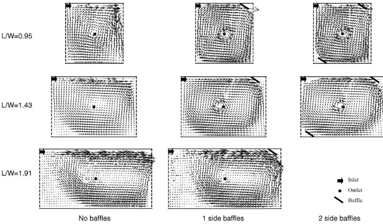
(10) 1. General introduction. General drain Jet. Influent. Drain. Figure 1.2: The mixed-cell raceway (Watten et al., 2000).. Another strategy for improving biosolids removal in rectangular tanks is to use vertical baffles to increase velocity and facilitate the removal of settled biosolids (Westers and Pratt, 1977; Boerson and Westers, 1986; Kindschi et al., 1991; Barnes et al., 1996; True et al., 2004). However, baffles can also contribute to fin erosion (Barnes et al., 1996) and affect the distribution of fish size in the tank (Kindschi et al., 1991). New rectangular tank designs have been used since the 1990s to increase the efficiency of water consumption and to optimise the use of space. Examples include the shallow raceway systems (SRSs) developed by Strand and ∅iestad (1997). SRSs typically use a very shallow water depth (tested with water levels of 7 mm for fish of approximately 100 mg, and 25 cm for fish above 2 kg), high velocities and high densities (∅iestad, 1999). The main disadvantage of this design is the low oxygen level in the tank due to the small volume of water volume used, which leads to a very short response time if the oxygenation system fails. Oxygen supersaturation must therefore be maintained at the water inlet, which increases the losses due to diffusion between the air and water. Several devices have been developed for concentrating solid wastes in rectangular systems. Wong and Piedrahita (2003) described a device that is placed close to the water outlet in raceways and creates the same effect as a dual-drain system (typical of circular tanks). The device produces rotational velocities downstream of the raceways, sweeps stable solids towards collection areas, and is capable of removing 40-50% of the settleable material with 5-10% of the total water circulating. 1.2.3. Velocity in rearing tanks If the velocities inside a tank can be controlled, it is easier to adjust the tank configuration to produce the desired fish swimming speed for maintaining general health, muscle tone and respiration, which varies according to the size and species of fish (Woodward and Smith, 1985; Watten and Johnson, 1990; Timmons and Youngs, 1991; Losordo and Westers, 1994). The velocity in the tank also needs to be controlled to make sure that the tank bottom is free of biosolids, since these waste particles consume oxygen and could create hypoxic conditions. A good water inlet and outlet design allows users to control the velocities and, by extension, the general flow conditions inside the tank (Tvinnereim and Skybakmoen, 1989). The water velocity needed to maintain self-cleaning 8.

(11) 1. General introduction. properties ranges from 3 to 40 cm s-1 varying greatly according to the physical properties of the biosolids (Burrows and Chenoweth, 1970; Boersen and Westers, 1986; Tvinnereim, 1988; Timmons and Young, 1991). The presence of fish in the tank can reduce the velocities needed to maintain self-cleaning properties, since more efficient cleaning has been demonstrated in circular tanks stocked with fish (Timmons et al., 1998; Lekang et al., 2000). For salmonids, the optimal velocities for fish health were found to be between 0.5 and 2 times the fish body length per second (BL s-1) (Timmons and Youngs, 1991; Losordo and Westers, 1994). The higher swimming speeds that can be attained in circular tanks were found to improve the growth rate and food conversion efficiency of teleost fish (Davison, 1997). Timmons and Youngs (1991) provided the following equation for predicting safe, nonfatiguing water velocities for salmonids:. v safe ≤. 5.25 BL0.37. Equation 1.1. where BL is the fish body length in cm and vsafe is the maximum design velocity (approximately 50% of the critical swimming speed) in fish body lengths s-1.. The average velocity in rectangular tanks can be calculated easily using Equation 1.2:. ν=. RL 3600. Equation 1.2. where v is the velocity (m s-1), R is the rate of exchange (h-1) and L is the length of the raceway (m).. However, the local velocity magnitudes can vary considerably from the average velocities in the longitudinal axis, due to the presence of unexpected eddies and dead volumes. The average velocity around the centre of a tank with a circular flow pattern is controlled by the impulse force and affected by the water inlet discharge and velocity (Tvinnereim and Skybakmoen, 1989) (Equation 1.3): Fi = ρ Q (v 2 −v1 ). Equation 1.3. where Fi is the impulse force, ρ is the density, Q is the discharge, v2 is the water velocity inlet and v1 is the mean circulation velocity.. Variations in discharge (flow rate) and section of water inlet orifices affect the impulse force and therefore control the horizontal circulation velocity. Timmons et al. (1998) reported that the mean circulation velocity (v1) is proportional to the inlet velocity (v2) for a specific circular tank. 1.2.4. Study of tank hydrodynamics There are various techniques for studying tank hydrodynamics. The most common techniques in the aquaculture field are residence time distribution (RTD) analysis (Burley and Klapsis, 1985; Watten and Beck, 1987; Watten and Johnson, 1990; Cripps and Poxton, 1993; Watten et al., 2000; Rasmussen and. 9.

(12) 1. General introduction. McLean, 2004; Rasmussen et al., 2005; Lunger et al., 2006) and tracer tests in which the tracer concentration is measured at different points in the tank (Burrows and Chenoweth, 1955; Tvinnereim, 1988; Tvinnereim and Skybakmoen, 1989). RTD provides accurate information about the flow behaviour inside tanks. The residence time of an element of fluid is the amount of time it spends in the vessel or tank, which is evaluated by examining the temporal evolution of a tracer that has been added to the tank (Levenspiel, 1966). Different fluid elements spend different amounts of time in the tank, so a distribution of residence times is produced. RTD curves are obtained by injecting a known amount of tracer at the water inlet and measuring the tracer concentration at the outlet. The technique is used to assess tank mixing and detect bypass currents and dead volumes and can be carried out while fish are present. However, RTD analysis cannot provide a detailed model of the velocity field. Tank hydrodynamics can also be studied by taking water velocity measurements at several points. The measurements can be taken using propeller velocity probes (Burley and Klapsis, 1985), electromagnetic current meters (Watten et al., 2000) or new techniques such as acoustic Doppler velocimetry (ADV), which was introduced in the 1990s. ADV has been used to measure water velocity in aquaculture tanks (Odeh et al., 2003; Davidson and Summerfelt, 2004; Labatut et al., 2007a; 2007b) and in quiescent zones (Viadero et al., 2005). Acoustic Doppler velocimeters provide accurate flow measurements, but the measurement points should not be too high in the tank. In addition, the probe can disrupt the flow. Water velocity measurements at a specific point can be taken while fish are present, although there are some restrictions and it must be taken into account that fish activity could affect the results. Computational fluid dynamics (CFD) can be used to describe the flow field in a tank in two or three dimensions, but the results need to be verified in subsequent laboratory or field studies. This technique has been used in river engineering (Nicholas and Smith, 1999), in sedimentation tank design (Stovin and Saul, 1996, 1998; Faram and Harwood, 2002; Adamsson et al., 2003), in the study of flow patterns in open channels (Wu et al., 2000), and in the field of aquaculture to study water flow and sediment transport in raceways (Peterson et al., 2000; Huggins et al., 2004; 2005). Other techniques introduced in the 1990s include particle velocimetry techniques such as particle tracking velocimetry (PTV). PTV is a non-intrusive method in which tracer particles are used to describe the flow pattern. Its main advantage is that a full flow field is obtained in a two-dimensional cross section of flow after image processing. However, it cannot be used in large tanks or when fish are present, since the tracer particles could harm them. PTV techniques have been used successfully in different fields of engineering (Sveen et al., 1998; Grue et al., 1999; Uijttewaal, 1999; Montero et al., 2001, Chang et al., 2002). The method has not yet been used to evaluate flow patterns in aquaculture tanks. Although some of these techniques can be used in real (field-scale) facilities (Table 1.1), most analyses are made at the laboratory scale because 10.

(13) 1. General introduction. modifications can be made more easily and more quickly. The results obtained with models are then transferred to larger tanks so that the scale effects can be evaluated. Table 1.1: Techniques used to study tank hydrodynamics and range of applications. Technique Residence time distribution Velocity measurement at a given point Particle velocimetry techniques Computational fluid dynamics. Full flow field. Laboratory scale. Field scale. With fish. NO. YES. YES. YES. NO. YES. YES. With restrictions. YES. YES. NO. NO. YES. --. --. --. The flow conditions in a physical model are comparable to those in the prototype if the model has a similar shape (geometry), motion (kinematics) and forces (dynamics). Similarity analysis is essential for transferring results to other, geometrically similar tanks at a different scale. Geometric similarity is determined by the length (L), area (A) and volume (V) of the tank. The characteristic length ratio (λL, Equation 1.4) between fullscale (LF) and model (laboratory-scale) tanks (LM) must be constant for similarity to exist.. λL =. LF LM. Equation 1.4. Kinematic similarity implies that the ratios between characteristic full-scale (vF) and model velocities (vM) must be constant (λv) (Equation 1.5). Dynamic similarity also implies a constant ratio (λF) between full-scale (FF) and model forces (FM) (Equation 1.6).. λv =. vF vM. Equation 1.5. λF =. FF FM. Equation 1.6. Froude and Reynolds numbers are the main criteria used when the results from hydrodynamic studies with a tank model are transferred to a full-scale prototype. The Reynolds number relates the inertial forces to the viscous forces (Equation 1.7): Re =. vL. υ. Equation 1.7. where v is the water velocity, L is the characteristic length (usually water depth) and υ is the kinematic fluid viscosity.. 11.

(14) 1. General introduction. By scaling up model velocities using the Reynolds criteria, we obtain. vM LM. v F LF υm = υF ,. and by taking υ M =υ F , we obtain v F = v M LM. LF. = v M λ−L1 .. The Froude number relates the inertial forces to the gravitational forces (Equation 1.8) and is the most common dimensionless number used in openchannel hydraulics (free-surface flow); gravitational effects are dominant, so the effect of viscosity can be disregarded:. Fr =. v. Equation 1.8. (g L ) 2 1. where v is the water velocity, L is the characteristic length (usually water depth) and g is the acceleration due to gravity. By scaling up the model velocities using the Froude criteria, we obtain. vM. vF. 1/ 2. L ⎞ we obtain v F = v M ⎛⎜ F ⎟ L M ⎠ ⎝. 1/ 2. LM. 1/ 2. =. LF. gM. 1/ 2. gF. 1/ 2. ,. and by taking g M = g F ,. = v M λ1L/ 2 .. The velocity obtained for a particular fluid (identical viscosity) will differ considerably depending on whether the Froude or Reynolds criteria are used (according to the Reynolds criteria, v F = v M λ−L1 ; according to the Froude criteria, v F = v M λ1L/ 2 ). Care should be taken when transferring results. Laboratory models with high Reynolds numbers are often used to minimise the influence of viscous forces on the flow. Consequently, it is common to use the Froude criteria and to verify the error induced by the effect of viscous forces in full-scale prototypes. 1.2.5. Effect of fish swimming activity on tank hydrodynamics Fish swim either by body/caudal fin (BCF) movements or median/paired fin (MPF) propulsion (Videler, 1993). When fish swim, the surrounding water moves at the same velocity. Water beyond the boundary layer is not dragged along in the swimming direction, and a velocity gradient is generated, which causes free shear. When the flow changes from laminar to turbulent, water sheets that move at different velocities fail to follow the contour of the body and the flow separates into circulating masses of water called eddies or vortices (Figure 1.3), which increase turbulence and mixing.. 12.

(15) 1. General introduction. u. Figure 1.3: Eddies generated behind a swimming fish. A jet flow with alternating direction between the vortices can be seen (Sfakiotakis et al., 1991).. The turbulence generated by fish movement affects the tank hydrodynamics. Studies have been carried out to analyse the effect of fish activity and distribution on water homogeneity (Davidson and Summerfelt, 2004; Rasmussen et al., 2005; Lunger et al., 2006) and sediment dynamics (Brinker and Rösch, 2005). Fish activity can have a significant effect on tank mixing, particularly in intensive farming systems where high fish densities are common. Higher fish densities generate higher turbulence (Lunger et al., 2006), which can often be sufficient to keep biosolids in suspension or to facilitate resuspension from the tank bottom, even with low current velocity or a mean velocity of zero. Fish activity has been studied using several different methods, such as acoustic telemetry (Bégout and Lagardère, 1997; 2004; Schurmann et al., 1998; Bauer and Schlott, 2004), acoustic monitoring (Conti et al., 2006), image processing (Fitzsimmons and Warburton, 1992; Kato et al., 1996), visual observation (Wagner et al., 1995) and infrared sensors (Iigo and Tabata, 1996; Sánchez-Vázquez et al., 1996). However, none of these methods provide a measurable parameter of the turbulence generated by fish swimming activity and all of them have certain restrictions (Table 1.2): most can only be used with a small number of fish, and some are intrusive or subjective methods. Furthermore, fish behaviour, especially in schooling species, may be different when fish are reared at different densities (e.g. rainbow trout (Oncorhynchus mykiss L.), Bégout and Lagardère, 2004)), or when a fish is isolated rather than in a group (e.g. mullet (Mugil cephalus L.), Fitzsimmons and Warburton, 1992; sea bass (Dicentrarchus labrax L.), Bégout and Lagardère, 1997; Bégout et al., 1997). It would very useful to develop a method for studying fish swimming movements and behaviour in more natural conditions. This could be done using new and innovative techniques and technologies (Peake and MacKinlay, 2004). The method should provide a measurable turbulence parameter and should be suitable for use with high densities to quantify the effect of fish swimming activity on hydrodynamics and on the sedimentation and resuspension of biosolids in aquaculture tanks.. 13.

(16) 1. General introduction. Table 1.2: Techniques used to study fish activity and their pros and cons. Cons. Turbulence measurement?. -Only with a low number of fish -Problems with tagging small fish or flatfish. NO. Pros Acoustic telemetry Acoustic monitoring Image processing Visual observation Infrared sensors. -Describes fish path -Velocity is known. -Determines fish density and behaviour -Only with a low number of fish -No fish handling -Only with a low number of fish -Describes fish path -Problems with flatfish -Velocity is known overlapping -No technology needed -Subjective -No fish handling -Only with a low number of fish -Poor information obtained -No fish handling -Only with a low number of fish. 14. NO NO NO NO.

(17) 1. General introduction. 1.3. SEDIMENTATION AND RESUSPENSION OF AQUACULTURE BIOSOLID WASTES Aquaculture sediments in rearing tanks are mainly organic. They are commonly defined as biosolids, which include faeces and non-ingested feed. When biosolids accumulate on the tank bottom, they can promote the spreading of pathogens and the degradation of water quality due to oxygen consumption. In addition, when the biosolids dissolve or leach into the water, they increase the concentration of nitrogenous compounds, which can affect fish growth and welfare. Some biosolids are removed immediately from rearing areas by the water current, but others settle on the tank bottom and need to be resuspended before they can be removed. The following sections discuss the forces that affect the resuspension of solid particles in a tank. They also describe the characteristics of biosolids and the different techniques for studying resuspension and sedimentation processes in cohesive sediment dynamics. 1.3.1. Characterisation of settleable aquaculture wastes Sediment classifications can be based on various characteristics, such as particle size, colour, texture and organic content. Sediments are classified as cohesive (mainly organic) material or noncohesive (mainly mineral) material depending on their organic content. Mineral sediment transport has been widely studied (Raudkivi, 1990; Van Rijn, 1993; 2005; Chanson, 1999), but cohesive sediments are more difficult to characterise because their properties can change over the time (due to aggregation and disaggregation). Physical characterisations of sediments are usually based on particle size, specific gravity and sedimentation rate. Sediment size and specific gravity can be determined easily for mineral particles using different techniques (sieves, laser, image analysis, etc.). However, organic materials such as aquaculture biosolids are more difficult to characterise because of three main properties that differentiate them from marine and river sediments: high proportion of organic components, low specific gravity and high cohesiveness. High cohesiveness promotes aggregation, but the particle aggregates are very easy to disrupt and can change their physical characteristics over time, which makes it more difficult to study the dynamics of biosolids. In addition, biosolids can consolidate if they are left undisturbed on the tank bottom (Mehta et al., 1989; Zreik et al., 1998; Orlins and Gulliver, 2003). When collecting biosolids prior to characterisation, it is important to ensure that their physical properties are not disturbed. Several collection methods can be used: manual stripping (massage of the ventral abdominal wall after fish have been anesthetised) (Chen et al., 1999; Wong and Piedrahita, 2000), dissection of the intestine (Chen et al., 1999), hand-net collection (Chen et al., 2003), traps under cages (Magill et al., 2006) and direct collection from quiescent zones (Merino et al., 2007a). The properties of aquaculture biosolids have been widely studied, mainly by determining the sedimentation rate (Chen et al., 1999; Wong and Piedrahita, 15.

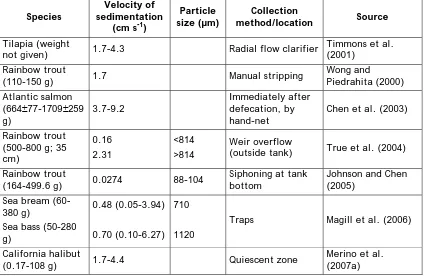
(18) 1. General introduction. 2000; Chen et al., 2003) and particle size (Chen et al., 1993; Brinker et al., 2005). However, aquaculture biosolids vary considerably according to fish species (Magill et al., 2006), fish diet (Merino et al., 2007b), and the feeding strategies adopted (Cho and Bureau, 2001). It is very difficult to define universal characteristics. Tables 1.3 and 1.4 summarise the physical characteristics of aquaculture biosolids obtained from fish of different species and sizes. Table 1.3: Specific gravity of biosolids in aquaculture facilities. Species. Collection method/location. Specific gravity. Source. Brook trout (approx. 50 g) 1.190. Bottom of screen (outside tank). Chen et al. (1993). Atlantic salmon smolts (weight and length not given). Near the drain. Patterson et al. (2003). Weir overflow (outside tank). True et al. (2004). 1.050-1.153. Rainbow trout (500-800 g; 1.250 35 cm). Table 1.4: Sedimentation rate and particle size of biosolids in aquaculture facilities. Species. Velocity of sedimentation (cm s-1). Particle size (µm). Collection method/location. Source. Tilapia (weight not given). 1.7-4.3. Radial flow clarifier. Timmons et al. (2001). Rainbow trout (110-150 g). 1.7. Manual stripping. Wong and Piedrahita (2000). Immediately after defecation, by hand-net. Chen et al. (2003). Atlantic salmon (664±77-1709±259 3.7-9.2 g) Rainbow trout (500-800 g; 35 cm). 0.16 2.31. <814 >814. Weir overflow (outside tank). True et al. (2004). Rainbow trout (164-499.6 g). 0.0274. 88-104. Siphoning at tank bottom. Johnson and Chen (2005). Traps. Magill et al. (2006). Quiescent zone. Merino et al. (2007a). Sea bream (60380 g) Sea bass (50-280 g) California halibut (0.17-108 g). 0.48 (0.05-3.94) 710 0.70 (0.10-6.27) 1120 1.7-4.4. Recent studies have focused on the inclusion of binders in feed formulations (Brinker et al., 2005; Brinker, 2007) to prevent faeces disintegration, which can promote leaching (Stewart et al., 2006).. 16.

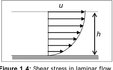
(19) 1. General introduction. 1.3.2. Basics of sediment transport Sediment resuspension in natural systems is driven by bed shear stress τ (the force exerted per unit area parallel to a bed). The shear stress τ of the flow is the force that lifts particles from the bed and entrains them in the flow. If the bed shear stress exceeds a threshold value for a particular particle size and composition (critical shear stress τc), the particle will be lifted from the bed and carried by the flow. When the bed shear stress drops below the threshold value, the entrained particle will drop back to the bed. Consequently, the bed shear stress determines whether resuspension or sedimentation occurs. Shear stress is observed in both laminar and turbulent flows. The molecule path is parallel in laminar flow, and lower velocities are observed close to the solid boundary due to friction (Figure 1.4). The velocity gradient produces the shear stress (Equation 1.9). Shear stress in laminar flows is caused by water viscosity, so it is commonly referred to as viscous shear stress (τµ).. τµ =. du µ dh. Equation 1.9. where du is the flow velocity gradient (m s-1), dh is the water depth (m) and µ is the fluid dynamic viscosity (kg m-1 s-1).. The magnitude of the shear stress in laminar flows is determined by the velocity gradient (du/dh) (Figure 1.4). u. h. Figure 1.4: Shear stress in laminar flow.. In turbulent flow, molecules move horizontally and vertically and generate continuous mixing (a stochastic process in which the velocities fluctuate in space and time). The instantaneous velocity components in the x-axis in turbulent flows can be defined as:. U = u +u '. Equation 1.10. where U is the instantaneous velocity, u is the time-average velocity and u’ represents the instantaneous velocity fluctuations.. Transfer of movement up and down is done by macroscale processes. Movements of molecules cause a continuous exchange of momentum from one portion of fluid to another. This momentum exchange generates the turbulent shear stress (τt) or Reynold stress (Equation 1.11):. 17.

(20) 1. General introduction. τ t = − ρ u 'w'. Equation 1.11. where ρ is the fluid density (kg m-3), u’ represents the instantaneous velocity fluctuations in the x-axis (m s-1) and w’ represents the instantaneous velocity fluctuations in the z-axis (m s-1).. Equation 1.11 can be used to calculate the turbulent shear stress, but the total shear stress (τT) in turbulent flows is defined as the sum of the viscous and turbulent shear stresses and is expressed as:. τ T =τ µ +τ t =. du du µ+ η dh dh. Equation 1.12. where η is the apparent or eddy viscosity (kg m-1 s-1).. In aquaculture tanks, the bed shear stress generated by circulating water can combine with the free shear stress from the inflow water and the free shear stress from fish swimming activity to promote resuspension. It is interesting to examine how turbulence affects the terminal fall velocity of suspended biosolid particles. There is a great deal of disagreement on this issue, since it is not clear what type of vertical velocity distribution could be defined in natural conditions or whether turbulence increases or reduces the particle fall velocity (Van Rijn, 1993). 1.3.3. Study of biosolid dynamics To determine rates of sedimentation or resuspension, a shear stress has to be generated and the amount of resuspended or settled material is measured. Various techniques have been used to measure sediment accumulation in natural environments (Bloesch, 1994; Thomas and Ridd, 2004). These include using optical or acoustic instruments, taking instantaneous multiple-point water samples, and using sediment traps and/or sediments cores. Sediment traps are the most frequently used technique (Flower, 1991; Kozerski, 1994) because they provide an easy way of collecting particles, although they can overestimate the volume of resuspended sediment if the design is poor (i.e. if the traps do not have an appropriate depth/diameter ratio). Methods based on annular flumes or tanks (Nowell et al., 1981; Portela and Reis, 2004; Droppo et al., 2007; Neumeier et al., 2007; Traynum and Styles, 2007) were used to study sediment resuspension in the laboratory experiments after collection. These methods produced horizontally and vertically sheared Couette flows. In Couette flows, the shear stress is constant and generated by the laminar flow of a viscous liquid in the space between two parallel plates, one of which is moving relative to the other. Oscillating grids can also be used to determine resuspension. These types of grids produce no net flow, but the turbulence generated by the oscillations generates a shear stress that decreases with distance from the grid. The turbulence produced in these types of devices is expressed as the root mean square (RMS) of the velocity. RMS is a statistical measure of the velocity fluctuation (Equation 1.13): 18.

(21) 1. General introduction. ∑ (v −v ) n. RMS =. i =1. i. n. ave. 2. Equation 1.13. where vi is the instantaneous velocity measurement, vave is the mean velocity of the flow and n is the number of instantaneous velocity measurements. RMS is expressed in velocity units.. Aquaculture tanks can contain dead zones in which the mean flow is zero. However, even in these cases, a free shear flow induced by fish activity could be sufficient to resuspend biosolids. Oscillating grids can provide extremely useful information about the turbulence needed to resuspend aquaculture biosolids, which are highly cohesive. To define the self-cleaning conditions of a tank and develop strategies for keeping tanks clean, it is useful to know the turbulence needed to maintain biosolids suspended in the water column, the turbulence needed to resuspend those biosolids that have settled, and the turbulence generated by fish swimming activity.. 19.

(22) 1. General introduction. 1.4. OBJECTIVES 1.4.1. General objective The main goal of this dissertation was to determine design criteria for aquaculture tanks that would produce optimal rearing conditions, ensure that biosolids are removed rapidly, and optimise the use of space and water. The dissertation covers tank hydrodynamics, fish activity and biosolid sedimentation dynamics and highlights the relationship between them (Figure 1.5). We assessed the effect of flow pattern and fish swimming activity on the hydrodynamic conditions of aquaculture tanks and studied environmental homogeneity and sedimentation processes. Geometry Inlet Outlet. TANK DESIGN. Others (Colour, illumination, materials...). Hydrodynamics. Biosolid dynamics. Fish growth and welfare. Fish distribution and activity. Figure 1.5: Variables involved in tank design and relationships between hydrodynamics, fish activity and biosolid dynamics.. The tank geometry and water inlet and outlet characteristics determine the hydrodynamics in the absence of fish. The tank hydrodynamics affect the rearing environment and fish behaviour. Fish distribution and activity in the tank also affect the hydrodynamic conditions; mixing and resuspension of biosolids increase when pelagic fish are present. 1.4.2. Specific objectives of the articles in this dissertation. •. The influence of the geometry and water inlet devices on the flow pattern of the most common aquaculture tanks will be analysed to define design criteria that will improve the rearing conditions and optimise the use of water (Article 1). Oca, J., Masaló I., Reig, L. (2004) Comparative analysis of flow patterns in aquaculture rectangular tanks with different water inlet characteristics. Aquaculture Engineering 31 (3-4), pp. 221-236. •. Design criteria will be established for ‘rotating-cell rectangular aquaculture tanks’, which combine the advantages of rectangular and circular tanks (Article 2). Oca, J., Masaló, I. (2007) Design criteria for rotating flow cells in rectangular aquaculture tanks. Aquacultural Engineering 36 (1), pp. 36-44. 20.

(23) 1. General introduction. •. A method for studying fish activity by measuring the turbulence generated by swimming will be developed. This will provide a means of analysing the relationship between the turbulence produced by fish swimming activity and the rearing conditions in the tank (Article 3). Masaló, I., Reig, L., Oca, J. (2008) Study of fish swimming activity using Acoustical Doppler Velocimetry (ADV) techniques. Aquacultural Engineering 38 (1), pp 43-51. •. The turbulence needed to resuspend aquaculture biosolids and to keep them suspended in the water column will be analysed using a vertically oscillating grid adapted to the specific characteristics of aquaculture biosolids (Article 4). Masaló, I., Guadayol, O., Peters, F., Oca, J. (2008) Analysis of sedimentation and resuspension processes of aquaculture biosolids using an oscillating grid. Aquacultural Engineering 38 (2), pp 135-144. 21.

(24) 2. PUBLISHED ARTICLES INCLUDED IN THIS DISSERTATION.

(25) 2.1. Oca, J., Masaló I., Reig, L. (2004) Comparative analysis of flow patterns in aquaculture rectangular tanks with different water inlet characteristics. Aquaculture Engineering 31 (3-4), pp. 221-236..

(26) Aquacultural Engineering 31 (2004) 221–236. Comparative analysis of flow patterns in aquaculture rectangular tanks with different water inlet characteristics Joan Oca∗ , Ingrid Masaló, Lourdes Reig Departament d’Enginyeria Agroalimentària i Biotecnologı́a, Centre de Referència en Aqüicultura, de la Generalitat de Catalunya, Universitat Politècnica de Catalunya (U.P.C.), Urgell 187, 08036 Barcelona, Spain Received 25 July 2003; accepted 14 April 2004. Abstract The objective of the work is to improve the design rules of rectangular aquaculture tanks in order to achieve better culture conditions and improve water use efficiency. Particle tracking velocimetry techniques (PTV) are used to evaluate the flow pattern in the tanks. PTV is a non-intrusive experimental method for investigating fluid flows using tracer particles and measuring a full velocity field in a slice of flow. It is useful for analysing the effect of tank geometries and water inlet and outlet emplacements. Different water entry configurations were compared, including single and multiple waterfalls and centred and tangential submerged entries. The appearance of dead volumes is especially important in configurations with a single entry. Configuration with a single waterfall entry shows a zone of intense mixing around the inlet occupying a semicircular area with a radius around 2.5 times the water depth. A centred submerged entry generates a poor mixing of entering and remaining water, promoting the existence of short-circuiting streams. When multiple waterfalls are used, the distance between them is shown to have a strong influence on the uniformity of the velocity field, increasing noticeably when the distance between inlets is reduced from 3.8 to 2.5 times the water depth. The average velocities in configurations with multiple waterfalls are very low outside the entrance area, facilitating the sedimentation of biosolids (faeces and non-ingested feed) on the tank bottom. The horizontal tangential inlet allows the achievement of higher and more uniform velocities in the tank, making it easy to prevent the sedimentation of biosolids. © 2004 Elsevier B.V. All rights reserved. Keywords: Particle tracking velocimetry; Aquaculture tank design; Flow pattern. ∗. Corresponding author. Tel.: +34-934137532; fax: +34-934137501. E-mail address: joan.oca@upc.es (J. Oca).. 0144-8609/$ – see front matter © 2004 Elsevier B.V. All rights reserved. doi:10.1016/j.aquaeng.2004.04.002.

(27) 222. J. Oca et al. / Aquacultural Engineering 31 (2004) 221–236. 1. Introduction The design of tanks in inland aquaculture systems is an essential issue in order to achieve optimal conditions for fish and minimise waste discharge into the environment, and has been dealt with by different authors (among others Wheaton, 1977; Cripps and Poxton, 1992, 1993; Lawson, 1995; Ross et al., 1995; Timmons et al., 1998; Watten et al., 2000). A comprehensive approach to the tank design should include the geometry and the water inlet and outlet characteristics, which together will determine the flow pattern. Two types of geometry are used in the construction of aquaculture tanks: circular and rectangular. Circular tanks are frequently self-cleaning. The circular flow pattern moves biosolids (non-ingested feed and faeces) to the central outlet, where they are swept out in the outlet current. A downstream settling zone is required to collect biosolids from these ponds. Environmental conditions are usually very uniform in this kind of tank due to the effective mixing of water achieved (Timmons et al., 1998). In rectangular tanks, flow pattern is much more unpredictable, heavily depending on the tank geometry and the characteristics of water inlets. In this kind of tank the majority of biosolid particles usually settle on the bottom, especially at low fish densities, when the turbulence produced by fish movement is not very great. In rectangular tanks it is also much more usual to find heterogeneous culture environments caused by the lack of mixing uniformity, which generates dead and by-passing volumes. These conditions will provoke disparity in fish distribution and fish quality and in some cases an increase in aggressive behaviour of fish (Ross et al., 1995). Despite the number of problems above described, rectangular tanks are widely used in aquaculture farms on account of the fact that they are easier to construct, facilitate fish handling and adapt to usual plot geometries. The water inlet is usually made through submerged horizontal inlets or through waterfalls placed in one extreme of the tank. The influence of inlet and outlet arrangements in the hydraulic behaviour of the tanks has been widely studied in circular tanks (Klapsis and Burley, 1984; Tvinnereim and Skybakmoen, 1989; Timmons et al., 1998) but scarcely in rectangular tanks. Some authors have suggested inlet configurations placed along the sidewalls of the rectangular tanks to increase the mixing flow conditions and provide self-cleaning proprieties (Watten and Beck, 1987; Watten et al., 2000). In general, two ideal flows can be defined for rectangular tanks: the “plug flow” and the “mixing flow”. In the “plug flow” there is no mixing or diffusion along the flow path and the maximal waste concentration is found in the outlet. In the “mixing flow” the exit stream from the tank has the same composition as the fluid within the tank (Levenspiel, 1979), providing greater uniformity conditions due to the intense mixing. Nevertheless, in rectangular aquaculture tanks it is very usual to have deviations from these two ideal flow patterns, existing short-circuiting streams leaving the tank without mixing well with remaining water, and dead volumes with low renovation rates. Both phenomena will contribute to a low efficiency in water use and to make the treatment of wastes more difficult. Many authors have evaluated the hydraulic behaviour of some aquaculture tanks using methods like the analysis of residence time distribution (RTD) (Burley and Klapsis, 1985; Watten and Beck, 1987; Watten and Johnson, 1990; Cripps and Poxton, 1993; Watten.

(28) J. Oca et al. / Aquacultural Engineering 31 (2004) 221–236. 223. et al., 2000) or tracer tests (Burrows and Chenoweth, 1955; Tvinnereim and Skybakmoen, 1989). These evaluations are based on the temporal evolution of a measurement that is a consequence of the flow pattern (concentration of a tracer), but none of them provide a quantitative description of the flow pattern. As a consequence, these methods are useful for the evaluation of existing tanks, measuring the mixing intensity and detecting flow anomalies like short-circuiting or dead volumes, but not to give useful information for improvement of the tank design. The direct measurement of velocities at various points of the tank volume has also been used by some authors (Burley and Klapsis, 1985; Watten et al., 2000) but the number of measurements is necessarily small and the flow is inevitably disturbed by the presence of the measuring probe. In the last decade, the experimental methods for characterising flow patterns have improved greatly due to availability and the increase in computer power, which has allowed the development of particle velocimetry techniques. These methods use tracer particles and measure a full velocity field in a two-dimensional slice of a flow. One of these techniques, called “particle tracking velocimetry” (PTV), utilises time series of images, estimates the position of the particles and measures their displacement. It has been used in many works in order to characterise flow patterns in the field of building ventilation (Montero et al., 2001), river engineering (Uijttewaal, 1999) and marine engineering (Sveen et al., 1998; Grue et al., 1999; Chang et al., 2002). Results are usually presented as a vectors map where the length of every arrow is proportional to the velocity. The application of PTV to other fields, such as the design of aquaculture tanks, could provide useful information in order to improve the design rules, thus aiding the achievement of better culture conditions and water use efficiency. Taking advantage of PTV techniques, the goal of this work has been the evaluation of the flow pattern obtained in rectangular tanks, to analyse the effect of geometrical characteristics and inlet and outlet emplacement.. 2. Material and methods 2.1. Flow visualisation The experiments were carried out using a rectangular tank made of transparent methacrylate, 100 cm long and 40 cm wide. The water depth was always close to 5 cm. Exchangeable gates placed in the tank extremes allowed the water inlet and outlet characteristics to be changed easily. The circulation of water was achieved using a volumetric pump equipped with a variable speed motor, in order to adjust the recirculation flow rates (Fig. 1). The water volume was “seeded” with small particles of pliolite (Eliokem, pliolite S5E), a granular material with good reflective properties and density approximately 1.05 g cm−3 . The particles used passed through a US Standard Sieve #18 screen (1.00 mm) but were retained on a #35 screen (0.50 mm). The used amount of dry pliolite was around 1 g l−1 . In order to give neutral buoyancy to these particles, they must be submerged in a wetting agent to reduce the surface tension and sodium chloride must be added to the water tank (around 65 g l−1 ) to equal water and pliolite densities..

(29) 224. J. Oca et al. / Aquacultural Engineering 31 (2004) 221–236. Fig. 1. Recirculating water system and dimensions of the tank.. The following step is to illuminate a slice of flow (around 5 mm thick) in the section where the velocity field has to be obtained. Some vertical and horizontal sections were analysed in each experiment for a better understanding of the three-dimensional pattern. Following the pliolite particles from this slice during a short time period, the bi-dimensional velocity field in the lighted slice can be found. In order to achieve a sufficiently good resolution of the images, the tank analysis was divided into two halves, analysing separately the half closer to the inlet and the half closer to the outlet. The analysis of both halves was made at different times, that is why, when the flow pattern is time dependant, the flow pattern of the first half may not fit the flow pattern in the second half. 2.2. Particle tracking and analysis In order to track particles, the images of the flow must be captured, the particles must be located within these images, and the relationship between particles in successive images must be determined. The illuminated region of the flow was recorded on a Super VHS videotape using a monochrome CCD video-camera (COHU 4912). To track the particles, the videotape was replayed and the images were captured by digitising the video using a frame grabber card (Data Translation 2861). The control of the video recorder (Panasonic AG-7350) was carried out by the same computer in which the frame grabber card was installed, using a specific software for this application (Digimage). The software defines a particle as an area of an enhanced image satisfying a number of criteria, based on the intensity, size and shape of the particles. Once all the particles in an image have been found, they need to be related back to the previous image to determine which particle image is which physical particle. The displacement, velocity and trace of each particle are determined from sequences of frames. The summarisation of the data obtained is made by using an analysis package (Trk2DVel), which provides the results in the form of graphical output or statistics of the flow (Dalziel, 1999)..

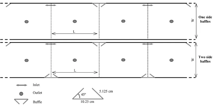
(30) J. Oca et al. / Aquacultural Engineering 31 (2004) 221–236. 225. Fig. 2. Tank configurations analysed.. 2.3. Tank configurations analysed The tank configurations analysed are presented in Fig. 2. 1. 2. 3. 4.. A single upright waterfall (centred in one of the shorter walls of the tank). A single horizontal submerged entry (centred in one of the shorter walls of the tank). Multiple upright waterfalls (uniformly distributed in one of the shorter walls of the tank). Tangential inlets placed in the centre of the longer side wall, in order to perform two large eddies.. The outlets were always placed superficially in the centre of the opposite wall of the entry, except for configuration 4, where the outlets are placed in the centre of the eddies, at the tank bottom. Three different flow rates were used in configuration 1 in order to study the influence of the flow rate in the flow pattern observed around the waterfall. In configuration 3, two and three inlets uniformly distributed were studied, corresponding to a distance between inlets of 3.8 and 2.5 times the depth, respectively. The different flow rates used with every configuration can be seen in Table 1, together with the water depth and the exact emplacement and characteristics of the inlet. To transfer the results to other geometrically similar tanks, the main criteria to be used will be the Froude number (Fr = v/(gL)1/2 ), which relates inertial forces to gravity forces and the Reynolds number (Re = Lv/ν), which relates inertial forces to viscous forces. If the same fluid (i.e. water) is used in both the model and the full-scale prototype it is not possible to keep both the Froude and Reynolds numbers in the model and full-scale. In free-surface flows gravity effects are dominant, and model-prototype similarity is usually performed with the Froude number, neglecting the effect of viscous forces. To have the same Froude number in two geometrically similar tanks with a length scale λL , the velocity scale (λv ) must be λv = λL0.5 , the flow rate scale (λf ) λf = λL2.5 , and the exchange rate scale λe must be λe = λL−0.5 . Thus, an exchange rate 9 h−1 in the analysed.

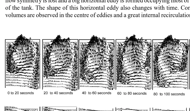
(31) 226. J. Oca et al. / Aquacultural Engineering 31 (2004) 221–236. Table 1 Flow rate, exchange rate and water depth in analysed configurations Distance between inlets/water depth. Flow rate (1 h−1 ). Water depth (cm). Velocity inlet (cm s−1 ). Exchange rate (h−1 ). Fall height (cm). Horizontal entry. –. 100. 5.0. 13.8. 5.0. –. Single waterfall. – – –. 95 140 182. 5.3 5.4 5.5. – – –. 4.5 6.5 9.1. 3. Multiple waterfalls. 3.8 2.5. 182. 5.5. –. 9.1. 2.5. Tangential inlets. –. 215. 6.0. 77.5. 9.0. –. model would correspond to 2 h−1 in a tank 20 times larger (20 m long × 8 m wide). This transfer would provide a good approximation to the flow pattern in the larger tank, but it should be verified through full-scale experiments due to the greater importance of viscous forces in the smaller tanks.. 3. Results and discussion The development of this section starts with a detailed description of the hydraulic aspects for each of the configurations evaluated in the present work. Later, all the configurations will be compared and the possible implications on fish culture discussed. 3.1. Configuration 1: a single upright waterfall With this configuration a vertical eddy is always formed close to the inlet in the way shown in Figs. 3 and 4. Fig. 3 shows a vertical section taken in the centre of the longitudinal axis of the tank, near the inlet, and two horizontal sections taken close to the free surface (A) and close to the tank bottom (B). In the vertical section, the vertical vectors corresponding to the entry waterfall are not plotted because they are out of range of velocity that can be detected by the equipment, but the eddy formed by this vertical flow is clearly shown. In the horizontal sections the velocity vectors are advancing in the bottom section and going back in the top section, creating a semicircular area of intense mixing around the waterfall with a radius equal to the eddy length. The length of the vertical eddy is not appreciably altered by the flow rate, as can be seen in Fig. 4 where the vertical eddies obtained with the three different flow rates are shown. This length is always close to two and a half times the water depth. Outside the above defined area of intense mixing, large horizontal eddies are formed along the length of the tank as can be observed in Fig. 5. Each eddy tends to occupy the whole width of the tank, with considerable dead volumes appearing in the eddy cores. Owing to these large eddies, the velocity field is very heterogeneous and the internal recirculation in the tank is very important..

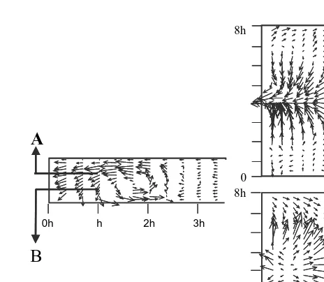
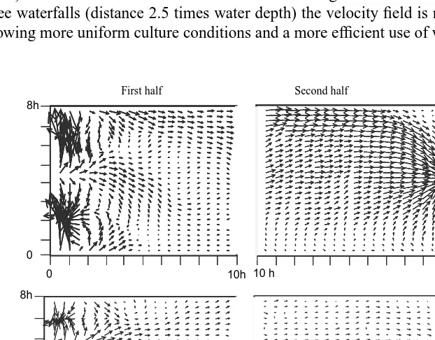
(32) J. Oca et al. / Aquacultural Engineering 31 (2004) 221–236. 227. 8h. (A). A 0 8h 0h. h. 2h. 3h. B (B). 0. Fig. 3. Velocity fields in a vertical section taken in front the single waterfall (left) and in the two horizontal sections A and B (right).. Fig. 6 shows a sequence of pictures with the flow patterns observed for 2 min, averaging 20 s in every picture. The great time dependence of the flow patterns observed with this kind of configuration must be highlighted. Eddies are continuously changing their shape and emplacement.. Fig. 4. Velocity fields in vertical sections of the first half of the tank with configuration 1, using different flow rates..

(33) 228. J. Oca et al. / Aquacultural Engineering 31 (2004) 221–236 First half. 8h. Second half. 0 0. 10h. 10 h. 20h. Fig. 5. Velocity fields in horizontal sections with configuration 1.. 3.2. Configuration 2: a single horizontal submerged entry The field of velocities in a horizontal section of the tank with this configuration is shown in Fig. 7. It can be seen that the plume formed by the entering water maintained its symmetry along the first quarter of the tank, which means along a length around five times the water depth. From this distance to 10 times the water depth the symmetry is progressively lost. At both sides of the plume, lateral eddies can be observed. In the second half of the tank, the flow symmetry is lost and a big horizontal eddy is formed occupying most of the second half of the tank. The shape of this horizontal eddy also changes with time. Considerable dead volumes are observed in the centre of eddies and a great internal recirculation of water must. Fig. 6. Sequence of flow pattern observed along 2 min with configuration 1..

(34) J. Oca et al. / Aquacultural Engineering 31 (2004) 221–236 First half. 8h. 229. Second half. 0 0. 10h. 10 h. 20h. Fig. 7. Velocity fields in horizontal sections with configuration 2.. be assumed. The flow pattern obtained is in accordance with the results obtained by Stovin and Saul (1994) using a propeller meter in a sedimentation tank with similar geometrical and inlet characteristics. The observed flow pattern also suggests the existence of an important short-circuit stream, resulting from the absence of an area of intense mixing between the entering water and the stored water. The short-circuit stream will not only increase the heterogeneity of environmental conditions inside the tank, but will also contribute to having low water use efficiency in open systems and will make water treatment in recirculating systems more difficult. Despite the described drawbacks with this kind of configuration, it is still very usual to find it in some inland grow-out marine fish farms. 3.3. Configuration 3: multiple upright waterfalls Two trials are evaluated in this configuration. The first with two waterfalls and the second with three waterfalls. The distance between waterfalls is, respectively, 3.8 and 2.5 times the water depth. Fig. 8 shows the flow pattern in two horizontal sections for each trial, one of them taken close to the free surface (top section) and the other close to the bottom (bottom section). Considering the results of configuration 1, where the eddy radius was always close to two and a half times the water depth, the analysed distances between inlets mean an overlapping of the expected single eddies around 50 and 100%, respectively. Observing the same figure, the effect of overlapping eddies in the flow pattern can be easily seen. In the top section, a horizontal plume is formed midway between two eddies. Meanwhile, in the bottom section, the flow in front of the waterfall seems to be mainly going back and the velocities perpendicular to the main flow direction seem to be higher when compared with the single waterfall configuration. A better understanding of this behaviour can be obtained by observing, in Fig. 9, two vertical sections placed midway between two entries (A) and in front of a water entry (B). In the first, most of the vectors are advancing and rising, forming the superficial plume. Meanwhile, in the second, most of the vectors are going back and down. This behaviour suggests that vertical eddies are formed in the direction perpendicular to the tank length, as shown in Fig. 10. These eddies will contribute to a better mixing of fluid in the first part of the tank and to a larger dissipation of the kinetic energy in this first part..

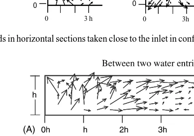
(35) 230. J. Oca et al. / Aquacultural Engineering 31 (2004) 221–236. Bottom section. Top section 8h. 8h. Two waterfalls. 0. 0 0. 0. 3h. 8h. 3h. 8h. Three waterfalls. 0. 0 0. 3h. 0. 3h. Fig. 8. Velocity fields in horizontal sections taken close to the inlet in configuration 3, with two and three waterfalls.. Fig. 9. Velocity fields in vertical sections in configuration 3. The first taken (A) between two water entries and (B) the second in front of water entry.. Fig. 11 shows that after the “mixing volume” produced in the entry, the observed flow is much more uniform in this kind of configuration than with the previous one, preventing the formation of large horizontal eddies and, therefore, the internal recirculation inside the tank..

(36) J. Oca et al. / Aquacultural Engineering 31 (2004) 221–236. a. 231. ~4 h. a. Plume. h. Intensive mixing volume. Fig. 10. Flow behaviour in a configuration with multiple waterfalls when the distance between eddies is around 2.5 times the water depth.. When comparing the flow pattern with two and three waterfalls, the main difference is the homogeneity in the velocity field. In the tank with two entries (distance 3.8 times water depth) the circulation at one of the tank sides is much higher than at the other side, while with three waterfalls (distance 2.5 times water depth) the velocity field is more homogeneous, allowing more uniform culture conditions and a more efficient use of water.. First half. Second half. 8h. Two waterfalls. 0 0. 10h 10 h. 20h. 8h. Three waterfalls. 0 0. 10h 10 h. 20h. Fig. 11. Field velocities in horizontal sections of configuration 3 with two and three waterfalls..

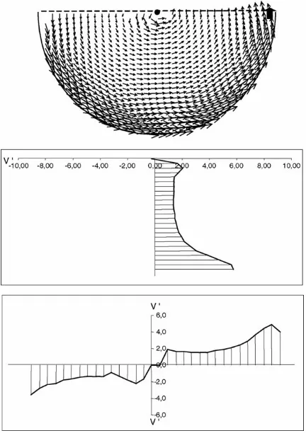
(37) 232. J. Oca et al. / Aquacultural Engineering 31 (2004) 221–236. Entry. Fig. 12. Field velocities in a horizontal section of one of the tank halves with configuration 4.. 3.4. Configuration 4: tangential inlets placed in the centre of the longer side wall This kind of configuration is made in order to force the formation of large eddies occupying the whole tank width. The outlets are placed in the centre of these eddies in a similar way to those in the mixed-cell rearing unit described by Watten et al. (2000). This can provide some of the advantages of the circular tanks described in Section 1 (uniformity and self-cleaning) while maintaining the operating advantages of rectangular tanks. The analysed configuration is probably the simplest way to induce this flow pattern with the minimal number of water inlets. In Fig. 12 we can see a single eddy occupying a half of the whole tank volume. The eddy shape was slightly elliptical, the largest diameter being 1.25 times the shortest. The time-stability of the flow pattern obtained, together with the absence of relevant vertical gradient of velocities, must be highlighted. One of the advantages of this configuration is the higher velocities achieved, preventing the biosolids from settling on the tank bottom. The ratio between the average measured velocity in the horizontal section (vavg ) and the expected average velocity assuming plug flow conditions (vpf : recirculation flow rate divided by water depth and tank width), will give a measure of the velocity increase obtained with this configuration. In the present case, the measured average velocity in the horizontal section was 2.88 cm s−1 , which is around 12 times the plug flow velocity, much higher than those obtained with the previous configurations. The ratio between the average velocity and the inlet jet velocity in this experiment was 0.037, lower than the 0.2 reported for circular tank designs (Skybakmoen, 1989), but very close to the percent obtained by Watten et al. (2000) in a rectangular tank with six horizontal eddies with a diameter about six times larger. These ratios can be increased optimising the water inlet velocity and the number and emplacement of the water inlets, or modifying slightly the tank geometry. This matter is the object of an ongoing new work..

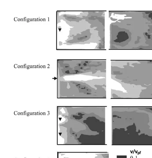
(38) J. Oca et al. / Aquacultural Engineering 31 (2004) 221–236. 233. Fig. 13. Spatial distribution of the non-dimensional velocity (v/vpf ) in the horizontal section of the four analysed configurations.. 3.5. Comparison between configurations Water velocity is a parameter strongly influencing the performance of a tank for fish culture, through both its self-cleaning function and the fish energy expenditure caused by swimming. To illustrate the differences between the ranges of velocities obtained with all the configurations analysed and their spatial distribution Fig. 13 has been designed. It shows the tank area occupied by the different ranges of velocities in a horizontal section, at a depth of around a 1/4 the water depth. The higher settlement of biosolids is expected in areas with lower velocities. To make the comparison between configurations easier, velocities have been given in a non-dimensional way, relating the velocity at every point with vpf and giving, in all the figures, the distribution of the ratio v/vpf in the horizontal section. In configuration 4, velocities are higher than 10 times vpf in 70% of the tank area and higher than five times vpf in 94% (Table 2). This means that it is easier to prevent the sedimentation of biosolids inside the tank, a downstream water treatment being necessary to collect them. In this configuration, the swimming performance of fish using this tank could be better than in a typical plug flow tank, considering that forced swimming improves fish growth and disease resistance as cited by Watten et al. (2000). Furthermore, water velocity can be accurately controlled in this tank, and it can be adapted to the requirements of several species, sizes, ages or culture situations..

(39) 234. J. Oca et al. / Aquacultural Engineering 31 (2004) 221–236. Table 2 Percentage of the tank area with v/vpf included in the intervals 0–1, 2–5, 5–10 and larger than 10, and average of v/vpf in the whole tank v/vpf. vavg /vpf. 0–1. 1–2. 2–5. 5–10. >10. Configuration 1 First half Second half Whole. 2.18 13.72 7.95. 11.51 34.59 23.05. 27.38 46.92 37.15. 32.94 4.77 18.85. 25.99 0.00 13.00. 7.06 2.25 4.68. Configuration 2 First half Second half Whole. 6.94 1.59 4.27. 19.44 10.71 15.08. 46.23 52.98 49.60. 17.86 27.98 22.92. 9.52 6.75 8.13. 4.55 4.69 4.62. Configuration 3 First half Second half Whole. 33.40 42.06 37.73. 18.69 41.27 29.98. 32.21 16.07 24.14. 10.14 0.60 5.37. 5.57 0.00 2.78. 2.94 1.21 2.08. Configuration 4 Whole. 1.14. 1.37. 3.42. 24.37. 69.70. 11.76. The second half of the tank in configuration 3 is the closest to the plug flow conditions, with 42% of the area below the vpf and 83% of the area below two times vpf . If the exchange rate or the fish density is not very high, we can expect most of the biosolids to settle inside the tank, having to be collected from the tank bottom, thus providing a very deficient self-cleaning function. Configurations 1 and 2 give the most heterogeneous distribution of velocities in the tank area, which will also produce a heterogeneous distribution of biosolids on the tank bottom. This sedimentation of biosolids does not exclude their presence in the effluent, due to the existence of internal streams attributable to the horizontal eddies formed all along the tank and also to the great penetration of the inlet plume in configuration 2. The heterogeneity inside the tank would have a direct effect on the use of the tank by fish. The higher the heterogeneity in water quality, the lesser the efficiency of the water use and space by fish. Furthermore, when strong gradients are set in the tank, territorial behaviour takes place, as Ross et al. (1995) demonstrated with rainbow trout maintained in plug-flow tanks, and as a consequence agonistic interactions arose between fish.. 4. Conclusions Particle tracking velocimetry has proved to be a very useful tool for three-dimensional study of the hydrodynamic characteristics of fish production tanks in a quick and inexpensive way. In rectangular tanks, these hydrodynamic characteristics have shown to be dramatically affected by the emplacement of the water inlets and by their geometry, providing big differences in mixing conditions and distribution of velocities inside the tank..

(40) J. Oca et al. / Aquacultural Engineering 31 (2004) 221–236. 235. The mixing between entering and remaining water was shown to be very low in configuration 2 (with a single horizontal entry) where considerable short-circuiting streams can be expected. Configurations with single or multiple waterfalls (configurations 1 and 3) showed a zone of intense mixing around the inlet occupying a semicircular area with a radius of around two and a half times the water depth in the single waterfall, and extending the whole tank width when the existence of multiple waterfalls allowed these areas to overlap. In configuration 4, with tangential inlets, the higher velocities obtained in the eddy will contribute to obtaining a good mixing and uniform environmental conditions in the entire tank volume. The appearance of dead volumes is especially significant in configurations with a single entry (configurations 1 and 2) in the centre of the horizontal eddies formed along the tank area. The emplacement of these dead volumes is mostly unpredictable, due to the time dependence on the flow patterns obtained with these configurations. Only in the configuration with multiple waterfalls (configuration 3), can the obtained flow pattern be considered to be close to the plug flow conditions, without the presence of horizontal eddies outside the area of intense mixing above described and in the area closer to the outlet. The distance between the inlets was shown to have an appreciable influence on the uniformity of the horizontal velocity field, which increased noticeably when the distance between inlets was reduced from 3.8 to 2.5 times the water depth. This increase in uniformity provides higher efficiency in water use. The distribution of velocity magnitude inside the tank is much more uniform in configuration 4, which has also the highest average velocities. These characteristics make this kind of configuration the most interesting for the achievement of self-cleaning conditions. Increases in the number of inlet points and modifications in the tank geometry could increase the average velocities, but the tank construction and the fish management could also become more complicated. Further trials are being developed to analyse the effect of some single modifications in the tank geometry using PTV techniques.. Acknowledgements This research was financed by the “Centre de Referència en Aqüicultura de la Generalitat de Catalunya”. Thanks are also due to Dr. Juan Ignacio Montero, researcher from the “Institut de Recerca i Tecnologia Agroalimentària” (IRTA) for its support in image processing.. References Burley, R., Klapsis, A., 1985. Flow distribution studies in fish rearing tanks. Part 2: Analysis of hydraulic performance of 1 m square tank. Aquacult. Eng. 4, 113–134. Burrows, R.E., Chenoweth, H.H., 1955. Evaluation of 3 types of rearing ponds. US Department of the Interior, Fish and Wildlife Service, Research Report, pp. 29–39. Chang, K.-A., Cowen, E.A., Liu, P.L.-F., 2002. Wave acceleration measurement using PTV technique. In: Piv and Modelling Water Wave Phenomena, An International Symposium in Cambridge, UK, 17–19 April 2002. Cripps, S.J., Poxton, M.G., 1992. A review of the design and performance of tanks relevant to flatfish culture. Aquacult. Eng. 11, 71–91. Cripps, S.J., Poxton, M.G., 1993. A method for the quantification and optimization of hydrodynamics in culture tanks. Aquacult. Int. 1, 55–71..