Empirical Essays on Monetary Policy

Texto completo

(1)Universitat Autònoma de Barcelona Departament d'Economia Aplicada. Empirical Essays on Monetary Policy. PhD Dissertation. by Bořek Vašíček. Supervisor: Prof. Luca Gambetti Departament d'Economia e Historia Economica Universitat Autònoma de Barcelona. Barcelona October 2010.

(2)

(3) Danečkovi.

(4)

(5) Acknowledgements I would like to express my gratitude to many people who made this dissertation possible. First, I wish to thank my family and friends (especially to all my colleagues from UAB: Ana, Chari, María, Helena, Guille, Javier, Ramón and many others) for their support that allowed me to finish this dissertation. My special thank is for my partner Inma for all those nice years together and for our little Daniel for the happiness that fulfilled my life on February 6, 2010 when he was born. I want to thank my supervisor Prof. Luca Gambetti for his guidance and suggestions during the dissertation research. I am very grateful to my co-authors Jaromír Baxa from Charles University, Prague and Roman Horváth from the Czech National Bank for an excellent collaboration and stimulating discussions over the last years. I have also benefited from comments made by Peter Clayes, Evi Pappa, Hugo Rodríguez and participants at seminars and conferences where I presented earlier versions of the papers forming this dissertation. The hospitality of the Department of Applied Economics, Universitat Autonoma de Barcelona as well as of Institute for Economic Analysis (CSIC), where most part of the research was conduced as well as financial support of Spanish Agency of International Cooperation (AECI) is gratefully acknowledged.. Barcelona, October 2010. Bořek Vašíček.

(6) ii.

(7) Contents. ii. List of Tables. iv. List of Figures. v. Introduction. 1. References………………………………………………..................................................... 8. Chapter 1. How Does Monetary Policy Change? Evidence on Inflation Targeting Countries. 11. 1.1 Introduction…………………………………………………………………………… 1.2 Related Literature……………………………………………………………………... 1.2.1 Monetary policy rules and inflation targeting…………………………………... 1.2.2 Time variance in monetary policy rules………………………………………… 1.3 Empirical Methodology................................................................................................. 1.3.1 The empirical model…………………..………………………………………... 1.3.2 The dataset….……………………………………............................................... 1.4 Results………………...………………………………………..………………..... 1.4.1 United Kingdom…………………………………………………………............ 1.4.2 New Zealand………………………………………….……………………........ 1.4.3 Australia………………………………………….………………………........... 1.4.4 Canada…………………………………………………………………………... 1.4.5 Sweden………………………………………….………………………………. 1.4.6 Inflation targeting and inflation persistence…………………………………….. 1.5 Concluding Remarks………………………………………………………………….. References………………………………………………………………………………… Appendix………………………………………………………………………………….. A.1.1 The VC Method………………………………………………………………… A.1.2 The Effects of Endogeneity in Policy Rules……………………………………. 11 13 13 15 19 19 25 26 26 30 32 34 36 38 41 42 46 47 50. Chapter 2. Monetary Policy Rules and Financial Stress: Does Financial Instability Matter for Monetary Policy?. 57. 2.1 Introduction…………………………………………………………………………… 2.2 Related Literature………………………………………………….………………….. 2.2.1 Monetary policy (rules) and financial instability – some theory.......................... 2.2.2 Monetary policy (rules) and financial instability – empirical evidence................ 2.2.3 Measures of financial stress.................................................................................. 2.3 Data and Empirical Methodology…………………………………………………….. 2.3.1 The dataset............................................................................................................ 2.3.2 The empirical model…………………………………………………………….. 57 58 58 61 62 64 64 68. iii.

(8) 2.4 Results………………………………………………………………………………… 2.5 Concluding Remarks…………………………………………………….……………. References………………………………………………………………………………… Appendix………………………………………………………………………………….. A.2.1 Time-varying Monetary Policy Rules………………………………………….. A.2.2 The Results with Interbank Rate as the Dependent Variable in the Policy Rule……………………………………………………………………………. A.2.3 The Results with Different Leads and Lags of the FSI………………………… A.2.4 The Results with Individual Variables of Bank Stress and Stock Market Stress.. 74 82 83 88 88. Chapter 3. Is Monetary Policy in New Members States Asymmetric?. 99. 3.1 Introduction…………………………………………………………………………… 3.2 Rationales for Asymmetric Monetary Policy…………………………………………. 3.3 Empirical Testing of Asymmetric Monetary Policy………………………………….. 3.3.1 Nonlinearities in the economic system…………………………………………. 3.3.2 Asymmetric preferences of the central bank……………………………………. 3.3.3 Policy regimes with a threshold effect………………………………………….. 3.4 Data Description……………………………………………………………………… 3.5 Empirical Results……………………………………………………………………... 3.5.1 Linear monetary policy rules…………………………………………………… 3.5.2 Nonlinear monetary policy rules due to nonlinearities in the economic system... 3.5.3 Nonlinear monetary policy rules due to asymmetric preferences………………. 3.5.4 Nonlinear monetary policy rules via threshold effects......................................... 3.6. Conclusions................................................................................................................... References............................................................................................................................ Appendix............................................................................................................................... 93 95 96. 99 101 102 104 104 106 109 110 110 111 114 117 123 124 127. Chapter 4. Inflation dynamics and the New Keynesian Phillips curve in 133 four Central European countries 4.1 Introduction…………………………………………………………………………… 4.2 The Theory and Empirics of the NKPC………………………………………………. 4.3 Econometric Approach……………………………………………………………….. 4.4 Data and Time Series Analysis………………………………………………….……. 4.4.1 Data description.................................................................................................... 4.4.2 Identification in forward-looking model............................................................... 4.4.3 Cross correlations……………………………………………………………….. 4.5 Empirical Results……………………………………………………………………... 4.5.1 Czech Republic…………………………………………………………………. 4.5.2 Hungary…………………………………………………………………………. 4.5.3 Poland…………………………………………………………………………… 4.5.4 Slovakia…………………………………………………………………………. 4.5.5 Discussion………………………………………………………………………. 4.6 Concluding Remarks………………………………………………………………….. References………………………………………………………………………………… Appendix………………………………………………………………………………….. iv. 133 135 140 143 143 144 145 146 146 149 150 152 153 155 157 161.

(9) List of Tables Chapter 1 Table A.1.1: Estimated coefficients of endogeneity correction terms……………………. 55. Chapter 3 Table 3.1: GMM estimates of the linear monetary policy rule…………………………… 111 Table 3.2: OLS/GARCH estimates of simple linear/non-linear Phillips curves)……….... 112 Table 3.3: GMM estimates of the nonlinear monetary policy rule I……………………… 113 Table 3.4: GMM estimates of the nonlinear monetary policy rule II…………………….. 115 Table 3.5: GMM estimates of the nonlinear monetary policy rule III……………………. 117 Table 3.6: 2SLS estimates of the FSI threshold value and GMM estimates of the monetary policy rule in each regime ……………………………………………………... 122 Chapter 4 Table 4.1: F-test of the necessary condition for identification in the forward-looking model……………………………………………………………………………………… 145 Table 4.2: Dynamic cross-correlations of the (log) real unit labor cost and the output gap with lags and leads of yearly HCPI inflation……………………………………………... 146 Table 4.3: GMM estimates of different versions of the closed economy PC and the PC augmented by external variables – the Czech Republic…………………………………... 148 Table 4.4: GMM estimates of different versions of the closed economy PC and the PC augmented by external variables – Hungary……………………………............................ 149 Table 4.5: GMM estimates of different versions of the closed economy PC and the PC augmented by external variables – Poland………………………………………………... 151 Table 4.6: GMM estimates of different versions of the closed economy PC and the PC augmented by external variables – Slovakia……………………………………………… 153. v.

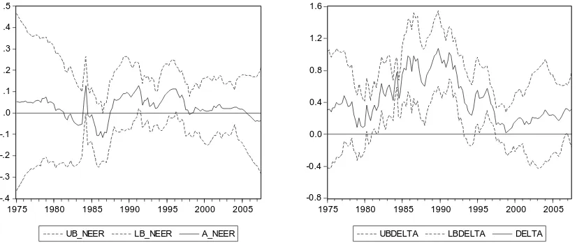
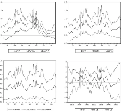
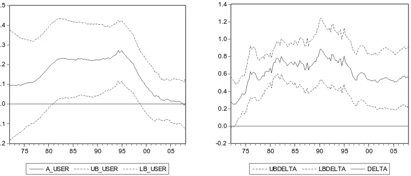
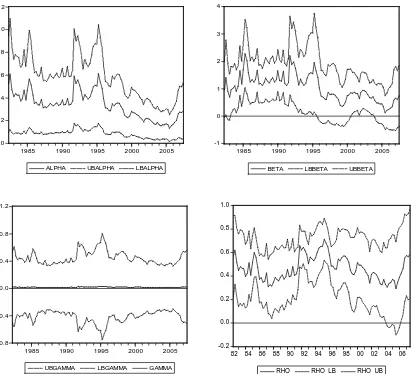
(10) List of Figures Chapter 1 Figure 1.1: Time-varying response coefficients in baseline (closed economy) policy rule, the UK…………………………………………………………………………………….. 28 Figure 1.2: Time-varying response coefficients in augmented (open economy) policy rule, the UK………………………………………………………………………………... 29. Figure 1.3: Time-varying response coefficients in baseline (closed economy) policy rule, New Zealand………………………………………………………………………………. 31. Figure 1.4: Time-varying response coefficients in baseline (closed economy) policy rule, New Zealand………………………………………………………………………………. 32. Figure 1.5: Time-varying response coefficients in baseline (closed economy) policy rule, Australia………………………………………………………………………………….... 33. Figure 1.6: Time-varying response coefficients in augmented (open economy) policy rule, Australia…………………………………………………………………………….... 34. Figure 1.7: Time-varying response coefficients in baseline (closed economy) policy rule, Canada……………………………………………………………………………………... 35. Figure 1.8: Time-varying response coefficients in augmented (open economy) policy rule, Canada……………………………………………………………………………….. 36. Figure 1.9: Time-varying response coefficients in baseline (closed economy) policy rule, Sweden…………………………………………………………………………………….. 37. Figure 1.10: Time-varying response coefficients in augmented (open economy) policy rule, Sweden……………………………………………………………………………….. 38. Figure 1.11: Time-varying response coefficients in AR(1) model for inflation…………... 40. Figure A.1.1: Time-varying response coefficients in baseline (closed economy) policy rule (with vs. without endogeneity correction), the UK………………………………….... 54. Figure A.1.2: Time-varying response coefficients in baseline (closed economy) policy rule (with vs. without endogeneity correction), New Zealand…………………………….. 55. Figure A.1.3: Time-varying response coefficients in baseline (closed economy) policy rule (with vs. witout endogeneity correction), Australia…………………………………... 56. Figure A.1.4: Time-varying response coefficients in baseline (closed economy) policy rule (with vs. without endogeneity correction), Canada ………………………………….. 57. Figure A.1.5: Time-varying response coefficients in baseline (closed economy) policy rule (with vs. without endogeneity correction), Sweden…………………………………... 58. vi.

(11) Chapter 2 Figure 2.1: IMF Financial stress index……………………………………………………. 67. Figure 2.2: The effect of financial stress on interest rate setting………………………….. 75. Figure 2.3: The effect of financial stress components on interest rate setting: bank stress, exchange rate stress and stock market stress………………………………………………. 79. Figure A.2.1.1: Time-varying monetary policy rules: the US…………....……………….. 88. Figure A.2.1.2: Time-varying monetary policy rules: the UK…………………………….. 89. Figure A.2.1.3: Time-varying monetary policy rules: Sweden ……………...……………. 90. Figure A.2.1.4: Time-varying monetary policy rules: Australia……………………...….... 91. Figure A.2.1.5: Time-varying monetary policy rules: Canada……………………...…….. 92. Figure A.2.2.1: The effect of financial stress on interest rate setting (interbank rate as the dependent variable)………………………………………………………………………... 93. Figure A.2.2.2: The effect of financial stress components on interest rate setting: bank stress, exchange rate stress and stock market stress (interbank rate as the dependent variable)………………………………………………………………………………….... 94. Figure A.2.3.1: The effect of financial Stress (t-1 vs. t-2, t, t+1, t+2) on Interest Rate Setting……………………………………………………………………………………... 95. Figure A.2.4.1: The effect of bank stress on interest rate setting………………...………... 96. Figure A.2.4.2: The effect of stock market stress on interest rate setting………………..... 97. Chapter 3 Figure 3.1: Scatter plots between smoothed inflation rate and output gap (the Phillips curve) and fitted linear trend……………………………………………………………… 113 Figure A.3.1: Proxies of inflation gap (inflation deviation from 1. the inflation HP trend, 2. the official target, 3. the official target HP trend)……………………………………… 127 Figure A.3.2: IMF Emerging-markets financial stress index (EM-FSI)………………….. 128 Figure A.3.3: Likelihood ratio sequence for different values of the threshold variable (the inflation gap)…………………………………………………………………………. 129 Figure A.3.4: Likelihood ratio sequence for different values of the threshold variable (the output gap)…………………………………………………………………………… 130 Figure A.3.5: Likelihood ratio sequence for different values of the threshold variable (the EM-FSI)……………………………………………………………………………… 131 vii.

(12) Chapter 4 Figure A.4.1: Yearly inflation rates and annualized quarterly inflation rates derived from HCPI (solid line) and GDP deflator………………………………………………………. 161 Figure A.4.2: Yearly rates HCPI inflation and inflation expectations 12 months ahead by financial markets – the Czech Republic and Poland……………………………………… 162. viii.

(13) Introduction This dissertation is divided into four essays, each of them having its own structure and methodological framework. Although each of the essays making the chapters of the thesis is self-contained, their topics are very closely related. Consequently, the reader will be able to follow the thesis in its unity.. The four essays are empirical and address some relevant issues from monetary economics and policy. In first three essays we aim at the way central banks sets their policy rates, which is usually described by central bank’s reaction function or a monetary policy rule (Taylor, 1993), and in the fourth one, we look at the inflation dynamics and the New Keynesian (NK) Phillips Curve (Galí and Gertler, 1999). In the first three papers, we look at different issues related to policy rules such as their nonlinearities, evolution across time, the intensity of interest rate response to inflation, degree of policy inertia as well as how policy changes when it is faced by financial stress.. The monetary policy rule and the NK Phillips Curve became key elements of the NK policy model (e.g. Galí, 2008), which is at present the most influential theoretic framework for analysis of macroeconomic dynamics and monetary policy both in academia and among monetary policy makers. Dynamics Stochastic General Equlibrium models (DSGE), which are the main analytic tools within most central banks (e.g. Area-Wide model of the European Central Bank), are inspired by the NK models. While the traditional Keynesian literature assumed sticky prices and wages in the short-term, it was unable to provide their satisfactory microeconomic explanations. The NK model enriched the original Keynesian literature by microeconomic foundations but at the same time by some important elements such as rational expectations and vertical long-term Phillips curve incompatible with the Keynesian tradition. Price rigidities (both nominal and real), which are result of imperfect competition, enable that monetary policy has impact on real variables in the short term. Such view on monetary policy is quite paradoxically close to monetarism but quite distant from other current macroeconomic branches such as Real Business Cycle Theory or Post-Keynesianism that cast doubt on the ability of monetary policy to affect real economy (Snowdon and Vane, 2005). In spite of the popularity of NK models, the empirical evidence goes behind the theory. The purpose of this thesis is to contribute to the empirics of the NK model.. 1.

(14) In each chapter we look at several countries in order to pursue comparative analysis. The reason for this choice is my conviction that empirical macroeconomic analysis can provide reliable results only when one is not limited by data of a particular country and period. Consequently, a comparative study faces a trade-off between the choice of model, method and data that are the most suitable for a particular country, on one hand, and the need to take homogeneous stance that allows comparison of the results, on the other. Cross-country analysis also forces the author to avoid subtle methodological adjustments to achieve “the best” or the most interesting results for a particular country. Given that the thesis is empirical, the methodology of each essay consists in use of a given macroeconomic model, specification of empirical relation that will become subject of analysis, selection of corresponding time series and an application of suitable econometric methods. In general, we look at two kinds of countries: (i) developed economies such as the US or the UK where not only monetary policy has a long-term tradition but also the data are of good quality and the time series cover several decades and (ii) post-transitional economies of new Central-European EU member states where the period for reasonable econometric analysis is substantially limited both by the process of economic transition itself but also by the data availability.. Chapter 1, How Does Monetary Policy Change? Evidence on Inflation Targeting Countries is a joint work with J. Baxa and R. Horváth. It examines how the monetary policy setting evolves in time. We aim at a group of inflation targeting (IT) countries (Australia, Canada, New Zealand, Sweden and the United Kingdom) because it seems especially interesting how the de-facto interest rate setting changes once this policy framework is introduced as well as whether the operative monetary policy under this regime is driven by some rule or is rather discretional.. The IT regime gained popularity as a monetary policy framework World and numerous academic studies suggest the gradual convergence of the inflation rate to its target as an optimal monetary policy (Clarida et al., 1999, 2000; Batini and Haldane, 1999). The IT feasibility has been confirmed by the experience of many countries that adopted this framework. However, there is still ongoing discussion what part of the decrease of inflation rate can be attributed to IT and the empirical evidence about the effect of this regime on other variables is mixed. Bernanke et al. (1999) assert that IT does not decrease the cost of disinflation and does not bring credibility to monetary policy immediately. The inflation expectations decrease only gradually over time. Ball (1999) concludes that IT is an efficient 2.

(15) policy with respect to inflation and output variance, but it is not superior to simple interestrate rules. Ball and Sheridan (2003) find that while the economic performance (inflation, output and interest rate variability) improved over time in OECD countries, there is no significant difference between countries pursuing IT and those using other policy arrangements. Moreno and Rey (2006) studying the inflation dynamics in various European countries found that IT had positive impact on the decrease of low frequency dynamic (inflation trend) because it decreases the size of monetary shocks.. In terms of discussion whether IT is rule-based or discretional, it is interesting to recall Bernanke’s claim (2003) that most major central banks in fact use constrained discretion. The word “constrained” reflects situation when central banks have explicit commitment of keeping the inflation low and stable. “Discretion” does not consist only in the freedom to choose the operative policy for achievement of the price stability but also conditioned on the fulfillment of the previous objective, the central bank can pursue other targets, in particular cycle stabilization. Svensson (2003) adverts to certain inconsistency between the need to follow policy rule from the commitment perspective and the recommendation not to apply the simple rules mechanically when no specification is provided what is the permitted deviation from the rule.. To examine the change in monetary policy rules across time, we use time-varying parameter model with endogenous regressors with aim to reveal if and how the interest rate setting changed as a consequence of adoption of IT regime without imposing ex-ante any structural breaks. To estimate this model we use novel moment-based estimator (Schlicht and Ludsteck, 2006) that has some desirable computational properties over the common Kalman filter.. The findings of this chapter can be resumed as follows. First, monetary policy rules change rather gradually than abruptly, which points to the importance of applying time-varying estimation models as opposed to switching models. Second, the interest rate smoothing parameter is much lower than what previous time-invariant estimates report. Therefore, the puzzle of high policy inertia found in many empirical studies, which is inconsistent with practical unpredictability of interest rate changes in middle-term (Rudebusch, 2006), seems to be driven by omission of time-variance of response coefficients. Third, the external factors matter most IT countries, albeit the importance of exchange rate diminishes after the IT adoption. Fourth, the response of interest rates to inflation is particularly strong during the 3.

(16) periods when central bankers want to break the record of high inflation such as in the U.K. at the beginning of 1980s. Contrary to common wisdom, the response becomes less aggressive after the IT adoption suggesting the positive effect of this regime on anchoring inflation expectations. This result is supported by our complementary finding that inflation persistence as well as policy neutral rate typically decreased after the adoption of inflation targeting.. Chapter 2, Monetary Policy Rules and Financial Stress:Does Financial Instability Matter for Monetary Policy? is a joint work with J. Baxa and R. Horváth. It extends the previous chapter examining whether and how main central banks (Australia, Canada, Sweden, the United Kingdom and the US) responded to the episodes of financial stress over the last three decades. Given that the interest rate response to financial stress must be nonlinear and only temporal, the time-varying coefficient model again seems to be the most suitable framework. This methodology accompanied by new financial stress dataset developed by the International Monetary Fund (IMF) allows not only testing whether the central banks responded to financial stress at all but also detecting the periods and type of stress that were for monetary authorities the most worrying.. The financial frictions such as unequal access to credits or debt collateralization were recognized to have important consequences for the transmission of monetary policy as they increase the response of aggregate demand to interest rate changes. Already Fisher (1933) presented the idea that adverse credit-market conditions can cause significant macroeconomic disequilibria. Kiyotaki and Moore (1997) showed that the credit markets are characterized by asymmetric information and principal-agent relationships when the durable assets are not only used in production process but they are often used as collateral for loans. The role of credit market frictions was incorporated to NK model by Bernanke et al. (1999). Their “financial accelerator” mechanism consists in the relation between net worth of borrows and the finance premium they have to pay. This relationship makes that any shock affecting the net worth of borrowers has accelerated affects on aggregate demand and output.. In spite of the potential effects the financial distress can have on real economy, the relation between monetary policy stance and financial stability is not straightforward. The financial stability is mainly not an explicit objective of monetary policy but it is rather retained by separate supervisory function of central banks. Although many DSGE models already include financial sector and model potential financial frictions (Tovar, 2009), the issues of viability to 4.

(17) modify monetary policy stance in face of financial stress (Cúrdia and Woodford, 2010) in general, or asset price misalignments in particular (Bernanke and Getler, 1999) are still subject to debate. Moreover, there are other puzzles such as how to measure the financial stress or whether the central banks in reality adjust the policy rates when financial markets are fragile (Borio and Lowe, 2004; Ceccheti and Li, 2008).. The IMF financial stress index (Cardarelli et al., 2009) is a comprehensive stress measure that tracks the overall financial stress alike the distress in different markets (banking sector, stock market and exchange rate market). Combined with time-varying model, we aim to quantify the intensity of the interest rate response to the financial stress. Our findings suggest that central banks usually loosen monetary policy in the face of high financial stress. We argue that all central banks kept its policy rates during the crisis by about 50 basis points on average (250 pb in case of the Bank of England) lower solely due to their response to financial stress (besides the decrease justified by developments in inflation expectations or the output gap). The current global turmoil stands out as an exceptional period both in term of the intensity of the response but also its coincidence for different central banks. There is a certain crosscountry and time heterogeneity when we look at central banks’ considerations of specific types of financial stress. While most central banks seem to respond to stock market stress and bank stress, exchange rate stress is found to drive the reaction of central banks only in more open economies.. Chapter 3, Is Monetary Policy in New Member States Asymmetric? extends the analysis of policy rules towards emerging market economies. In particular, we deal with potential asymmetries in monetary policy conduct of three new EU members (the Czech Republic, Hungary and Poland) that apply inflation targeting that is prone to policy asymmetries.. The empirical studies usually assume that monetary policy responds symmetrically to economic developments, in other words the monetary policy rule is modeled as a linear function. A theoretical underpinning of a linear policy rule is the common linear-quadratic (LQ) representation of macroeconomic models (economic structure is assumed to be linear and the policy objectives to be symmetric, in particular the loss function is quadratic). However, when the assumptions of the LQ framework are relaxed, the optimal monetary policy can be asymmetric, which can be represented by a nonlinear monetary policy rule. For example, a convex Phillips curve implies that the inflationary effects of excess demand are 5.

(18) larger than the disinflationary effects of excess supply (e.g. Laxton et al., 1999). Such situation can lead optimizing central bankers to behave asymmetrically (Dolado et al., 2005). On the other hand, asymmetric monetary policy can be related by asymmetric preferences of central bankers. For example, reputation reasons can drive central banks, especially those pursuing inflation-targeting, having an anti-inflation bias and respond more severely when inflation is high or exceeds its target value (Ruge-Murcia, 2004).. To test whether the monetary policy can be described in the three new EU member states as asymmetric, we apply two different empirical frameworks: (i) GMM estimation of models that allow discriminating between the sources of policy asymmetry but are conditioned by specific underlying relations (Dolado et al., 2005: Surico, 2007); and (ii) a flexible framework of sample splitting where nonlinearity enters via threshold variables and monetary policy is allowed to switch between regimes (Hansen, 2000; Caner and Hansen, 2004).. We find little evidence in favor of nonlinearities in economic system, in particular convexity of AS schedule, and therefore no reason for asymmetric policy. On the other hand, there is some evidence of asymmetric policy driven by central bank preferences in terms of inflation rate and the level of interest rate. Unfortunately, the validity of empirical results is conditioned by specific parametric models underlying the estimated nonlinear equations. Therefore, we use as an alternative a method of sample splitting where nonlinearities enter via a threshold variable and monetary policy is allowed to switch between two regimes. Besides the inflation and output gaps we used a financial stress index as competing threshold variables. The threshold effects are most evident with financial stress index. While the Czech and Polish National Banks seem to face the financial stress by decreasing their policy rates, the opposite pattern is found in Hungary.. Chapter 4, Inflation dynamics and the New Keynesian Phillips curve in Central European countries seeks to shed light on the inflation dynamics of four new EU members (Czech Republic, Hungary, Poland and Slovakia) and test whether the predominant theoretical model of inflation, the New Keynesian Philips Curve (NKPC), finds support in the data of these countries.. Understanding the nature of the inflation dynamics is very important for the implementation of monetary policy. Unlike the traditional PC that was a purely empirical model, the NKPC, 6.

(19) which appeared in the 1990’s, stands on elaborated micro-foundations of monopolistic competition and price rigidities (Taylor, 1980; Calvo, 1983). The NKPC links the current price inflation to inflation expectations of economic agents. However, as the data suggest that inflation is persistent process, several attempts were made to give inflation persistence some structural base (Galí and Gertler, 1999; Christiano et al., 2005). The current discussion on the inflation dynamics in general and the NKPC in particular aims at two main issues: (i) whether inflation is mainly backward-looking or forward-looking phenomenon and (ii) what is the principal inflation-forcing variable in the short-term. These characteristics of inflation have important consequences for monetary policy. In particular, if inflation is predominantly forward-looking phenomenon and its dependence on the past (intrinsic persistence) is limited, a credible monetary policy can achieve disinflation at no cost (in terms of real output loss).. Inflation in the NMS has some specific features as compared to developed countries. During most of the 1990s it has been affected by price liberalization. Therefore, inflation rates have been comparatively higher. Moreover, all four countries are small open economies and it is arguable that domestic price developments are influenced by external sources that were practically ignored in original empirical studies on the NKPC (Batini et al., 2005).. This chapter estimates both forward-looking and hybrid NKPC using different alternative forcing variables both domestic (the output gap, unit labor cost) and external (exchange rate, oil prices, foreign inflation rates). Besides assuming rational expectations in GMM framework (Galí and Gertler, 1999), we use survey data on inflation expectations where available (Zhang et al., 2009). Our main results can be resumed as follows. (1) The inflation rates in the four countries hold significant forward-looking component and therefore the current inflation is (at least partially) determined by its future expected value. However, the size and significance of the backward-looking terms suggest that inflation rates in the NMS are rather persistent. (2) The evidence in favor of the real marginal cost as the main inflation-forcing variable is fragile. The output gap performs better only marginally. On the other hand, we find some evidence that the short-term inflation impulses in the NMS can be external (oil prices, exchange rate, inflation rates abroad). (3) Inflation persistence of the NMS implies that antiinflationist policy could be accompanied by an output loss. The structural model behind the NKPC suggests that the effect of monetary policy on inflation goes via the marginal cost. However, if the marginal cost does affect inflation, monetary policy can influence inflation only via its credibility and its effect on inflation expectations. 7.

(20) References Ball, L. (1999): Efficient Monetary Policy Rules. International Finance 2:1, 63-83. Ball, L. and N. Sheridan (2003): Does Inflation Targeting Matter? NBER Working Paper, No. 9577. Batini, N. and A.G. Haldane (1999): Forward-Looking Rules for Monetary Policy. In: J. Taylor (ed.): Monetary Policy Rules University of Chicago Press for NBER, Cambridge. Batini, N., Jackson, B. and S.Nickell (2005): An Open-economy New Keynesian Phillips Curve for the U.K. Journal of Monetary Economics 52, 1061-1071. Bernanke, B. (2003): Constrained Discretion and Monetary Policy. Remarks before the Money Marketers of New York University, New York, February 3, 2003. Bernanke, B. and M. Gertler (1999): “Monetary Policy and Asset Price Volatility.” Economic Review (FRB of Kansas City), 17-51. Bernanke, B., Gertler, M. and S. Gilchrist (1999): The Financial Accelerator in a Quantitative Business Cycle Framework. In: J.B. Taylor, M. Woodford (eds): Handbook of Macroeconomics. North-Holland: Amsterdam. Bernanke, B.S., Laubach, T, Mishkin, F. and A.S. Posen (1999): Inflation Targeting: Lessons from the International Experience. Princeton University Press: Princeton. Borio, C. and P. Lowe (2004): Securing Sustainable Price Stability: Should Credit Come Back from the Wilderness? BIS Working Papers, No. 157. Calvo,G. (1983): Staggered Prices in a Utility Maximizing Framework. Journal of Monetary Economics 12, 383398. Caner, M and B.E. Hansen (2004): Instrumental Variables Estimation of a Threshold Model. Econometric Theory 20, 2004, 813-843. Cardarelli, R., S. Elekdag and S. Lall (2009): Financial Stress, Downturns, and Recoveries. IMF Working Paper, No. 09/100. Cecchetti, S. and L. Li (2008): Do Capital Adequacy Requirements Matter for Monetary Policy? Economic Inquiry 46(4), 643-659. Dolado, J.J., Maria-Dolores, R and F.J. Ruge-Murcia (2005): Are Monetary-policy Reaction Functions Asymmetric? The Role of Nonlinearity in the Phillips Curve. European Economic Review 49, 485-503. Clarida, R., Galí, J. and M. Gertler (1998): Monetary Policy Rules in Practice: Some International Evidence. European Economic Review 42, 1033-1067. Christiano, L.J., Eichenbaum, M. and Ch.L. Evans (2005): Nominal Rigidities and the Dynamic Effects of a Shock to Monetary Policy. Journal of Political Economy 113: 1-45. Clarida, R., Galí, J. and M. Gertler (1999): The Science of Monetary Policy: A New Keynesian Perspective. Journal of Economic Literature 37(4), 1661-1707. Clarida, R., Galí, J. and M. Gertler (2000): Monetary Policy Rules and Macroeconomic Stability. The Quarterly Journal of Economics 115(1), 147-180. Clarida, R., Galí, J. and M. Gertler (2003): Optimal Monetary Policy Rules in Open versus Closed Economies: An Integrated Approach. The American Economic Review 91(2), 248-252. Cúrdia, V. and M. Woodford (2010): Credit Spreads and Monetary Policy. Journal of Money, Credit and Banking 42, 3-35.. 8.

(21) Fisher, I. (1933): Debt-deflation Theory of Great Depressions. Econometrica 1(4), 337-357. Galí, J. and M. Gertler (1999): Inflation dynamics: A structural econometric analysis. Journal of Monetary Economics 44, 195-222. Galí, J. (2002): New Perspectives on Monetary Policy, Inflation, and the Business Cycle. NBER Working Paper, No. 8767. Galí, J. (2008): Monetary Policy, Inflation, and the Business Cycle. Princeton University Press: Princeton. Galí, J. and M. Gertler (1999): Inflation dynamics: A structural econometric analysis. Journal of Monetary Economics 44, 195-222. Hansen, B.E. (2000): Sample Splitting and Threshold Estimation. Econometrica 68, 575- 603. Laxton, D., Rose, D. and D. Tambakis (1999): The U.S. Phillips Curve: The Case for Asymmetry. Journal of Economic Dynamics and Control 23 (9-10): 1459-1485. Kiyotaki, N. and J. Moore (1997): Credit Cycles. The Journal of Political Economy 105, 211-248. Moreno, A. and L. Rey (2006): Inflation Targeting in Western Europe. Topics in Macroeconomics, Vol. 6, Issue 2, Article 6. Rudebusch, G. (2006): Monetary Policy Inertia: Fact or Fiction? International Journal of Central Banking 2(4), 85-136. Ruge-Murcia, F.J. (2004): The Inflation Bias when the Central Banker Targets the Natural Rate of Unemployment. European Economic Review 48, 91-107. Schlicht, E. and J.Ludteck (2006): Variance Estimation in a Random Coefficients Model, IZA Discussion paper No. 2031. Snowdon, B. and H.R. Vane (2005): Modern Macroeconomics: Its Origin, Development and Current State. Edwar Adgar Publishing: Northampton, Massachusetts. Surico, P. (2007): The Monetary Policy of the European Central Bank. Scandinavian Journal of Economics 109(1), 115-135. Taylor, J.B. (1980): Aggregate Dynamics and Staggered Contracts. Journal of Political Economy 88, 1-23. Taylor, J.B. (1993): Discretion versus Policy Rules in Practice. Carnegie-Rochester Conference Series on Public Policy 39, 195-214. Tovar, C. E. (2009): DSGE Models and Central Banks. Economics: The Open-Access, Open-Assessment EJournal 3, 2009-16. Zhang, Ch., Osborn, D.R. and D.H. Kim (2009): Observed Inflation Forecasts and the New Keynesian Phillips Curve. Oxford Bulletin of Economics and Statistics 71, 375-398.. 9.

(22) 10.

(23) Chapter 1. How Does Monetary Policy Change? Evidence on Inflation Targeting Countries 1.1 Introduction Taylor-type regressions have been applied extensively in order to describe monetary policy setting for many countries. The research on U.S. monetary policy usually assumes that monetary policy was subject to structural breaks when the Fed chairman changed. Clarida et al. (2000) claim that the U.S. inflation during the 1970s was unleashed because the Fed’s interest rate response to the inflation upsurge was too weak, while the increase of such response in the 1980s was behind the inflation moderation. Although there is ongoing discussion on the sources of this Great Moderation (Benati and Surico, 2009), it is generally accepted that monetary policy setting evolves over time.. The evolution of monetary policy setting as well as exogenous changes in the economic system over time raises several issues for empirical analysis. In particular, the coefficients of monetary policy rules estimated over longer periods are structurally unstable. The solution used in the literature is typically sub-sample analysis (Clarida et al., 1998, 2000). Such an approach is based on the rather strong assumption that the timing of structural breaks is known, but also that policy setting does not evolve within each sub-period. Consequently, this gives impetus to applying an empirical framework that allows for regime changes or, in other words, time variance in the model parameters (Cogley and Sargent, 2001, 2005). Countries that have implemented the inflation targeting (IT) regime are especially suitable for such analysis because it is likely that the monetary policy stance with respect to inflation and other macroeconomic variables changed as a consequence of the implementation of IT. Moreover, there is ongoing debate of to what extent IT represents a rule-based policy. Bernanke et al. (1999) claim that IT is a framework or constrained discretion rather than a mechanical rule. Consequently, the monetary policy rule of an IT central bank is likely to be time varying.. Our study aims to investigate the evolution of monetary policy for countries that have long experience with the IT regime. In particular, we analyze the time-varying monetary policy rules for Australia, Canada, New Zealand, Sweden and the United Kingdom. As we are. 11.

(24) interested in monetary policy evolution over a relatively long period, we do not consider countries where IT has been in place for a relatively short time (Finland, Spain), or was introduced relatively recently (such as Armenia, the Czech Republic, Hungary, Korea, Norway and South Africa). We apply the recently developed time-varying parameter model with endogenous regressors (Kim and Nelson, 2006), as this technique allows us to evaluate changes in policy rules over time, and, unlike Markov-switching methods, does not impose sudden policy switches between different regimes. On top of that, it also deals with endogeneity of policy rules. Unlike Kim and Nelson (2006) we do not rely on the Kalman filter, which is conventionally employed to estimate time-varying models, but employ the moment-based estimator proposed by Schlicht and Ludsteck (2006)1 for its mathematical and descriptive transparency and minimal requirements as regards initial conditions. In addition, Kim and Nelson (2006) apply their estimator to evaluate changes in U.S. monetary policy, while we focus on inflation targeting economies.. Anticipating our results, we find that monetary policy changes gradually, pointing to the importance of applying a time-varying estimation framework (see also Koop et al., 2009, on evidence that monetary policy changes gradually rather than abruptly). When the issue of endogeneity in time-varying monetary policy rules is neglected, the parameters are estimated inconsistently, even though the resulting errors are economically not large. Second, the interest rate smoothing parameter is much lower than typically reported by previous timeinvariant estimates of policy rules. This is in line with a recent critique by Rudebusch (2006), who emphasizes that the degree of smoothing is rather low. External factors matter for understanding the interest rate setting process for all countries, although the importance of the exchange rate diminishes after the adoption of inflation targeting. Third, the response of interest rates to inflation is particularly strong during periods when central bankers want to break a record of high inflation, such as in the UK at the beginning of the 1980s. Contrary to common wisdom, the response can become less aggressive after the adoption of inflation targeting, suggesting a positive anchoring effect of this regime on inflation expectations or a low inflation environment. This result is consistent with Kuttner and Posen (1999) and Sekine and Teranishi (2008), who show that inflation targeting can be associated with a smaller. 1. The description of this estimator is also available in Schlicht (2005), but we refer to the more recent working paper version, where this estimator is described in a great detail. Several important parts of this framework were introduced already in Schlicht (1981). 12.

(25) response of the interest rate to inflation developments if the previous inflation record was favorable.. The paper is organized as follows. Section 2 discusses the related literature. Section 3 describes our data and empirical methodology. Section 4 presents the results. Section 5 concludes. An appendix with a detailed description of the methodology and additional results follows.. 1.2 Related Literature 1.2.1 Monetary policy rules and inflation targeting Although the theoretical literature on optimal monetary policy usually distinguishes between instrument rules (the Taylor rule) and targeting rules (the inflation-targeting based rule), the forward-looking specification of the Taylor rule, sometimes augmented with other variables, has commonly been used for the analysis of decision making of IT central banks. The existing studies feature great diversity of empirical frameworks, which makes the comparison of their results sometimes complicated. In the following we provide a selective survey of empirical studies aimed at the countries that we focus on.. The United Kingdom adopted IT in 1992 (currently a 2% target and a ±1% tolerance band) and the policy of the Bank of England (BoE) is subject to the most extensive empirical research. Clarida et al. (1998) analyzed the monetary policy setting of the BoE in the pre-IT period, concluding that it was consistent with the Taylor rule, yet additionally constrained by foreign (German) interest rate setting. Adam et al. (2005) find by means of sub-sample analysis that the introduction of IT did not represent a major change in monetary policy conduct, unlike the granting of instrument independence in 1997. Taylor and Davradakis (2006) point to significant asymmetry of British monetary policy during the IT period; in particular the BoE was concerned with inflation only when it significantly exceeded its target. Assenmacher-Wesche (2006) concludes by means of a Markov-switching model that no attention was paid to inflation until IT was adopted. Conversely, Kishor (2008) finds that the response to inflation had already increased, especially after Margaret Thatcher became prime minister (in 1979). Finally, Trecroci and Vassalli (2009) use a model with time-varying. 13.

(26) coefficients and conclude that policy had been getting gradually more inflation averse since the early 1980s.. New Zealand was the first country to adopt IT (in 1990). A particular feature besides the announcement of the inflation target (currently a band of 1–3%) is that the governor of the Reserve Bank (RBNZ) has an explicit agreement with the government. Huang et al. (2001) study the monetary policy rule over the first decade of IT. He finds that the policy of the RBNZ was clearly aimed at the inflation target and did not respond to output fluctuations explicitly. The response to inflation was symmetric and a backward-looking rule does as good a job as a forward-looking one at tracking the interest rate dynamics. Plantier and Scrimgeour (2002) allow for the possibility that the neutral real interest rate (implicitly assumed in the Taylor rule to be constant) changes in time. In this framework they find that the response to inflation increased after IT was implemented and the policy neutral interest rate tailed away. Ftiti (2008) additionally confirms that the RBNZ did not explicitly respond to exchange rate fluctuations and Karedekikli and Lees (2007) disregard asymmetries in the RBNZ policy rule.. The Reserve Bank of Australia (RBA) turned to IT in 1993 (with a target of 2–3%) after decades of exchange rate pegs (till 1984) and consecutive monetary targeting.2 De Brouwer and Gilbert (2005) using sub-sample analysis confirm that the RBA’s consideration of inflation was very low in the pre-IT period and a concern for output stabilization was clearly predominant. The response to inflation (both actual and expected) increased substantially after IT adoption but the RBA seemed to consider exchange rate and foreign interest rate developments as well. Leu and Sheen (2006) find a lot of discretionality in the RBA’s policy (a low fit of the time-invariant rule) in the pre-IT period, a consistent response to inflation during IT, and signs of asymmetry in both periods. Karedekikli and Lees (2007) document that the policy asymmetry is related to the RBA’s distaste for negative output gaps.. The Bank of Canada (BoC) introduced IT in 1991 in the form of a series of targets for reducing inflation to the midpoint of the range of 1–3% by the end of 1995 (since then the target has remained unchanged). Demers and Rodríguez (2002) find that the implementation of this framework was distinguished by a higher inflation response, but the increase in the 2. In Australia, the adoption of inflation targeting was a gradual process. As from January 1990, the RBA increased the frequency of its communications via speeches and the style of the Bank’s Bulletin started to correspond to the inflation reports as introduced in New Zealand. The exact inflation target was defined explicitly later, in April 1993. Greenville (1997) describes the policy changes in Australia in great detail. 14.

(27) response to real economic activity was even more significant. Shih and Giles (2009) model the duration analysis of BoC interest rate changes with respect to different macroeconomic variables. They find that annual core inflation and the monthly growth rate of real GDP drive the changes of the policy rate, while the unemployment rate and the exchange rate do not. On the contrary, Dong (2008) confirms that the BoC considers real exchange rate movements.. Sweden adopted IT in 1993 (a 2% target with a tolerance band of 1 percentage point) just after the krona had been allowed to float. The independence of Sveriges Riksbank (SR) was legally increased in 1999. Jansson and Vredin (2003) studied its policy rule, concluding that the inflation forecast (published by the Riksbank) is the only relevant variable driving interest rate changes. Kuttner (2004) additionally finds a role for the output gap, but in terms of its growth forecast (rather than its observed value). Berg et al. (2004) provide a rigorous analysis of the sources of deviations between the SR policy rate and the targets implied by diverse empirical rules. They claim that higher inflation forecasts at the early stages of the IT regime (due to a lack of credibility) generate a higher implied target from the forward-looking rule and therefore induce spurious indications of policy shocks. Their qualitative analysis of SR documents clarifies the rationale behind actual policy shocks, such as more gradualism (stronger inertia) in periods of macroeconomic uncertainty.. Finally, there are a few multi-country studies. Meirelles Aurelio (2005) analyzes the timeinvariant rules of the same countries as us, finding significant dependence of the results on real-time versus historical measures of variables. Lubik and Schorfheide (2007) estimate by Bayesian methods an open economy structural model of four IT countries (AUS, CAN, NZ, UK) with the aim of seeing whether IT central banks respond to exchange rate movements. They confirm this claim for the BoE and BoC. Dong (2008) enriches their setting by incorporating some more realistic assumptions (exchange rate endogeneity, incomplete exchange-rate pass-through), finding additionally a response to the exchange rate for the RBA.. 1.2.2 Time variance in monetary policy rules The original empirical research on monetary policy rules used a linear specification with timeinvariant coefficients. Instrument variable estimators such as the GMM gained popularity in this context, because they are able to deal with the issue of endogeneity that arises in the. 15.

(28) forward-looking specification (Clarida et al., 1998).3 While a time-invariant policy rule may be a reasonable approximation when the analyzed period is short, structural stability usually fails over longer periods.. The simplest empirical strategy for taking time variance into account is to use sub-sample analysis (Taylor, 1999; Clarida et al., 2000). The drawback of this approach is its rather subjective assumptions about points of structural change and structural stability within each sub-period. An alternative is to apply an econometric model that allows time variance for the coefficients. There are various methods dealing with time variance in the context of estimated monetary policy rules.. The most common option is the Markov-switching VAR method, originally used for business cycle analysis. Valente (2003) employs such a model with switches in the constant term representing the evolution of the inflation target (the inflation target together with the real equilibrium interest rate makes the constant term in a simple Taylor rule). AssenmacherWesche (2006) uses the Markov-switching model with shifts both in the coefficients and in the residual variances. Such separation between the evolution of policy preferences (coefficients) and exogenous changes in the economic system (residuals) is important for the continuing discussion on the sources of the Great Moderation (Benati and Surico, 2009; Canova and Gambetti, 2008). Sims and Zha (2006) present a multivariate model with discrete breaks in both coefficients and disturbances. Unlike Assenmacher-Wesche they find that the variance of the shock rather than the time variance of the monetary policy rule coefficient has shaped macroeconomic developments in the U.S. in the last four decades.. The application of Markov-switching VAR techniques turns out to be complicated for IT countries, where the policy rules are usually characterized as forward-looking and some regressors become endogenous. The endogeneity bias can be avoided by means of a backward-looking specification (lagged explanatory variables), but this is very probably inappropriate for IT central banks, which are arguably forward-looking.4 However, there is another distinct feature of the Markov-switching model that makes its use for the analysis of 3. One exception is when a researcher uses real-time central bank forecasts for Taylor-type rule estimation, i.e. the data available to the central bank before the monetary policy meeting. In such case, the endogeneity problem will not arise and least squares estimation may perform well (Orphanides, 2001). However, as we will discuss in more detail below, the use of real-time data may not solve the issue of endogeneity completely. 4 Psaradakis et al. (2006) proposed a solution to the endogeneity problem in the context of the Markov-switching model in the case of the term structure of interest rates. 16.

(29) time variance in the monetary policy rule rather questionable. The model assumes sudden switches from one policy regime to another rather than a gradual evolution of monetary policy. Although at first sight one may consider the introduction of IT to be an abrupt change, there are some reasons to believe that a smooth monetary policy transition is a more appropriate description for IT countries (Koop et al., 2009). Firstly, the IT regime is typically based on predictability and transparency, which does not seem to be consistent with sudden switches. Secondly, it is likely that inflation played a role in interest rate setting even before the IT regime was introduced, because in many countries a major decrease of inflation rates occurred before IT was implemented. Thirdly, the coefficients of different variables (such as inflation, the output gap or the exchange rate) in the monetary policy rule may evolve independently rather than moving from one regime to another at the same time (see also Darvas, 2009). For instance, a central bank may assign more weight to the observed or expected inflation rate when it implements IT, but that does not mean that it immediately disregards information on real economic activity or foreign interest rates. Finally, there is relevant evidence, though mostly for the U.S., that monetary policy evolves rather smoothly over time (Boivin, 2006; Canova and Gambetti; 2008; Koop et al., 2009). Therefore, based on this research, a smooth transition seems to be a more appropriate description of reality. In a similar manner, it is possible to estimate the policy rule using STAR-type models. Nevertheless, it should be noted that STAR-type models assume a specific type of smooth transition between regimes, which can be more restrictive than the flexible random walk specification that we employ in this paper. Therefore, we leave the empirical examination of Markov-switching as well as STAR-type models for further research.5 5. We run a number of experiments on simulated data with the true coefficients containing large sudden shifts to see whether the estimated coefficients are gradually changing or shifting. The specification of the basic experiment was as follows: The intercept follows a slowly moving random walk (variance of innovations set to 0.3). For the independent variable we used expected inflation in the UK, with the beta coefficient set to 0.75 up to the 60th observation and 1.75 afterwards. Then we included a lag of the dependent variable with a constant coefficient equal to 0.5 and residuals with distribution N(0.15). The dependent variable was generated as the sum of these components. This example can be linked to a reaction function of a hypothetical central bank that smoothes the interest rate, that does not have the output gap in its reaction function, and that changed its aggressiveness abruptly in the middle of the sample. Then we estimated the model using the VC method and stored the value of the estimated change of the beta coefficient at the time of the switch in the data generating process. We repeated this small experiment 30 times for different sets of intercept and residuals and the estimated value of the switch was 0.98 on average, ranging from 0.9 to 1.02. The average sizes of the innovations in beta were below 0.09 in the remaining part of the samples. Clearly, in this simple setting an abrupt change in policy is detected by the model with respect to the size and timing of that change. Further experiments contained more variables in the reaction function and more switches going upwards and downwards as well. We found that, generally, sudden changes (larger than the average changes in the other time-varying coefficients) in the true coefficients resulted in switches in the estimated time-varying coefficients, too, and the varying coefficients did not imply gradual changes in these cases. Nevertheless, the ability of the time-varying parameter models to identify sudden structural breaks in parameters remains to be confirmed by careful Monte Carlo simulations, as pointed out by Sekine and Teranishi (2008). 17.

(30) Besides simple recursive regression (e.g. Domenech et al., 2002), the Kalman filter has been employed in a few studies to estimate a coefficient vector that varies over time. Such a timevarying model is also suitable for reflection of possible asymmetry of the monetary policy rule (Dolado et al., 2004).6 An example of such asymmetry is that the policy maker responds more strongly to the inflation rate when it is high than when it is low. Boivin (2006) uses such a time-varying model estimated via the Kalman filter for the U.S., Elkhoury (2006) does the same for Switzerland, and Trecroci and Vassalli (2010) do so for the US, the UK, Germany, France and Italy. However, none of these studies provides a specific econometric treatment to the endogeneity that arises in forward-looking specifications.. In this respect, Kim (2006) proposes a two-step procedure for dealing with the endogeneity problem in the time-varying parameter model. Kim and Nelson (2006) find with this methodology that U.S. monetary policy has evolved in a different manner than suggested by previous research. In particular, the Fed’s interest in stabilizing real economic activity has significantly increased since the early 1990s.7 Kishor (2008) applies the same technique for analysis of the time-varying monetary policy rules of Japan, Germany, the UK, France and Italy. He detects a time-varying response not only with respect to the inflation rate and the output gap, but also with respect to the foreign interest rate. The relevance of endogeneity correction can be demonstrated by the difference between Kishor’s results and those of Trecroci and Vassalli (2010), who both study the same sample of countries.8 The time-varying parameter model with specific treatment of endogeneity can be relevant even when real-time data are used instead of ex-post data (Orphanides, 2001). When the real-time forecast is not derived under the assumption that nominal interest rates will remain constant within the forecast horizon, endogeneity may still be present in the model (see Boivin, 2006). Moreover, this estimation procedure is also viable for reflecting measurement error and heteroscedasticity in the model (Kim et al., 2006). However, the Kalman filter applied to a state-space model may suffer one important drawback in small samples: it is rather sensitive to the initial values of parameters which are unknown. The moment-based estimator proposed by Schlicht (1981), Schlicht (2005) and Schlicht and Ludsteck (2006), which is employed in 6. Granger (2008) shows that any non-linear model can be approximated by a time-varying parameter linear model. 7 Kim et al. (2006) confirmed this finding with real-time data and additionally detected a significant decrease in the response to expected inflation during the 1990s. 8 Horváth (2009) employs the time-varying model with endogenous regressors for estimation of the neutral interest rate for the Czech Republic and confirms the importance of endogeneity bias correction terms. 18.