1 INTRODUCTION
The study of bidimensional phenomena including flow and sediment transport has a great importance in many fields of civil engineering. Processes relat-ing to these disciplines have special relevance in all kind of hydraulic works, allowing to analyse the flu-vial alterations in the river ecosystem and surround-ings.
Fulfilling these studies may be easier with the avail-ability of numerical models to predict the hydrody-namic and morphological variations. The determina-tion of depths, velocities and erosion or sedimentation zones is very important to know the characteristics of the environment and its evolution. Numerical models capabilities depend on the power of the existing computers. The decrease in the com-putational time for their application by the interna-tional scientific community is a determinant feature. Convergence, stability and an appropriate calibration are necessary to use properly these tools, and valida-tion must be carried out with laboratory experiments and field work. Another important condition when using these models is the adaptation to the selected problem, even more in sediment transport processes, because coherent results may vary according to the mean diameter of the selected sediment (and if this one varies in the domain), a proper formulation of the bedload and suspended load transport, temporal horizon, etc.
This communication presents a bidimensional nu-merical model uncoupled for flow and sediment transport, with separated explanation and validation results. Both blocks of the developed model are For-tran codes that use the Finite Volume Method (FVM) in discretization and resolution of the repre-sentative equations.
2 HYDRODYNAMIC BLOCK
This part of the code develops the FVM to solve the commonly known Shallow Water Equations (SWE). Results in this block are the water depth and the two horizontal components of depth-averaged velocity. 2.1 Shallow water equations
Shallow water equations (SWE) are a well-known set of equations that describe the behaviour of flow when the vertical dimension is small compared to the others. They are frequently used in the evalua-tion of processes related to water flow that take place in channels, rivers and estuaries. SWE can be obtained by integrating the Navier Stokes equations in the vertical direction and making some simplifica-tions like incompressible flow, small slopes and hy-drostatic pressure distribution (Chaudhry, 1993). SWE may appear in some slightly different forms, presented here in the next format:
A 2D numerical model using finite volume method for sediment
transport in rivers
E. Peña & J. Fe & J. Puertas
Civil Engineering School, University of A Coruña, A Coruña, Spain
F. Sánchez-Tembleque
Centro de Innovación Tecnolóxica en Edificación e Enxeñería Civil (CITEEC), University of A Coruña, A Coruña, Spain
Continuity equation:
( ) ( )
=0∂ ∂ + ∂ ∂ + ∂ ∂ y hv x hu t h (1) where: h(x,y,t) = water depth, (u,v) = components of depth-averaged velocity Dynamic equations:
( )
( )
fy y fx x ghS y h S gh y h v x uvh t vh ghS x h S gh y uvh x h u t uh − ∂ ∂ − = ∂ ∂ + ∂ ∂ + ∂ ∂ − ∂ ∂ − = ∂ ∂ + ∂ ∂ + ∂ ∂ 0 2 0 2 ) ( ) ( ) ( ) ( (2)where: (S0x,S0y) = the geometric slopes; (Sfx,Sfy) =
friction slopes, computed with Manning’s formulae:
3 / 4 2 2 2 3 / 4 2 2 2 ; h v u v n S h v u u n
Sfx = + fy= + (3)
2.2 Discretization of domain and equations. Integration.
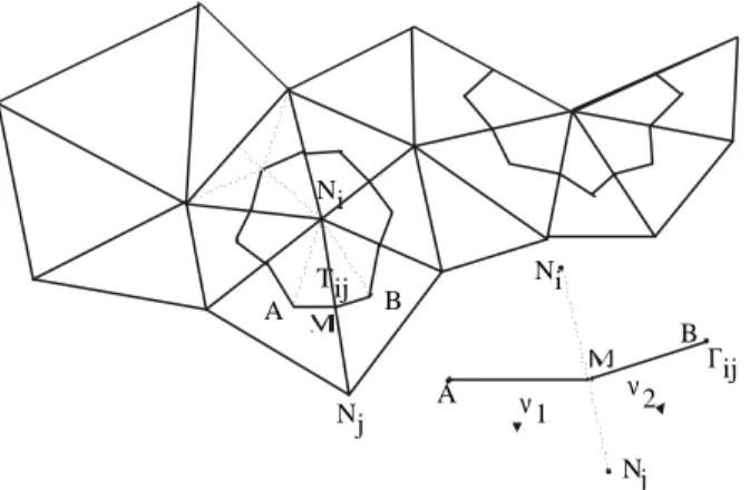
Application of FVM in our case comes from a pre-vious triangle mesh discretization. The vertexes of this triangles are the nodes of the final mesh. For a given node Ni we use the barycentres of the triangles
that have Ni as a common vertex and the middle
point of the triangle side that meets at Ni. The
boundary of the cell of the finite volume Ci is then
obtained by joining these points together as can be seen in Figure 1. This type of FV appears frequently in scientific literature (Godlewsky and Raviart (1996)).
Figure 1. Construction of finite volumes
Working with the SWE in their conservative form and benefit from these equations advantages (Toro, 1997), we carry out a change in notation as follows:
( )
( ) (
G x y w)
y w F x w F t t y x w , , ) , ,
( 1 2 =
∂ ∂ + ∂ ∂ + ∂ ∂ (4)
( )
x,y ∈Ω⊂ R2; t∈[ ]
0,Twhere:
System is written in a more compact form:
( ) (
w G x y w)
t w , , = ⋅ ∇ + ∂ ∂ F (5) where:
( )
(
1( ) ( )
, 2)
; F (F)F w = F w F w T ∇⋅ =div (6)
Now we approximate the exact solution of the equa-tions at the time tn (tn = n∆t) by means of the value Wn, constant in every cell and time step. The first
term is discretized in advance using the Euler method:
t W W
t
w n n
∆ − ≈
∂
∂ +1
(7) Next we integrate the equations over Ci:
( )
(
)
∫∫
∫∫
∫∫
+ ∇⋅ = ∆ − + i i i C n C n C n n dA W y x G dA W dA t y x W y x W , , ) , ( ) , ( 1 F (8)Using the Theorem of Divergence in the second term we change the integral over Ci into an integral
over Γi, boundary of Ci.
Taking into account that Wn, Wn+1 and ∆t are
con-stants, they can be carried out of the integral. Flux and source terms required decentre and upwind schemes. To discretize the flux term we follow the Q-scheme of Van Leer, used in Bermúdez et al
(1998). The discretization of the source term also re-quires an upwind scheme, as it has been recently analysed in Vázquez (1999) and García Navarro et al (2000).
Finally we obtain an explicit in time iterative method allowing us to determinate the variables h,
hu and hv in each node Ni at time tn+1, starting from
the values of these variables at time tn in Ni, and the
nodes Nj surrounding node Ni.
3 MORPHOLOGICAL BLOCK
As previously stated, this part of the code works un-coupled to the hydrodynamic block. The domain in this part, discretized first in triangles and then in
fi- − − = + = + = = ) ( ) ( 0 ; 2 1 2 1 ; 0 0 2 2 2 2 2 1 fy y fx x S S gh S S gh G gh hv huv hv F huv gh hu hu F hv hu h w Tij
A ν2
nite volumes, is exactly the same in order to reduce computational time in solving both processes.
The morphological part of the model uses the previ-ously computed hydrodynamics, so water depth and components of depth-averaged velocity are known. Sediment transport iterations results in evaluation of the bed surface evolution and sediment volumes ex-changed between cells. The existing material must be granular and uniform in all the domain, and an unsteady regime is assured as it will be explained af-terwards in both blocks interactions.
3.1 Continuity equation
The continuity equation for sediment transport by Exner (Exner 1925) allows many kinds of presenta-tion, varying according to the different types of transport. The morphological block calculates the bedload transport with non cohesive sediments, pre-senting here the mentioned continuity equation from García (García, 2000).
(
1)
+(
−)
=0∂ ∂ + ∂ ∂ + ∂ ∂
− s s b
by bx
c E w y q
x q t z
p (9)
where: p = porosity; z = bed surface; (qbx,qby) =
components of bed load transport; ws = fall velocity
of sediment, Es = re-suspension factor, cb = median
concentration of sediment in equilibrium.
First performances using a centred method led to some instabilities, so an upwind scheme was also used in this part of the model. Surface integral de-velopment and divergence theorem application lead to:
(
)
(
(
)
)
− ⋅ −
⋅
− ∆ −
=
∑
Γ+
b s s i
b n
n
c E A
l d q
p t z
z i ν
r r
1
1 (10)
In this case the preceding equation shows an itera-tive explicit method in time, allowing to obtain the bed surface evolution in each node Ni at any interval,
coming from values of the variables in the previous moment, in the node Ni and nodes Nj surrounding it.
3.2 Equations for bed load transport
There are many empirical bed load transport equa-tions in the literature. Morphological block of the model was calibrated with different laboratory ex-periments, using the best relations for the conditions of our studies. In the results included in this paper the analyses have been made with Meyer-Peter&Müller bed load transport formula.
(
)
(
* *)
1.5 350
8
1 c
bs
gd G
q
τ
τ −
=
− (11)
where: τ* = non dimensional shear stress, τ*c = non
dimensional critical shear stress, d50 = mean
diame-ter of sediment, g = gravity, G = specific gravity.
4 COUPLING BLOCKS
The coupling of both parts of the model is as fol-lows. First of all, the hydrodynamic block is run solving the initial hydraulics according to the exist-ing domain and boundary conditions. Reachexist-ing a se-lected convergence, the model enters the morpho-logical block with the computed hydrodynamic data. In this part, the surface evolution (erosion or sedi-mentation) of the nodes is estimated, until one of them exceeds a significant level (3 d50, depending on
d50). When the iteration arrives at this threshold, the
model goes back to the hydrodynamic block, esti-mating new values for hydraulic variables. As con-vergence is reached again, model goes to morpho-logical block and so on. There is a maximum erosion level introduced by the user, although the model may finish execution, if conditions for erosion or deposition disappear in every point of the mesh at any moment.
The model admits any modification in boundary conditions during the process as a part of an un-steady behaviour, re-estimating hydraulic and mor-phological variables with these new data. In case of spilling in downstream border with critical depth, the model may modify this boundary condition turn-ing to the introduced level if erosion leads to that. The real time of the whole process is the correspon-dent to the morphological block, because the time between iterations in the hydrodynamic one is a time of adaptation, that in reality happens at the same time of morphological processes.
5 RESULTS
Some results of the model are presented here. Al-though the model is presented in only one Fortran code, hydrodynamic results are presented previously and separately. Then, an example of the full numeri-cal model is included and compared with the ex-perimental results of the same test. The reason is that the hydrodynamic block was first finished and vali-dated before developing the sediment transport sub-routines.
5.1 Hydrodynamic block
Hydrodynamic part of the model was validated with some particular cases existing in the scientific litera-ture. These examples were not developed with the complete numerical model because of the specific hydraulic problem that they represent, and also be-cause the morphological block is not able to solve some of these particular cases with movable bed. 5.1.1 Channel with an obstacle at the bottom.
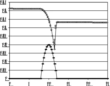
Figure 2 shows the water depth in the axis of sym-metry, in order to be able to compare the results of our 2D model with those obtained in a 1D model and the 1D exact solution.
0 0.05 0.1 0.15 0.2 0.25 0.3 0.35 0.4 0.45
0 5 10 15 20 25
Figure 2. Longitudinal profile (x axis) and depths (y axis) in meters, in a channel with obstacle and with double changing regime.
Due to the presence of the obstacle, it appears a double changing regime, with a clear hydraulic jump in the second one. This result is very similar to the example showed in Vázquez (1999).
5.1.2 Dam-break problem.
It is very frequent in scientific literature to use the dam-break problem for the validation of a model. A domain of 5x200 m without friction at the bottom has been considered, ensuring depths of 1 m and 0.1 m as initial conditions in the two separated areas. Again the water depth in the axis of symmetry, at time t = 25 s, is presented. The ∆t used (0.2 s) is the maximum one in which there are no oscillations, so is equivalent to Courant´s number for one dimen-sion. Results match very well the exact solution as can be seen in Burguete & García-Navarro (2000).
0 0.2 0.4 0.6 0.8 1
0 50 100 150 200
Figure 3. Longitudinal profile (x axis) and depths (y axis) in meters, in a dam-break test in 5x200 m, ∆t=0.2 s, t=25 s.
5.1.3 Settling tanks.
This example, still without experimental validation, represents a double settling tank with dimensions of 4x3 m, a mesh size of 0.05 m, discharge of 0.1 m3/s, downstream depth of 0.25 m and Manning’s coeffi-cient of 0.014. In Figure 4 we can see the stream-lines and eddies properly formed, and fluid separa-tions appearing in different parts of the area in study.
X
0 1 2 3 4
0 0.5 1 1.5 2 2.5 3 3.5
Figure 4. Streamlines in settling tanks of 4x3 m.
5.2 Morphological block.
The complete numerical model (including hydrody-namic and morphological blocks) was run and vali-dated with different experimental tests developed in the Civil Engineering School, University of A Coruña, Spain.
this condition was reached, with sediment transport towards downstream produced by the bed load. In-strumentation tools included a Particle Image Ve-locimetry (PIV) to obtain the whole velocity field and depths in the central section, between points 7.6 and 8.3 (in meters, from upstream). Bed surface ele-vation was obtained from data of PIV and other in-strumentation tools.
The following figures present the results of the com-plete numerical model (hydrodynamic and morpho-logical blocks) and the comparison with the experi-mental data measured in the mentioned test in the axis of symmetry.
Slope was 0.052%, discharge 21.9 l/s, downstream level 0.12 m, mean diameter of sediment of 1 mm and mesh size of 0.1 m.
0 5 10 15 20 25 30 35 40 45 50
7.6 7.7 7.8 7.9 8 8.1 8.2 8.3
Min 10 PIV Min 10 model
Min 40 PIV Min 40 model
Figure 5. Comparison of experimental and numerical results of bed surface elevation (y axis, in mm) versus longitudinal pro-file (x axis, in m) in two time steps
Figure 5 shows a good agreement of the morpho-logical results and the experimental data for bed sur-face evolution. It turns out a better accuracy of the model in higher steps of time until equilibrium is reached in both numerical and experimental tests.
0 5 10 15 20 25 30 35 40 45
0.00 0.10 0.20 0.30 0.40 0.50
min 0 min 10
min 20 min 40
Figure 6. Evolution of bed surface elevation (y axis, in mm) in a cross section located 5.5 meters from upstream the flume (x axis, in m), from beginning to minute 40
Figure 6 also presents a good behaviour of the nu-merical model representing the bed surface evolu-tion of a certain cross secevolu-tion. Similar results were obtained for the rest of the sediment domain in the central part of the flume.
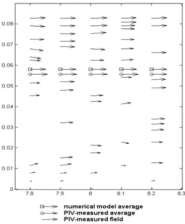
Figure 7. Velocity distribution in longitudinal profile (x axis, in m) versus water depth (y axis, in m). Results of depth-averaged velocity of experimental and numerical tests are also plotted.
6 CONCLUSIONS
The present 2D numerical model developing Finite Volume Method and Shallow Water Equations in unsteady flow represent properly the hydrodynamic
phenomena of many existing problems in scientific literature. Results of the morphological block of the model show the agreement of the bed surface evolu-tion compared with data from laboratory experi-ments, applying laser instrumentation as Particle Im-age Velocimetry. Upwind schemes are used to assure convergence and stability in both parts of the model, and Meyer-Peter&Müller bed load transport formula is found accurate to represent sediment transport evolution.
REFERENCES
Burguete, J. & García-Navarro, P. 2000. An upwind conserva-tive treatment of source terms in shallow water equations.
European Congress on Computational Methods in Applied Sciences and Engineering, Eccomas 2000, Barcelona (Spain)
Bermúdez, A. & Dervieux, A. & Desideri, J.A. & Vá zquez-Cendón, M.E. 1998. Upwind schemes for the two-dimensional shallow water equations with variable depth using unstructured meshes. In Elsevier Science Publishers, Computer Methods in Applied Mechanics and Engineering 155:49-72. Amsterdam (The Netherlands)
Chaudhry, M. 1993. Open channel flow. Prentice-Hall, Inc., New Jersey (USA)
Einstein, H.A. 1950. The bedload function for bedload trans-portation in open channel flows. Technical Bulletin No. 1026, USDA, Soil Conservation Service. USA
Exner, F.M.1925. Über die wechselwirkung zwischen wasser und geschiebe in flüssen. Sitzenberichte der Academie der Wissenschaften, Sec. IIA:134-199. Wien (Austria)
García, M. & Parker G. 1991. Entrainment of bed sediment into suspension. In American Society of Civil Engineer, Journal of Hydraulic Engineering 117:414-435
García, M. 2000. Sedimentation and erosion hydraulics. Hy-draulic Design Handbook, to be published by Mc Graw Hill.
García-Navarro, P. & Vázquez-Cendón, M. E. 2000 On nu-merical treatment of the source terms in the shallow water equations. Computers & Fluids 29 (2000) 951-979.
Godlewsky, E. & Raviart, P. 1996. Numerical approximation of Hyperbolic Systems of Conservation Laws. Springer-Verlag, Berlin
Meyer-Peter, E. & Müller, R. 1948. Formulas for bedload transport. Proceedings of the 2nd Congress of the Interna-tional Association for Hydraulic Research, Stock holm, 39-64
Toro, E.F. 1997. Riemann Solvers and Numerical Methods for fluid Dynamics. A practical introduction. Springer-Verlag, Berlin
Van Rijn, L.C. 1993. Principles of sediment transport in rivers, estuaries and coastal seas. Aqua Publications, Amsterdam (The Netherlands)
Vázquez-Cendón, M.E. 1994. Estudio de esquemas descentra-dos para su aplicación a las leyes de conservación hiper-bólicas con términos fuente. Ph.D. Dissertation, University of Santiago de Compostela, Spain
Vázquez-Cendón, M.E. 1999. Improved treatment of source terms in upwind schemes for the shallow water equations
ins channels with irregular geometry. Journal of Computa-tional Physics 148:497-526