INCOME POLARIZATION IN ARGENTINA:
PURE INCOME POLARIZATION, THEORY AND APPLICATIONS1,2
MATÍAS HORENSTEIN3 AND SERGIO OLIVIERI4
Introduction
The polarization phenomenon is directly linked to the sources of social tension. The notion has its roots in sociology and political science, with Karl Marx arguably being the first social scientist to study it. In economics, its formal analysis has its origins in the nineties, in the work of Esteban and Ray (1991,1994), Foster and Wolfson (1992) and Wolfson (1994). It was subsequently extended, with the ultimate goal of developing not just an index that measured polarization, but also achieving an understanding of the possible causes which may affect it5.
Polarization is a concept that is distinct from inequality, and can be traced to social, economic, and political factors. The motivation for this paper is to analyze the evolution of polarization in Argentina during the unstable period 1998-2002, with the aim of furthering our understanding of the nature of distributive changes.
This work is divided into two main sections: theoretical and empirical. The first has as goal to provide a brief survey of the evolution of the concept of polarization, beginning with an explanation for the simpler case of discrete variables. We subsequently discuss the latest developments in the measurement for the case of continuous variables. We wish to underscore the
1 JEL Classification: D31, D63, I32.
2 We thank Joan Esteban and Jean-Yves Duclos, for their interest and help in the computation of the index.
We also thank Leonardo Gasparini for his teaching and support, Martín Cicowiez for his programming lessons and to the anonymous referee for valuable suggestions which helped us to improve the paper. We also extend our gratitude to Maria Eugenia Garibotti for translating this paper, and to participants and organizers of the November 2004 Network of Inequality and Poverty (NIP) conference held at Universidad de San Andrés, Buenos Aires, Argentina.
3Universidad Nacional de La Plata and CEDLAS (Centro de Estudios Distributivos, Laborales y Sociales),
4Universidad Nacional de La Plata and CEDLAS (Centro de Estudios Distributivos, Laborales y Sociales),
5 Esteban and Ray (1994), Foster and Wolfson (1992), Wolfson (1994), Alesina and Spolaore (1997), Wang
fact that we follow the approach of Esteban and Ray (1994) and Duclos, Esteban and Ray (2004) for discrete and continuous variables respectively6.
The empirical section includes the results for Argentina and their analysis. It starts by tracing the evolution of polarization and comparing it with that of inequality, followed by a look at the robustness of our results and a study of the causes of the change over time – both by considering how the identification effect and the alienation effect affect the index, and by using a micro-simulation technique. It ends with a regional analysis.
I. Polarization: definition and measurement7
A population can be seen as a set of distinct groups that differ in the characteristics of their members. Thus, a group is “similar” to another one when their component members have similar features and “different” when their members have dissimilar characteristics8. A society will be deemed to be polarized when for a given joint distribution of characteristics, the population is clustered around a small number of distant points9. As a society becomes more polarized, conflict will be more likely.
The degree of clustering is important for a large number of social and economic variables. Among the former we find the issues of social class, race, religion, nationality, political parties, etc. In the economic case we find, among others, labor market segmentation and the distribution of firm size within an industry. This notion is also relevant when the defining characteristic of each group is their income.
We would like to emphasize that these first sections are based on the discussion by Esteban and Ray (1994) and Duclos, Esteban and Ray (2004), which should be consulted by the interested reader.
6 For a more detailed treatment of the subject we refer the reader to Esteban and Ray (1994) and Duclos,
Esteban and Ray (2004).
7 The reader who is familiar with the concepts developed in the work of Esteban and Ray (1994) and Duclos,
Esteban and Ray (2004) may skip to the empirical section.
8 Esteban and Ray (1994)
I.1 Polarization and inequality
For a distribution of individual characteristics to be considered polarized, it must display the following characteristics:
1. High level of homogeneity within each group 2. High level of heterogeneity between groups
3. Small number of big groups. In particular, groups of negligible size, such as one individual, should have a small influence on the whole. Each of the previous conditions is linked to the emergence of social tension. In the case of one single person with very different characteristics from the rest, she would not have a significant role in the development of conflict. Thus, if a group consists of individuals who are “similar” among them, we would expect their goals to be the same, or at least similar enough that they feel a strong sense of unity given by their sense of “identification”. In much the same way, the existence of a clear-cut difference between two groups, “alienation” would, ceteris paribus, lead to an increase in social tension. In other words, the goals of each group may conflict.
Esteban and Ray thus define a framework within which polarization may be summarized as the interaction between the identification and alienation that each individual feels with respect to the rest (IA).
The three postulates that were mentioned above allow us to clarify the difference between this concept and inequality. In order to capture the first feature, assume the existence of two distributions of income across a population, in two moments of time. In the first moment, population is evenly spread among 10 income values separated by a gap of one unit each. At time 2 the population is uniformly distributed between two income groups, clustered around points three and eight.
In the following figures we can observe that the second distribution is more polarized than the first. There exist two perfectly defined groups, which generate a high degree of identification when compared to the first, where the sense of group is vague. In the second distribution people are either “rich” or “poor”, without the presence of a “middle class” to bridge the gap. This can be regarded as a situation with higher tension than that in the initial period.
Figure 1
1 2 3 4 5 6 7 8 9 10 1 2 3 4 5 6 7 8 9 10
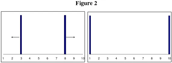
It could further happen that income is concentrated in two peaks, but instead of 3 and 8 they are 1 and 10. Going to this case from the first distribution leads to higher heterogeneity between groups, or “alienation”, as well as resulting in increased homogeneity within each group. In contrast to our previous argument, it is not just polarization that would grow, but inequality as well. Thus, we cannot assert that polarization and inequality are always at odds with each other.
Figure 2
1 2 3 4 5 6 7 8 9 10 1 2 3 4 5 6 7 8 9 10
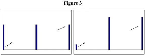
In order to interpret the third characteristic, we will consider a population that is distributed across three equally spaced points. Initially, the mass in the center and right are approximately the same. At a second stage, there is a small shift from the left end to the right. The problem is now more complex than in the first two cases. Despite the fact that such a move would tend to create two distinctly defined groups, the mass in the left could have originally been an instrument to introduce social tension, and the net effect is therefore not clearly defined.
[image:4.595.154.440.400.505.2]Figure 3
Two examples of polarization measures for discrete variables are the Wolfson and the Esteban, Gardin and Ray (1999) indices:
Wolfson:
⎥⎦ ⎤ ⎢⎣
⎡ − −
=
2 ) 5 . 0 ( 5 .
0 L G
m
PW µ
where µ= mean, m= median, L(0.5) = value of the Lorenz curve at the median income and G = Gini coefficient.
Esteban, Gardin and Ray (1999):
[
( ) ( *)]
*) , ( ) , ; ,
(F nα β P α ρ β G f G ρ
PEGR ≡ ER − −
where:
∑∑
−= +
i j
j i j i ER
*) , (
P α ρ π1απ µ µ , α =identification factor, vector
of values that include bounds, quantity of individuals, and the mean income for each group that minimizes inequality within each of the n groups.
=
*
ρ
G(f) = Gini coefficient for the whole population
G(
ρ
*)= Gini coefficient for the population defined byρ
*assuming that individuals are pre-assigned to n groups, and proposes a methodology to define the location of each group10.
I. 2 The income polarization index
In the previous subsection we identified two forces that affect each individual: identification and alienation. Given that polarization is related to social tension, the measure that summarizes it must take into account both factors. Should any of those be absent, any antagonism would be eliminated.
Two problems arise when applying polarization indexes defined in terms of discrete variables to continuous variables, such as income, consumption, and the like. On the one hand, continuous changes in polarization are not captured in some cases, given that the population is divided into a finite number of groups. The ER (1994)11 indexes have this problem.
On the other hand, these indices assume that the population is already divided into a small number of relevant groups12. In other words, there is a certain degree of arbitrariness in the choice of number of groups. For instance, the Wolfson index implicitly assumes the population is divided into two groups of similar size, and this precludes the accurate detection of changes in polarization when there exist more than two mass points. Another instance is provided by EGR (1999), who leave the definition of the number of groups or poles into which to divide the population to the researcher’s discretion.
The Duclos-Esteban-Ray index (DER)13, sets out to solve these problems. In order to do so, they redefine the axioms that must be satisfied by a polarization index for continuous variables and present a measure of “pure income polarization”. This new index allows for individuals not to be clustered around discrete income intervals, and lets the size of each group be determined by nonparametric kernel techniques, avoiding arbitrary choices.
The following axioms that are satisfied by the DER index are based on a density with finite support (kernel), and symmetric reductions in dispersion that concentrate the density around its mean (squeezes).
10
For a more thorough analysis of each of the measures we refer the reader to: Wolfson (1994), Esteban, Gardin and Ray (1999)
11
Esteban and Ray (1994) pp 845-847
12 Esteban and Ray (1994)
Axiom 1: if a distribution is made up of a basic density, then a squeeze cannot increase polarization.
In
Axiom 2: if a symmetric distribution is composed by three basic densities then a squeeze in the outer densities should not reduce polarization.
Axiom 3: if we consider a symmetric distribution made up of four basic densities with disjoint supports, then a move of the center distributions towards their outer neighbors, while keeping the disjoint supports, should increase polarization.
come
Income
Axiom 4: Given two distributions F and G, if P(F) ≥ P(G), being P(F) and
P(G) the respective polarization indexes, it must be that P(
α
F) ≥ P(α
G),where
α
F andα
G represent a rescaled version of F and G.In this manner, the authors establish that a general polarization measure that respects the previous axioms must be proportional to:
∫∫
− ≡ + dydx x y ) y ( f ) x ( f ) f (Pα 1α
Remark that in order to respect the axioms the
α
parameter must lie within the interval [0.25, 1]14. The formula can be rewritten as:∫
= f(y) g(y)dF(y) )
F (
Pα α
Where g(y) captures the “alienation” effect, and f(y)
α
the “identification”. It is interesting to note that withα
=0, the polarization index coincides with the Gini coefficient15.If we have a sample of incomes with independent and identically distributed observations ranked from smallest to highest, the indicator’s operational formula is:
⎥ ⎥ ⎦ ⎤ ⎢ ⎢ ⎣ ⎡ ⎟ ⎟ ⎠ ⎞ ⎜ ⎜ ⎝ ⎛ ⎟ ⎟ ⎠ ⎞ ⎜ ⎜ ⎝ ⎛ − − ⎟ ⎟ ⎠ ⎞ ⎜ ⎜ ⎝ ⎛ − ⎟ ⎟ ⎠ ⎞ ⎜ ⎜ ⎝ ⎛ − + =
∑
∑
∑
− = − = − = − 1 1 1 1 1 11 2 1 2i
j i i j j i j i j i n i
i) ˆ y w w w w w y w y
y ( fˆ n ) Fˆ (
Pα α µ
Where yi is the ith individual income, µˆ is the sample mean, wi is the weight
of individual i, and
∑
= = n j j w w 1 .
14
The infimum and supremum of the interval follow from axioms 2 and 1 respectively.
15 For a more detailed analysis of how the parameter affects the indicator, read Duclos, Esteban and Ray
The function is a nonparametric kernel estimate of the income density, using a bandwidth that minimizes the mean square error of the estimator h
) y ( fˆ i *, given by: ) n ( o n ) dy ) y ( P ) y ( f ( )) y ( P ), y ( a cov( * h k '' 1 2 2 2 1 − − + =
∫
α α α ασ with∫
+ ∞∫
− + + = y ) x ( dF ) x ( f ) y x ( ) x ( dF ) x ( f y ) y ( P ) ( ) y (aα 1 α α α 2 α
Duclos, Esteban and Ray (2004) provide other formulas that are easier to compute. The first can be used with normal distributions and will not exceed the h* that minimizes the means square error by more than 5%.
1 5 7
4 − −
≅ . n σα
* h
The second is for distributions with skewness greater than 6:
) ( ln ln ) * . ( ) . . ( IQ n * h α σ σ 15323 7268 4 5 10 09 1 1 7 14 76 3 + − − + + ≅
where IQ is the interquantile range, and
σ
in is the variance of log-income.II.Application
II.1 Methodological aspects
The polarization indices are computed using the October wave of the Encuesta Permanente de Hogares (Permanent Household Survey – EPH) for the years 1998 to 2002. These include 28 urban conglomerates that allow the country to be divided into six regions: Greater Buenos Aires (GBA), Región Pampeana, Cuyo, Noroeste (NOA), Noreste (NEA) and Patagonia16.
The variable we study is the mean normalized income per equivalent adult using the official equivalent adult scale of the Instituto de Estadísticas and Censos (INDEC). The observations with negative income and those that were more than 20 times the median were eliminated, as were those that the Institute discards17.
II.2Results
II. 2.1 Evolution and Causes
Evolution
The following table presents the evolution of the income polarization index in Argentina during the period 1998 to 200218, evaluated at different weights for the identification factor.
16 GBA: City of Buenos Aires and Greater Buenos Aires; PAMPEANA: La Plata, Bahía Blanca, Rosario,
Santa Fe, Paraná, Córdoba, Concordia, Santa Rosa, Mar del Plata and Río Cuarto; CUYO: Mendoza, San Juan and San Luis; NOA: Catamarca, Salta, La Rioja, Tucumán, Santiago del Estero and Jujuy; NEA: Corrientes, Formosa, Resistencia and Posadas; and PATAGONIA: Comodoro, Rivadavia, Neuquén, Río Gallegos, Tierra del Fuego and Alto Valle del Río Negro.
17 Zero income observations are eliminated because we observe substantial variation in the proportion of
individuals with zero income in different years. These changes presumably come from better recording of low income individuals.
18
Table 1: Polarization and Inequality – Countrywide
Polarization
OBS
Source: Authors’ elaboration based on EPH-INDEC data.
We observe that the index increased throughout the period, regardless of the choice of alpha. Furthermore, the evolution was similar to that of the inequality index – recall that if
α
=0 the polarization index equals the Gini coefficient.The validity of the increase in polarization can be tested by using bootstrapping or resampling methods. This technique allows us to build 95% confidence intervals, thereby enabling us to test for the existence of a significant change. We find there is a significant change whenever these intervals do not overlap.
We performed the analysis on the polarization indexes with parameters 0.5 and 0.75, given that values nearby 0.25 and 1 may conflict with some of the axioms19.
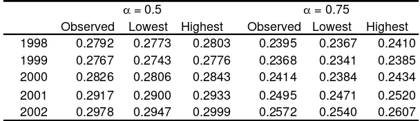
Table 2: Confidence intervals for polarization indexes (100 bootstrap samples)
Source: Authors’ elaboration based on EPH-INDEC data.
19 Duclos, Esteban and Ray (2004) pp. 1744 and 1758.
0 0.25 0.5
α
0.75 1
1998 0.4851 0.3477 0.2792 .23950 0 .2135 92754 1999 0.4817 0.3450 0.2767 .23680 0 .2104 85343 2000 0.4940 0.3532 0.2826 .24140 0 .2144 77343 2001 0.5139 0.3650 0.2917 .24950 0 .2220 76945 2002 0.5181 0.3701 0.2978 .25720 0 .2315 77001
Observed Lowest Highest Observed Lowest Highest 1998 0.2792 0.2773 0.2803 0.2395 0.2367 0.2410 1999 0.2767 0.2743 0.2776 0.2368 0.2341 0.2385 2000 0.2826 0.2806 0.2843 0.2414 0.2384 0.2434 2001 0.2917 0.2900 0.2933 0.2495 0.2471 0.2520 2002 0.2978 0.2947 0.2999 0.2572 0.2540 0.2607
[image:11.595.145.449.527.615.2]From table 2 we can tell that for
α
= 0.5 the yearly increases are significant from 1999 to 2002. Furthermore, forα
= 0.75 these increases were significant from 2000 onward. Thus, when comparing the endpoints of theperiod under s n t tne c y, but
also turned ou o n ri n
199820. so si r ng sta od.
As s t e ica ity la may
show o b . re s d in
[image:12.595.167.426.306.416.2]different prop t o po e t
Figure 3: tudy, Arge
t
tina no only wi la
ssed an in o
rease in b
inequalit 2
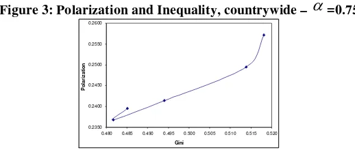
t o have a more p rized i c me dist ution i 002 than in In other words, “ cial ten on” inc eased duri this un ble peri was ta ed in th theoret l section, inequal and po rization pposite ehavior In figu 1 we how how the indexes change
or ions, alm st in op site dir c ions.
Polarization and Inequality, countrywide –
α
=0.750.2400 0.2450 0.2500 0.2550 0.2600
Po
la
r
iza
ti
o
n
0.2350
0.480 0.485 0.490 0.495 0.500 0.505 0.510 0.515 0.520
Gini
Source: Authors’ elaboration based on EPH-INDEC data.
If w s arization
we find t n the pure
polarization index. However, these results should be interpreted cautiously, bearing in mind the limitations described above.
Table 3: Bipolarization – Argentina Income per Equivalent Adult
e compare the new index with the discrete measure of pol hat the results for Argentina had the same upward tre d than
EGR Wolfson
α = 0.5 α = 0.75
1998 0.279 0.239 0.154 0.441
2000 0.283 0.241 0.158 0.459
DER
2002 0.298 0.257 0.167 0.483
Source: Gasparini, L., “Argentina’s distributional failure” (IADB, September 18, 2003)
[image:12.595.191.404.528.586.2]
Possible causes for po
To further interpret the change in polarization it is helpful to show how each income level adds to the total value of the index. The following figures display three curves: income density (de), the polarization curve (po) and the alienation curve (gi). The integral of the polarization curve is the value of the polarization index, while the integral of the alienation curve is the Gini
coefficient. In grals is the
[image:13.595.146.451.353.465.2]entification the integral of the density function quals 1.
Figure 4: Polarization, Inequality and Density – Countrywide
larization
addition, the difference between these two inte factor. By construction,
id e
(Income per equivalent adult 1998-2002)
Polarization (alfa=0.75) and Inequality - arg_98
0
.2
5
.5
.7
5
1
gi
/p
o
/d
e
0 .5 1 1.5 2 2.5
Mean Normalized Income per Equiv alent Adult
gi po de
0
Polarization (alfa=0.75) and Inequality - arg_02
.2
5
.5
.7
5
1
gi
/p
o
/d
e
0 .5 1 1.5 2 2.5
Mean Normalized Income per Equiv alent Adult
gi po de
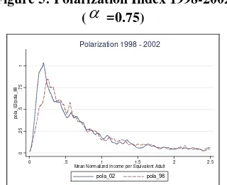
Figure 5: Polarization Index 1998-2002
Source: Authors’ elaboration based on EPH-INDEC data.
(
α
=0.75)0
.2
5
.5
.7
5
1
po
la
_0
2/
p
ol
a_9
8
0 .5 1 1.5 2 2.5
Mean Normalized Income per Equiv alent Adult
pola_02 pola_98
Polarization 1998 - 2002
[image:13.595.218.378.495.625.2]From the previous figures we can observe that all curves become more
leptokurtic and asym dividuals provide a
larger share of both polarization nd lity. This increase can be seen clearly by superimposing the polarization curves for 1998 and 2002 (Figure 5). The increase in polarization at the lowest income levels was thus brought about by more intense alienation of the groups with highest identification. Ceteris paribus, there will be higher polarization the higher the correlation between identification and alienation.
This change in polarization reflects an increase in potential conflict, or tension, especially among income groups with 0 to 0.5 of the normalized income per equivalent adult. These added 0.12 and 0.15 index points in 1998 and 2002, respectively. This represents an increase in overall participation from
22
metric. This means that low-income in a inequa
54% to 59%
To further inquire as to the source of these changes we performed a micro-decomposition of the labor income per equivalent adult. This technique is based upon the computation of different distributions, the actual distribution for year t, and that resulting from simulating the labor income of each
of total polarization in each year21.
individual in year t by fixing some argument of their income-determination function at the level of another year, t’. The arguments considered include observable and unobservable characteristics of the individuals, and the parameters that link observable characteristics with wages .
The decomposition of the change in the DER polarization index was performed for the years 1998 and 2002 for values of the alpha parameter 0.5 and 0.75, changing education levels of the population, and parametric estimates of returns to education, gender gap, returns to experience, region effects, and unobservable factors. The methodology was based on Gasparini, Marchionni, and Sosa Escudero (2005)23.
Given that the micro-simulation technique is path-dependent, we alternatively used 1998 and 2002 as base years and computed the average changes. Since these are not sensitive to the choice of alpha, we will conduct the analysis considering alpha = 0.75.
21
To trace the evolution throughout the period, refer to the appendix.
g computation of micro-simulations.
22 Gasparini, L, Marchionni, M and Sosa Escudero, W (2001)
T
16 0.01 21.51 0.01 Returns to Experience 26.23 0.07 21.57 0.07
Region 26.26 0.10 21.65 0.15
Unobservables 28.09 1.93 23.37 1.87
Coefficients 1998
Indicator Change Level Change
1998 Observed 26.16 2.15 21.50 2.12 2002 Observed 28.31 23.62
Effects
Characteristics 28.19 0.12 23.48 0.14 Returns to Education 28.16 0.15 23.49 0.13 Gender Gap 28.29 0.01 23.61 0.01 Returns to Experience 28.13 0.18 23.45 0.17
Region 28.10 0.21 23.36 0.25
Unobservables 26.82 1.49 22.22 1.40
able 3: Decomposition of the change in the polarization index of equivalent labor income
Coefficients 2002
Indicator Change Change
1998 Observed 26.16 21.50 α = 0.5 α = 0.75
2002 Observed 28.31 2.15 23.62 2.12 Effects
Characteristics 26.13 -0.03 21.46 -0.04 Returns to education 26.21 0.06 21.56 0.06
Gender Gap 26.
α = 0.5
Source: Authors’ elaboration based on EPH-INDEC data.
Average Change
α=0.5 α=0.75 Indicator Change Change
1998-2002 Observed 2.15 2.12 Effects
Characteristics 0.05 0.05 Returns to Education 0.10 0.10
Gender Gap 0.01 0.01
Returns to Experience 0.13 0.12
Region 0.15 0.20
Unobservables 1.71 1.64
α = 0.75
Level Level
Results show that on average all the effects led to an increase i 002
n polarization between 1998 and 2 rvable factors account for 77% of the dex, followed by region (9%), returns to experience (6%) and to education (5%). The lowest explanato er comes from individu teristics %) and r .
II.2.2 Region n and a arison to inequality
In t n we ver hat ng
the labor t captured by regional factors wa ost rtant. This
motivate indicat sis in this section is
intended as an illustration, e an is tistic gnificance remains
When analyzing polarization within regions in the period 1998 to 2002, we observe an upward trend, just as in the country as a whole, in all regions except NEA. we compare this w regiona y index, the rankings ithin the ame ye p on a pha under consideration. For instance, in 1998 anki de from uality and polarization (with an alpha of 0.5) are i entical, while there are differences if alpha is onsidering the ges ank or bo
becomes and pola region of t untry enation in this regi t intense where i icati as est.
Another interesting case is NOA, which witnessed an increase in alienation, while the identificatio ect pe this ct almost complete an almost con pola ion x wh
0.75.
24. Unobse change in the in
ry pow (0.4%)25
al charac (2 gende
al polarizatio comp
he previous sectio ified t amo the observable effects in
market tha s the m impo
s the analysis of the or by region. The analy
mainly as th alys of sta al si
to be done.
If differ w
ith the l inequalit s ar, de ending the v lue of al
ineq the r ngs rived
d
0.75. When c chan in r ing f th years, GBA the most unequal rized he co . Ali
on was mos dentif on w high
n eff dam ned impa
ly, achieving stant rizat inde en alpha equals
24 Only the educational characteristics effect had a versa een both years, with the average effect
being positive. For reasons such as this, the average d be i eted cautiously.
25 We cannot over inants of polarization in Argentina.
In particul ues of macroeconomic instability.
sign re l betw
shoul nterpr
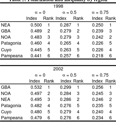
Table 5: Polarization and Inequality by region
Index Rank Index Rank Index Rank
NEA 0.500 1 0.287 1
Source: Authors’ elaboration based on EPH-INDEC data.
Index Rank IndexRank Index Rank
GBA 0.532 1 0.299 1 0.256 1
NOA 0.497 2 0.284 3 0.245 3
NEA 0.495 3 0.286 2 0.246 2
Patagonia 0.482 4 0.276 5 0.235 5
Cuyo 0.480 5 0.279 4 0.240 4
Pampeana 0.479 6 0.276 6 0.234 6
As is evident, inequality and polarization rankings differ. Two regions that provide an example of this are NEA and Patagonia. A comparison of all three curves in both regions for the year 2002 allows us to note that the structure of inequality and polarization are quite different. The distribution in the Northeast displays greater polarization at income levels below one half of the mean, when we compare it with Patagonia. In NEA, this income level represents 0.14 index points, which amounts to roughly 58% of the total. Patagonia, on the other hand, has a lower polarization for this same income level (11% lower).
0.250 1
GBA 0.489 2 0.279 2 0.239 3
Patagonia 0.460 4 0.265 4 0.226 5
NOA 0.483 3 0.279 3 0.242 2
Cuyo 0.445 5 0.263 5 0.226 4
Pampeana 0.441 6 0.257 6 0.218 6
2002
α = 0 α = 0.5 α = 0.75
Figure 6: Polarization and Inequality in Patagonia (R5) and NEA (R – 2002 (6)
α
= 0.75)0 .2 5 .5 .7 5 1 gi /p o /d e
0 .5 1 1.5 2 2.5
Mean Normalized Income per Equiv alent Adult
gi po de
Polarization (alfa=0.75) and Inequality - arg_02 - R_5 Polari
0 .2 5 .5 .7 5 1 gi /p o /d e
1 1.5 2 2.5
Mean Normalized Income per Equiv alent Adult
gi po de
fa=0. - R_6 zation (al 75) and Inequality - arg_02
0 .5
Note: gi: alienation curve; po: tion curve tification
Source: Authors’ elab EP .
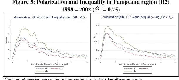
A final ple is by eana region, which had the highest increase in polarization index with an alpha o . I he following gr 99 2 2, n bser w goes from a
relatively fla c o struc a s concentrated
in the low-in a cl rly d quit
for the country as a whole2 o people with incomes below ha
polariza b
; de: iden curve
oration ased on H-INDEC data
exam provided the Pamp
f 0.75 f we look at t aphs for 1
imodal polarization
8 and 00 we ca o ve ho it t, mult urve t a ture th t i
come levels nd is
6. The share in t ea unimo
he polarization index
al, e similar to what is true f
lf the mean went from 44% to 53%.
Figure 5: Polarization and Inequality in Pampeana region (R2) 1998 – 2002 (
α
= 0.75)0 .2 5 .5 .7 5 1 gi /p o /d e
0 .5 1 1.5 2 2.5
lized Income per Equiv alent Adult Mean Norma
gi po de
Polarization (alfa=0.75) and Inequality - arg_98 - R_2
0
Polarization (alfa=0.75) and Inequality - arg_02 - R_2
.2 5 .5 .7 5 1 gi /po /de
0 .5 1 1.5 2 2.5
Mean Normalized Income per Equiv alent Adult
gi po de
Note: gi: alienation curve; po: polarization curve; de: identification curve Source: Authors’ elaboration based on EPH-INDEC data.
26 To follow the evolution of inequality and polarization throughout the period in different regions, refer to
[image:18.595.143.448.472.609.2]Conclusions
The analysis of income polarization in Argentina, following the new methodology proposed by Duclos-Esteban-Ray for continuous variables, revealed a significant increase between 1998 and 2002, for various values of the identification parameter.
This increase in “social tension” was fueled by two effects: the first was an increase in homogeneity within the group of low-income individuals; the second was an increase in heterogeneity between this group and the rest.
We explored different causes by means of a micro-decomposition technique, finding that on average all effects we considered increased
polari change came from
e distrib nts were found to be of
od
On n
increase ith an
associated increase of the correlation between identification and alienation. This change had different intensity throughout the regions, leading to distinct levels of “tension” within the country.
zation between 1998 and 2002. Although most of the th
m
ution of unobservable factors, three eleme
erate importance: region, returns to education and returns to experience. The gender gap did not have any effects, while educational achievement reinforced the increase on average, but the sign of this effect was found to depend on the choice of the base year.
An exploratory analysis by region showed that the rankings according to polarization and inequality might differ, depending on the choice of alpha. We also found that polarization increased across regions, with the exception of
EA. N
References
lesina, A. and Spolaore, E. (1997), “On the Number and Size of Nations”
Qua
Duc
1999), “Extensions of the measure of Pola
etrica 62, (4), November, pp. 819-852.
hanges Through Microeconometric Decompositions: The Case of Greater Buenos Aires” in Bourguignon, F, Ferreira, F and Lustig, N, The microeconomics of income distribution
dynamics (In East Asia and Latin America), Oxford University Press, pp.
47-83
Gasparini, L., Marchionni, M. and Sosa Escudero, W. (2001), “Distribución del Ingreso en la Argentina: Perspectivas y Efectos sobre el Bienestar”, Premio Fulvio Salvador Pagani.
A
rterly Journal of Economics, 113, pp. 1027-1056.
Busso, M. (2003), “A Note on Income Polarization”, Universidad Nacional de La Plata Argentina.
D’ Ambrosio, C. and Wolf, E. (2001), “Is Wealth Becoming More Polarized in The United States?” Working paper 330, Levy Economics Institute, Bard College.
los, J., Esteban, J. and Ray, D. (2003), “Polarization: Concepts, Measurements, Estimation”, CIPRÉE, Canada.
Duclos, J., Esteban, J. and Ray, D. (2004), “Polarization: Concepts, Measurements, Estimation”, Econometrica 72 (6), November, pp. 1737-1772.
Esteban, J. (2002), “The Measurement of Polarization: a Survey and an Application”, CSIC, November.
Esteban, J., Gardín, C. and Ray, D. (
rization, with an application to the income distribution of five OECD countries”, mimeo, Instituto de Análisis Económico.
Esteban, J. and Ray, D. (1994), “On the Measurement of Polarization”
Econom
Foster, J. and Wolfson, M. (1992), “Polarization and the Decline of the Middle Class: Canada and the US”, mimeo, Vanderbilt University.
Gasparini, L. (2003), “Argentina’s Distributional Failure: The Role of tegration and Public Policies” Interamerican Development Bank, Brasilia,
in Latin America” in
and Tsui, K. (2000) “Polarization Orderings and New Classes of
erges”, American Economic
In
September.
Gasparini, L. (2004), “Different Lives: Inequality
Ferranti, Perri, et al. Inequality In Latin America: Breaking with History?
World Bank.
Schimdt, A. (2000), “Statistical Measurement of Income Polarization. A Cross-National Comparison” University of Cologne, Germany.
Wang, A.
Polarization Indices” Journal of Public Economic Theory, 2, pp. 349-363.
Wolfson, M. (1994), “When Inequality Div
Review, 84, pp 353-358.
Graphical Appendix
ARGENTINA
0
.2
5
.5
.7
5
1
gi
/po
/de
0 .5 1 1.5 2 2.5
Mean Normalized Income per Equiv alent Adult
gi po de
Polarization (alfa=0.75) and Inequality - arg_98 Polarization (alfa=0.75) and Inequality - arg_99
1
0
.2
5
.5
.7
5
gi
/p
o
/de
0 .5 1 1.5 2 2.5
Mean Normalized Income per Equiv alent Adult
gi po de
0
.2
5
.5
Polarization (alfa=0.75) and Inequality - arg_00
.7
5
1
gi
/p
o
/de
0 .5 1 1.5 2 2.5
Mean Normalized Income per Equiv alent Adult
gi po de
0
.2
5
.5
Polarization (alfa=0.75) and Inequality - arg_01
.7
5
1
gi
/po
/de
0 .5 1 1.5 2 2.5
Mean Normalized Income per Equiv alent Adult
gi po de
0
.2
5
.5
.7
5
1
gi
/p
o
/de
0 .5 1 1.5 2 2.5
Mean Normalized Income per Equiv alent Adult
gi po de
Greater Buenos Aires (R_1) Región Pampeana (R_2) 0 .2 5 .5 .7 5 1 gi /po /de
0 .5 1 1.5 2 2.5
Mean Normalized Income per Equiv alent Adult gi po de
Polarization (alfa=0.75) and Inequality - arg_98 - R_1
0 .2 5 .5 .7 5 1 gi /po /d e
0 .5 1 1.5 2 2.5
Mean Normalized Income per Equiv alent Adult gi po de
Polarization (alfa=0.75) and Inequality - arg_98 - R_2
0 .2 5 .5 .7 5 1 gi /po /de
0 .5 1 1.5 2 2.5
Mean Normalized Income per Equiv alent Adult gi po de
Polarization (alfa=0.75) and Inequality - arg_99 - R_1
0 .2 5 .5 .7 5 1 gi /po /de
0 .5 1 1.5 2 2.5
Mean Normalized Income per Equiv alent Adult gi po de
Polarization (alfa=0.75) and Inequality - arg_99 - R_2
0 .2 5 .5 .7 5 1 g i/ po/ de
0 .5 1 1.5 2 2.5
Mean Normalized Income per Equiv alent Adult gi po de
Polarization (alfa=0.75) and Inequality - arg_00 - R_1
0 .2 5 .5 .7 5 1 g i/ po/ de
0 .5 1 1.5 2 2.5
Mean Normalized Income per Equiv alent Adult gi po de
Polarization (alfa=0.75) and Inequality - arg_00 - R_2
0 .2 5 .5 .7 5 1 gi /p o /d e
0 .5 1 1.5 2 2.5
Mean Normalized Income per Equiv alent Adult gi po de
Polarization (alfa=0.75) and Inequality - arg_01 - R_1
0 .2 5 .5 .7 5 1 gi /p o /d e
0 .5 1 1.5 2 2.5
Mean Normalized Income per Equiv alent Adult gi po de
Polarization (alfa=0.75) and Inequality - arg_01 - R_2
0 .2 5 .5 .7 5 1 gi /p o /d e
0 .5 1 1.5 2 2.5
Mean Normalized Income per Equiv alent Adult gi po de
Polarization (alfa=0.75) and Inequality - arg_02 - R_1
0 .2 5 .5 .7 5 1 gi /p o /d e
0 .5 1 1.5 2 2.5
Mean Normalized Income per Equiv alent Adult gi po de
Cuyo (R_3) NOA (R_4) 0 .2 5 .5 .7 5 1 gi /po /de
0 .5 1 1.5 2 2.5
Mean Normalized Income per Equiv alent Adult gi po de
Polarization (alfa=0.75) and Inequality - arg_98 - R_3
0 .2 5 .5 .7 5 1 gi /po /de
0 .5 1 1.5 2 2.5
Mean Normalized Income per Equiv alent Adult gi po de
Polarization (alfa=0.75) and Inequality - arg_98 - R_4
0 .2 5 .5 .7 5 1 gi /po /de
0 .5 1 1.5 2 2.5
Mean Normalized Income per Equiv alent Adult gi po de
Polarization (alfa=0.75) and Inequality - arg_99 - R_3
0 .2 5 .5 .7 5 1 gi /po /de
0 .5 1 1.5 2 2.5
Mean Normalized Income per Equiv alent Adult gi po de
Polarization (alfa=0.75) and Inequality - arg_99 - R_4
0 .2 5 .5 .7 5 1 gi /po/ d e
0 .5 1 1.5 2 2.5
Mean Normalized Income per Equiv alent Adult gi po de
Polarization (alfa=0.75) and Inequality - arg_00 - R_3
0 .2 5 .5 .7 5 1 gi /po/ d e
0 .5 1 1.5 2 2.5
Mean Normalized Income per Equiv alent Adult gi po de
Polarization (alfa=0.75) and Inequality - arg_00 - R_4
0 .2 5 .5 .7 5 1 gi /po/ d e
0 .5 1 1.5 2 2.5
Mean Normalized Income per Equiv alent Adult gi po de
Polarization (alfa=0.75) and Inequality - arg_01 - R_3
0 .2 5 .5 .7 5 1 gi /po/ d e
0 .5 1 1.5 2 2.5
Mean Normalized Income per Equiv alent Adult gi po de
Polarization (alfa=0.75) and Inequality - arg_01 - R_4
0 .2 5 .5 .7 5 1 gi /po /d e
0 .5 1 1.5 2 2.5
Mean Normalized Income per Equiv alent Adult gi po de
Polarization (alfa=0.75) and Inequality - arg_02 - R_3
0 .2 5 .5 .7 5 1 gi /po /d e
0 .5 1 1.5 2 2.5
Mean Normalized Income per Equiv alent Adult gi po de
Patagonia (R_5) NEA (R_6) 0 .2 5 .5 .7 5 1 gi /po /de
0 .5 1 1.5 2 2.5
Mean Normalized Income per Equiv alent Adult gi po de
Polarization (alfa=0.75) and Inequality - arg_98 - R_5
0 .2 5 .5 .7 5 1 gi /po /d e
0 .5 1 1.5 2 2.5
Mean Normalized Income per Equiv alent Adult gi po de
Polarization (alfa=0.75) and Inequality - arg_98 - R_6
0 .2 5 .5 .7 5 1 gi /po /d e
0 .5 1 1.5 2 2.5
Mean Normalized Income per Equiv alent Adult gi po de
Polarization (alfa=0.75) and Inequality - arg_99 - R_5
0 .2 5 .5 .7 5 1 gi /po /d e
0 .5 1 1.5 2 2.5
Mean Normalized Income per Equiv alent Adult gi po de
Polarization (alfa=0.75) and Inequality - arg_99 - R_6
0 .2 5 .5 .7 5 1 gi /po /d e
0 .5 1 1.5 2 2.5
Mean Normalized Income per Equiv alent Adult gi po de
Polarization (alfa=0.75) and Inequality - arg_00 - R_5
0 .2 5 .5 .7 5 1 gi /po /d e
0 .5 1 1.5 2 2.5
Mean Normalized Income per Equiv alent Adult gi po de
Polarization (alfa=0.75) and Inequality - arg_00 - R_6
0 .2 5 .5 .7 5 1 gi /po /d e
0 .5 1 1.5 2 2.5
Mean Normalized Income per Equiv alent Adult gi po de
Polarization (alfa=0.75) and Inequality - arg_01 - R_5
0 .2 5 .5 .7 5 1 gi /po /d e
0 .5 1 1.5 2 2.5
Mean Normalized Income per Equiv alent Adult gi po de
Polarization (alfa=0.75) and Inequality - arg_01 - R_6
0 .2 5 .5 .7 5 1 gi /p o /d e
0 .5 1 1.5 2 2.5
Mean Normalized Income per Equiv alent Adult gi po de
Polarization (alfa=0.75) and Inequality - arg_02 - R_5
0 .2 5 .5 .7 5 1 gi /p o /d e
0 .5 1 1.5 2 2.5
Mean Normalized Income per Equiv alent Adult gi po de
Table Appendix
Regional Polarization
0.4950
1998 0.25 0.3477 0.3491 0.3204 0.3243 0.3452 0.3315 0.3549 1999 0.25 0.3450 0.3458 0.3221 0.3305 0.3360 0.3346 0.3541 2000 0.25 0.3532 0.3542 0.3296 0.3434 0.3413 0.3310 0.3559 2001 0.25 0.3650 0.3692 0.3402 0.3427 0.3500 0.3249 0.3672 2002 0.25 0.3701 0.3751 0.3449 0.3463 0.3532 0.3460 0.3547
1998 0.50 0.2792 0.2794 0.2571 0.2625 0.2791 0.2655 0.2869 1999 0.50 0.2767 0.2767 0.2577 0.2667 0.2700 0.26 0.2839 2000 0.50 0.2826 0.2829 0.2628 0.2755 0.2734 0.2641 0.2849 2001 0.50 0.2917 0.2941 0.2710 0.2723 0.2796 0.2590 0.2937 2002 0.50 0.2978 0.2990 0.2757 0.2791 0.2839 0.2764 0.2857
1998 0.75 0.2395 0.2387 0.2181 0.2259 0.2423 0.2259 0.2496 1999 0.75 0.2368 0.2365 0.2178 0.2286 0.2313 0.2259 0.2438 2000 0.75 0.2414 0.2414 0.2210 0.2357 0.2338 0.2232 0.2446 2001 0.75 0.2495 0.2512 0.2282 0.2297 0.2384 0.21 0.2516 2002 0.75 0.2572 0.2557 0.2338 0.2402 0.2449 0.234 0.2462
1998 1 0.2135 0.2117 0.1910 0.2015 0.2190 0.1992 0.2262 1999 1 0.2104 0.2099 0.1902 0.2033 0.2058 0.1981 0.2178 2000 1 0.2144 0.2141 0.1920 0.2094 0.2075 0.1951 0.2186 2001 1 0.2220 0.2233 0.1985 0.2007 0.2110 0.1894 0.2242 2002 1 0.2315 0.2274 0.2053 0.2150 0.2199 0.2062 0.2209
α Country GBA Pampeana Cuyo NOA Patagonia NEA
1998 0 0.4851 0.4887 0.4411 0.4452 0.4826 0.4599 0.5003 1999 0 0.4817 0.4842 0.4437 0.4540 0.4666 0.4626 0.4982 2000 0 0.4940 0.4961 0.4540 0.4780 0.4788 0.4573 0.5041 2001 0 0.5139 0.5222 0.4701 0.4774 0.4922 0.4495 0.5161 2002 0 0.5181 0.5318 0.4788 0.4803 0.4970 0.4818
70
80 6
Polarization Index by Region
100.0 100.0 100.0
1999 1 98.5 99.1 99.6 100.9 94.0 99.4 96.3
2000 1 100.4 101.1 100.5 103.9 94.7 97.9 96.7
2001 1 104.0 105.5 103.9 99.6 96.3 95.1 99.1
2002 1 108.4 107.4 107.4 106.7 100.4 103.5 97.6
(base 1998=100)
α Country GBA Pampeana Cuyo NOA Patagonia NEA
1998 0 100.0 100.0 100.0 100.0 100.0 100.0 100.0
1999 0 99.3 99.1 100.6 102.0 96.7 100.6 99.6
2000 0 101.8 101.5 102.9 107.4 99.2 99.4 100.7
2001 0 105.9 106.9 106.6 107.2 102.0 97.7 103.2
2002 0 106.8 108.8 108.6 107.9 103.0 104.8 98.9
1998 0.25 100.0 100.0 100.0 100.0 100.0 100.0 100.0
1999 0.25 99.2 99.0 100.5 101.9 97.3 100.9 99.8
2000 0.25 101.6 101.5 102.9 105.9 98.9 99.8 100.3
2001 0.25 105.0 105.8 106.2 105.7 101.4 98.0 103.5
2002 0.25 106.4 107.5 107.7 106.8 102.3 104.4 99.9
1998 0.50 80.3 80.0 80.2 81.0 80.9 80.1 80.8
1999 0.50 79.6 79.3 80.4 82.2 78.2 80.5 80.0
2000 0.50 81.3 81.0 82.0 85.0 79.2 79.7 80.3
2001 0.50 83.9 84.2 84.6 84.0 81.0 78.1 82.8
2002 0.50 85.6 85.6 86.0 86.1 82.3 83.4 80.5
1998 0.75 100.0 100.0 100.0 100.0 100.0 100.0 100.0
1999 0.75 98.9 99.1 99.9 101.2 95.5 100.0 97.7
2000 0.75 100.8 101.1 101.4 104.3 96.5 98.8 98.0
2001 0.75 104.2 105.2 104.6 101.7 98.4 96.5 100.8
2002 0.75 107.4 107.1 107.2 106.3 101.1 103.8 98.7
1998 1 100.0 100.0 100.0 100.0
COME POLARIZATION IN ARGENTINA:
E POLARIZATION, THEORY AND APPLICATIONS
MATÍAS HORENSTEIN AND SERGIO OLIVIERI
SUMMARY
JEL Classification: D31, D63, I32.
This paper applies newly developed methods for the computation of income polarization by Duclos-Esteban-Ray (2004) to the Argentine case between 1998 and 2002. We find that despite the slowdown in the growth of the inequality, the rate of growth of polarization increased every year. Low-income groups in the population were those who contributed the most to polarization. The results of a micro-decomposition show that on average all the effects led to an increase in polarization between 1998 and 2002. Although most of the change came from unobservable factors, region, returns to education and return to experience had a moderate impact. Furthermore, polarization increased within every geographic region. This change had different intensity throughout them leading to distinct levels of “tension” within the country.