Optimized resolution of systems of equations

Eduardo Xamena1,2,3,5, Ana G. Maguitman3,4, and N´elida B. Brignole1,2

1

Planta Piloto de Ingenier´ıa Qu´ımica (UNS-CONICET) - Cno la Carrindanga km 7, Bah´ıa Blanca, Argentina.

2

LIDeCC - Laboratorio de Investigaci´on y Desarrollo en Comp. Cient´ıfica. 3

Knowledge Management and Information Retrieval Research Group. 4

LIDIA - Laboratorio de Investigaci´on y Desarrollo en Inteligencia Artificial. Departamento de Ciencias e Ing. de la Computaci´on - Universidad Nacional del Sur,

Av. Alem 1253, Bah´ıa Blanca, Argentina. 5

Facultad de Ciencias Exactas - UNSa - Universidad Nacional de Salta, Av. Bolivia 5150, Salta, Argentina.

{ex,nbb,agm}@cs.uns.edu.ar

Abstract. Sparse systems of equations are an essential part of real mod-els, being decisive in simulation or optimization. By increasing the prob-lems size or going closer to reality, these systems increase in complexity and size. There are several proven methods to solve them efficiently, and it is known that a structural reorganization can enhance efficiency. We propose an improvement to the Extended Direct Method algorithm as a preprocessor of the adjacency matrix associated with the system. This method was originated in the Design of Chemical Plant Instrumentation, expanding the functions of its predecessor, the Direct Method, which did not take into account the degree of nonlinearity of model equations and variables.

Keywords: Systems of equations, Nonlinearity, Partitioning, Simula-tion, Optimization.

1

Introduction

In various disciplines of science we often find large sparse systems of equations, with different degrees of complexity [3, 4, 2, 12]. These may be linear systems, which are evaluated by known methods of resolution, such as those implemented in [6, 10], or systems of equations with varying degrees of nonlinearity. The lat-ter can be computationally very expensive to be solved due to the presence of nonlinear equations more or less complex [1, 13]. One way of optimizing this pro-cess may be the structural reorganization of the system. This reorganization can reduce dramatically the number of computational steps to solve such systems.

rearrangement of the adjacency matrix associated with the aforementioned sys-tem of equations, thus creating a partition that can be solved in stages and more efficiently. Following the same idea, the EDM does this partitioning considering the degree of nonlinearity of the equations, to achieve an even quicker resolu-tion. Both techniques are based on the application of these algorithms on graphs, which correspond to different representations of the adjacency matrix: I. Max-imum Matching algorithm in Bigraphs [8], II. Strongly Connected Components Detection Algorithm in digraphs [11].

The objective of this work is the implementation of an improvement in the EDM, that we hope will provide greater efficiency in the determination of equa-tions subsystems of easier resolution. This enhancement consists in including an ordering of the equations according to their nonlinearity degree (NLD) prior to the implementation of the Maximum Matching algorithm. Currently, the opera-tion of EDM does not contemplate this possibility. Thus, the maximum matching obtained with this algorithm can produce a more appropriate organization of the adjacency matrix.

The following section details the operation of the above methods, the DM and EDM. Next, we contrast the structures that arise naturally in simulation and optimization models. Then, the proposed improvement is shown in detail and its inclusion in the EDM algorithm is outlined. Subsequently, we explain how we carried out the application of the enhanced algorithm on two case studies. Finally, the conclusions and research prospects are stated.

2

About DM and EDM

The DM and EDM partitioning methods for the adjacency matrix perform two steps to meet their objective: I. Coarse decomposition; II. Fine decomposition. Each of these stages works on a different representation of the adjacency matrix of the system, and performs alternative groupings on its equations and variables. In the original DM and EDM implementations, these stages are carried out as often as necessary, because forbidden blocks of equations and variables can arise after the application of the implemented graph algorithms. These constraints on block formation correspond to physical-chemical considerations on Instrumen-tation Design of Chemical Plants. In this work they are not taken into account, given that we want to evaluate only the algorithms performance in the formation of blocks, regardless of the specific area of model provenance and only taking into account the complexity of system variables and equations.

2.1 Coarse Decomposition

equations and the columns represent the variables in the system. In Fig. 1 this arrangement is shown.

Fig. 1.System of equations, associated bigraph and adjacency matrix.

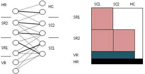
DM and EDM perform an algorithm to obtain a Maximum Matching [8] on the bigraph, identifying the major groups of variables and equations. These groups identify the subsets of variables, which may or may not be determined by solving the system. Fig. 2 describes an example showing the maximum matching and assignment sets, and table 1 expresses the detail of these sets.

Fig. 2.Graphic example of a Maximum Matching and the equivalent partition in the permuted adjacency matrix.

Table 1.Assignment sets for row and column nodes of a matching.

Assignment sets Features

SR1 First set of assigned equations SR2 Second set of assigned equations

VR Redundant equations

HR Equations with indeterminate variables SC1 First set of determinate variables SC2 Second set of determinate variables

HC Indeterminate variables

Increased efficiency by means of this improvement can be justified considering that solving a system of nonlinear equations has a much higher computational cost than solving a linear one.

2.2 Fine Decomposition

Once the variable assignment sets were obtained, the next step is to determine the blocks within the sets SR1-SC1 and SR2-SC2 that will determine the final equations subsystems for the resulting observable variables. To carry out this decomposition, a representation of the sets of rows and columns mentioned by directed graphs or digraphs is used. The Strongly Connected Components De-tection algorithm [11] is applied to the obtained digraphs, which yields the final blocks that determine subsystems of equations assigned to groups of related variables.

A strong component of a digraph is a subset of nodes, with the key feature that any node can be reached from another node within the set, moving through the edges of the digraph. The application of this algorithm in a graph is shown in Fig. 3.

Fig. 3. At the left an example of the strongly connected components detection in a digraph. At the right the structure of a lower triangular block matrix corresponding to the subset SR1-SR2, SC1-SC2 of DM and EDM.

The resolution of each subsystem depends only on the latter, since the new arrangement results in a matrix in Lower Block Triangular Form (see Fig. 3); Therefore, the only variables not yet determined will correspond to the columns in this block and the subsequent ones to the right. The structure resulting from the application of this algorithm to a digraph adjacency matrix is depicted in Fig. 3.

The lower triangular block structure is achieved by applying the permutations in the adjacency matrix, indicated by the algorithms performed to the graph representations. Once this partitioning is done, the system of equations can be easily solved in different stages.

2.3 Simple application example

In this section we show the application of the DM and EDM algorithms to a system of equations. It is shown in Fig. 4. In its associated model, following the given example, it could have been decided that variablesx6,x7andx8are preset with 10, 6 and 8, respectively.

Fig. 4.At the left a system of equations with linear and nonlinear equations. At the right the associated permuted adjacency matrix, obtained by the application of DM and EDM.

The equations that make up this system have different NLD. We can see that equations 1 to 5 contain nonlinear terms, which complicates the resolution of the complete system if it is solved as a unit. By implementing the EDM to partition the main matrix, we obtain the equivalent system partition shown in the adjacency matrix of Fig. 4. If we solve the system step by step according to the blocks identified in Fig. 4, the resolution would involve sequentially process-ing a nonlinear system of 2 equations for x1 and x4, a nonlinear system of an equation for the variablex2, and a nonlinear system of 2 equations for x3 and

3

Convenient partitioning for PSE models

Efficiently solving systems of equations is a topic of interest in various areas of Scientific Computing, because there is a great diversity of models defined by a wide range of systems of varying complexity. The state of the art in numerical optimization shows a revolution in the techniques used to solve a growing range of application problems. There are algorithms with a large theoretical support that make them strong and reliable for its implementation. However, in prac-tice, it is well known that in process-system engineering (PSE) models tend to increase their size and complexity when the formulations evolve towards more realistic designs. Thus, currently it is a great challenge to develop knowledge and refinement of existing software on the design of new algorithms that sup-port higher levels of complexity with minimal computational costs. Therefore, an interesting goal is to develop a module to solve large mixed systems, where a prior matrix reordering is required. Regarding execution times, this tool will efficiently solve complex simulation and optimization problems.

Fig. 5. At the left a decomposition for simulation. At the right a decomposition for optimization.

The EDM obtains a decomposition of the subsystems and an order of prece-dence for the efficient system resolution. It gives excellent results when applied to solving real process monitoring problems. This technique seems to be ex-tremely efficient in terms of execution times, as well as applicable on any kind of matrices, regardless of their structural pattern, increasing its effectiveness as the problems grow in size and complexity. The decomposition technique carried out by the EDM provides a solid basis for developing a methodology that solves large systems of equations.

the algorithm (simulation), while the unobservable variables are in rectangular blocks with more variables than equations (optimization) (see Fig. 5).

4

EDM Algorithm enhancement

The outstanding advantage of EDM with respect to DM is the determination of the NLD of system variables and equations in order to obtain less complex blocks of observable model variables. In its implementation, NLD is included in the maximum matching algorithm, so that when selecting a node to be paired, an adjacent node with the lowest NLD is selected among the feasible ones. The purpose of this paper is to add a step before the determination of the first matching, that conducts a preliminary ascending order of the equations by NLD. The algorithm to obtain a maximum matching used in the above methods including the proposed improvement can be described with the following steps:

1.Sort the adjacent nodes to each node in ascending order by NLD. 2.(Enhancement)Sort the equations set by NLD in ascending order. 3.Build an initial matching with the ordered lists of equations

and adjacent nodes.

4.Find augmenting paths until there are no more paths.

With the first step we ensure that every time we perform a matching, we do this with the least possible NLD in the adjacent node. This principle has already been included in the EDM. The second step is the improvement incorporated in this work. It consists in sorting the system equations based on the NLD of each one. Thus, we also ensure a better sorting because at the time of assembling an initial matching, the first equations that are matched are those with a lower NLD. The first matching obtained is called “Cheap Assignment” [9], and is the basis for the augmenting paths finding process. This process aims at finding an unexplored edge towards an unpaired node that may increase the total amount of nodes in the matching.

4.1 The C language: High Efficiency on Sorting

5

Applications

To verify the performance of the new proposed algorithm, we applied it to two systems of equations with different characteristics: the first is smaller, and is described in Fig. 4, while the second is larger, and comes from a model of a classical distillation column of a chemical plant.

5.1 Application to a small system of equations

The system of equations shown in Fig. 4 exhibits a particular characteristic. Although the equationse1 ande4, taking into account the proposed values for

the variablesx6,x7andx8, form a subsystem of equations that can give us the

values forx1andx4, we see the same situation in the equationse7ande8. Since

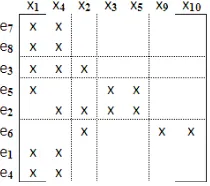
the last two equations above are linear, solving the subsystem that they form is computationally much less expensive than solving the nonlinear one composed of e1 and e4. This issue is not taken into account by the EDM, because of the way it manages the NLD in the equations. When applying this method with the proposed improvement on the arrangement of equations, the result is seen in Fig. 6. Thus, it would be necessary first to solve a linear system, instead of a nonlinear one, in order to determinex1 andx4by using equationse7 ande8.

Fig. 6.Partitioning achieved by applying Enhanced EDM on the example.

This result is an example where an equivalent partition of a system of equa-tions is found, and the resolution may be carried out in a less complex way.

5.2 Application to a system of equations from an equipment model

is performed only for the EDM and the EDM improved, since the basic MD makes no distinction for NLD. The amounts for each type of assignment block are shown in table 2.

Table 2.EDM and Enhanced EDM results for the distillation column example.

EDM Enhanced EDM

Linear blocks of size 1 23 27 Linear blocks of size 3 2 3

Total of linear blocks 25 30 Observable variables 29 36

Nonlinear blocks of size 1 15 11 Nonlinear blocks of size 4 3 2 Nonlinear blocks of size 7 1 0 Nonlinear blocks of size 8 0 1

Total of nonlinear blocks 19 14 Observable variables 34 27 Total of blocks 44 44 Total of observable variables 63 63

From the detail of linear and nonlinear blocks obtained by each algorithm, we can see that with the enhanced EDM more linear blocks are found than with the basic EDM, for this example. EDM identifies 25 linear blocks, while the improved EDM finds 30 and also identifies an additional linear block of size 3. If we calculate the number of variables that are determined in either algorithm based on linear block sizes and quantities, we have that EDM determines 29 variables by linear systems, while the enhanced EDM achieves 36 variables. Following the same reasoning, considering that nonlinear blocks are much more complex to solve, the improved EDM also decreases the total amount of nonlinear blocks from 19 to 14, and the number of nonlinear blocks of size 4 from 3 to 2.

6

Conclusions

We have described the operation of three methods for partitioning adjacency matrices associated with systems of equations from various mathematical mod-els. These methods are based on graph theory to optimize the distribution of equations and variables, so as to facilitate the resolution of such systems. The EDM is based on the DM, and adds the feature of special treatment of variables and equations according to their level of complexity, as measured by NLD. With this method adaptation to the inherent complexity of the system, remarkable progress in optimizing its resolution is made, giving priority to solving simpler subsystems of equations.

algorithm significantly decreases. In the first case a variant in the organization of the adjacency matrix is identified, which consists in the replacement of a sub-system of nonlinear equations by a linear one, with the reduction of processing requirements that it generates. In the second case, we have analyzed the applica-tion of the method to a matrix of a system that is associated with an engineering model of considerable size. The results obtained by the new method overcome those of its predecessor since, among other features, it both increases the amount of linear blocks and at the same time reduces the quantity of nonlinear concomi-tant blocks. This behavior is indicative of a subsconcomi-tantial improvement that the proposed EDM amendment actually offers.

References

1. S. Abbasbandy. Improving newtonraphson method for nonlinear equations by modified adomian decomposition method.Applied Mathematics and Computation, 145(23):887 – 893, 2003.

2. T. B. Benjamin, J. L. Bona, and J. J. Mahony. Model equations for long waves in nonlinear dispersive systems. Philosophical Transactions of the Royal Society of London. Series A, Mathematical and Physical Sciences, 272(1220):47–78, 1972. 3. B. E. Borders. Systems of equations in forest stand modeling. Forest Science,

35(2):548–556, 1989.

4. A. M. Bruckstein, D. L. Donoho, and M. Elad. From sparse solutions of systems of equations to sparse modeling of signals and images. SIAM Rev., 51(1):3481, 2009. 5. A. Domancich.Nuevas Estrategias de Particionamiento para Matrices Ralas Gen-erales: Aplicaciones Matem´aticas y Tecnol´ogicas, Tesis Doctoral en Ingenier´ıa Qu´ımica, Directores: Brignole N.B., Hoch P.A. PhD thesis, UNS, Bah´ıa Blanca, 2009.

6. L. Grigori, P.-Y. David, J. W. Demmel, and S. Peyronnet. Brief announcement: Lower bounds on communication for sparse cholesky factorization of a model prob-lem. InProceedings of the 22nd ACM symposium on Parallelism in algorithms and architectures, SPAA ’10, pages 79–81, New York, NY, USA, 2010. ACM.

7. C. A. R. Hoare. Quicksort. The Computer Journal, 5(1):10–16, 1962.

8. J. Hopcroft and R. Karp. Ann5/2 algorithm for maximum matchings in bipartite graphs. SIAM Journal on Computing, 2(4):225–231, 1973.

9. I. Ponzoni.”Aplicaci´on de Teor´ıa de Grafos al Desarrollo de Algoritmos para Clasi-ficaci´on de Variables”, Tesis Doctoral en Ciencias de la Computaci´on, Directores: Simari G., Brignole N.B. PhD thesis, UNS, Bah´ıa Blanca, 2001.

10. D. A. Spielman and S.-H. Teng. Nearly-linear time algorithms for graph parti-tioning, graph sparsification, and solving linear systems. In Proceedings of the thirty-sixth annual ACM symposium on Theory of computing, STOC ’04, pages 81–90, New York, NY, USA, 2004. ACM.

11. R. Tarjan. Depth-first search and linear graph algorithms. SIAM J. Comput., (1):146–160, 1972.

12. J. Wright, Y. Ma, J. Mairal, G. Sapiro, T. Huang, and S. Yan. Sparse representation for computer vision and pattern recognition. Proceedings of the IEEE, 98(6):1031 –1044, june 2010.