Spatial distribution of R&D expenditure and patent applications across EU regions and its impact on economic cohesion
21
0
0
Texto completo
(2) 03 Martin-Mulas-Granados-Sanz. 42. 5/7/05. 14:36. Página 42. Martín, C., Mulas-Granados, C. y Sanz, I.. minuyeron. De ahí que la conclusión de este artículo sea que la política tecnológica de la UE debe seguir persiguiendo la eficiencia como instrumento de crecimiento económico, al mismo tiempo que destine fondos para proyectos de I+D a las regiones menos desarrolladas para no perjudicar la cohesión. Clasificación JEL: O19, O38, R11. Palabras clave: Política tecnológica europea, cohesión económica, convergencia, indicadores tecnológicos.. 1.. Introducción. The European Union announced in Lisbon 2000 the objective of becoming by 2010 the most competitive knowledge-based economy in the world, and committed itself to undertake all necessary reforms in national and Community policies to achieve this goal. This strategy was based on the firm conviction that government policy can positively affect the long-run growth rate of the economy through economic incentives for the accumulation of various forms of capital and through the promotion of technological innovations. Such a conviction relies on the postulates of endogenous growth models (Romer, 1986 and 1990; Lucas 1988) and has motivated the proliferation of numerous national and European technology programs over the last decades1. The idea behind each of these programs is the following: R&D generates innovation and new technologies, and innovation and new technologies generate then economic growth. This will happen because new technologies increase the productivity of production factors and therefore have a positive supply side effect on the growth potential of the economy. If this linear R&D—Tech/Innovation—Growth mechanism holds, then economic policy authorities would be very interested in promoting innovation and technology through strong R&D programs in the first place. Nevertheless, the relative success of these programs in achieving real innovation, and the relative success of these inventions in effectively generating higher rates of economic growth is still a matter of debate. The question of whether technology policies have really had any significant role in promoting economic growth or improving economic cohesion, still needs to be answered. Note, however, that the resolution of such research question would imply the development of a qualitative study based on the description of different policy initiatives which would complicate enormously 1. s -. While neo-classical growth models (Solow, 1956; Mankiw, Romer and Weil, 1992) consider that economic integration would assure convergence between poor and rich countries (regions) due to capital accumulation in poorer regions that present higher returns to capital, more sophisticated endogenous growth models (Romer, 1986 and 1990; Lucas 1988) and new economic geography models (Krugman, 1991; Ottaviano and Puga, 1998) show that income convergence need not occur as a result of economic integration. Consequently, pro-active public policy has a role to play in the promotion of economic convergence between poorer and richer countries or regions. For a more detailed summary of growth theories and the convergence-divergence debate, see Martin and Sanz (2003)..
(3) 03 Martin-Mulas-Granados-Sanz. 5/7/05. 14:36. Página 43. Spatial distribution of R&D expenditure and patent applications across EU regions and its.... 43. the attribution of causality relationships between technology policies and economic performance. Instead, a better strategy is to study the evolution of some important technology indicators (mainly R&D spending and patent applications), assuming that there exists a connection between technology policies and technology outcomes in terms of R&D spending and patent applications. By doing this, a systematic quantitative analysis can be developed. The research question could then be reformulated as follows: Have R&D spending and patent applications had any positive or negative effect on economic growth and cohesion? This is the question that this paper will answer, and in doing so, the article not only wants to contribute to the debate on technology and growth, but also wants to investigate the possible existence of a trade off between economic growth and economic cohesion mediated by technology policies in general, and by technology indicators in particular. Aware of the likely existence of this trade off, Community policies have combined until now economic growth initiatives —such as R&D and technology programs— and explicit actions for economic cohesion —mainly through the structural funds— (Peterson and Sharp, 1998 and Pavitt, 1998). Now that these policies are being questioned in the current debate for the reorganization of European funds and policies it is crucial to link the answer of the research question that motivates this paper to the possible existence of the mentioned trade off. In order to do this, section 2 studies the spatial distribution of technology indicators over the last decade. Since the main finding of this section is that regional government R&D spending has converged while total R&D spending has diverged over the last decade, section 3 and section 4 focus on the likely different effect that these two R&D indicators may have had on economic performance. Therefore, section 3 re-interprets the evolution of these technology indicators vis á vis economic cohesion, and section 4 replicates the analysis for economic growth. Finally section 5 recapitulates and concludes.. 2.. Spatial distribution of technology indicators over the last decade. Technology policies are very difficult to measure quantitatively, and therefore their analysis has to rely on a set of technology indicators that approximate different phases of these policies, assuming that they follow a certain input-output sequence. Following the trend in the specialized literature we use total R&D expenditures by all sectors in % of GDP (TERD) as the best technology input indicator. The idea that total expenditures in R&D is a good indicator of technological innovation is basically derived from the so-called linear model of innovation2, which assumes that investment in basic research is strongly positively correlated with technological innovation in the market place. Independently of whether this assumption holds or not, this is the best indicator to have an idea of the resource allocation to R&D in a particular region. 2. For a summary, see Soete and Arundel (1993)..
(4) 03 Martin-Mulas-Granados-Sanz. 44. 5/7/05. 14:36. Página 44. Martín, C., Mulas-Granados, C. y Sanz, I.. As an indicator of technology output we take the number of patent applications per million people. This is the so-called «inventiveness coefficient» and should be interpreted with care since Southern European regions are much less inclined to fill in patents for innovative products of processes (European Commission, 1997: 349). In spite of this fact, this is the best indicator to give an idea of the technology output intensity in a particular region3. Finally, because we want to analyze separately if publicly finance policies have a different relative impact than the previous standard technology indicators, we analyze separately the evolution of government R&D expenditures (GERD), which is in itself a portion of the more general total R&D spending by all sectors4. The use that we make in this section of all these indicators is twofold: first we just describe their spatial and temporal evolution, and then we report the results of a systematic convergence analysis whereby the common measures of economic and technological convergence are calculated and reported. In this respect, although in the specialized literature there is an open debate on the relative merits of different convergence measures5, the two most popular measures are: the beta-convergence and the sigma-convergence. The former implies that the poor countries (regions) grow faster than the richer ones and it is generally tested by regressing the growth in per capita GDP on its initial level for a given cross-section of countries (regions). In turn, this beta-convergence covers two types of convergence: absolute and conditional (on a factor or a set of factors in addition to the initial level of per capita GDP). Under sigma-convergence we mean the reduction of per capita GDP dispersion within a sample of countries (regions) (see Barro and Sala-i-Martin (1995:11) for further details). We begin with the simplest indicator of all: the absolute beta-convergence index. Xie, Zou, and Davoodi (1999) elaborate a endogenous growth model based on Barro (1990) and Devarajan, Swaroop, and Zou (1996), where the production function has private capital and different components of government spending. Assuming a Cobb-Douglas production function, these authors obtain that the growth-maximizing share of a component of government expenditure in total government expenditures is equal to its elasticity divided by the sum of elasticities of all the components. Following this model, Sanz and Velazquez (2004) show that if output elasticities with respect to each component of government expenditure are similar across countries and that governments maximize growth, we should expect convergence in the composition of government expenditures among countries. Thus, as long as the elasticity of growth with respect to public R&D spending is similar across countries, we should expect convergence across public R&D 3. Data for all technology and economic indicators used in this paper comes from the New Chronos database of the European Commission. For R&D expenditures at regional level data presents a significant number of gaps for Belgium, Ireland, the Netherlands, Sweden and the UK between 1989 and 1994. Where possible gaps in the patents and R&D data have been filled out by means of simple estimation techniques. In the case of the Innovation Index, data is only available for year 2002 and has been obtained from the 2nd European Scoreboard on Innovation (2002). 4 The other sectors being private R&D spending and R&D spending by higher education institutions. 5 For references on this debate, see Baumol, Nelson and Wolff (1994); Barro and Sala-i-Martin (1995); Quah (1993, 1996); and Boyle and McCarthy (1997, 1999)..
(5) 03 Martin-Mulas-Granados-Sanz. 5/7/05. 14:36. Página 45. Spatial distribution of R&D expenditure and patent applications across EU regions and its.... 45. spending in EU countries. Indeed, Gemmell and Kneller (2002) show that long-run growth elasticity of productive expenditures exhibit a high degree of uniformity across OECD countries. We start with the examination of β convergence, with the object of evaluating whether regions that have a higher public R&D spending increase (decrease) this percentage to a lesser (greater) extent than regions in which public R&D spending is lower. We will also adapt this analysis to aggregate R&D spending and patents in order to evaluate whether regions in which aggregate R&D spending and patents are lower have higher rates of growth. In this way we will be able to compare convergence in public R&D spending with aggregate R&D spending and patents. For this purpose we use the well-known ‘Barro type regression’: In (TIit) – In (TIi,t–1) = αi + β In (TIi,t–1) + εit. [1]. where: TIt: is the Technology Indicator (patents, R&D, etc.) in year t. i: 205 regions of the EU at the NUTS II level of disaggregation for regional convergence t: all the years in the period 1989-2000 α: regional dummy. β: coefficient reflecting the existence and the speed of convergence. According to this equation, if the coefficient β takes a negative and significant value, there has been a convergence process in this technology indicator. Also, there would be absolute convergence in two cases: firstly if the GLS estimator is unbiased and hence we do not include any other variable apart from the previous year’s value as an explanatory variable for the change of rate; and secondly if only the within estimator is unbiased, but we can not reject the hypothesis of country dummies being equal for all the regions (De la Fuente, 2000). In this case all the regions will converge to the same steady state. Then, because the existence of beta-convergence is a necessary but not sufficient condition for convergence (Barro and Sala-i-Martin, 1992), we also compute the standard deviation of the logarithm of each technology indicator. In this context, the sigma-convergence explores if the dispersion among the different measures of technology inputs or outputs among European regions has been reduced. Finally, to complement and illustrate the results provided by the beta-convergence and sigmaconvergence analyses, we also plot Tukey’s box-and whisker plots for all technology indicators under study. The Tukey’s box-and-whisker plot is a histogram-like method of displaying data, where the box ends at the quartiles Q1 and Q3, and the statistical median is represented by a line that crosses the box. The farthest points that are not outliers (i.e. that are within 3/2 times the interquartile range of Q1 and Q3) are connected to the box by the «whiskers», and for every point that is more than 3/2 further away the end of the box, we draw a dot. To put the previous spatial distribution of total R&D expenditures in context, it is very important to note that statistics at the regional level show the more severe.
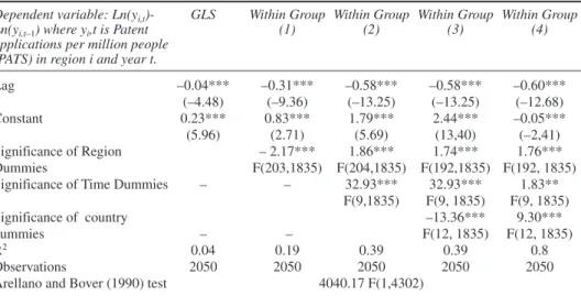
(6) 03 Martin-Mulas-Granados-Sanz. 46. 5/7/05. 14:36. Página 46. Martín, C., Mulas-Granados, C. y Sanz, I.. disparities between regions that remain hidden in statistics at national level. This is specially true for data on technology indicators. For example, disparities in technology input (TERD/GDP) and output (patents per million people) are as much as 20 and 55 times respectively higher at regional than at the national level. If one looks at the distribution of European regions that invested most in total R&D (as % of GDP) in 2000, we observe important disparities. Among the regions that invested most we find Braunschweig (7.19%), Stuttgart (4.92%), Oberbayern (4.79%), Pohjois-Suomi (4.73%); Pohjois Suomi (4.73%), Uusimaa (4.09%) and Tübingen (4.31%). And among the regions that invested least we find Calabria (0.24%), Castilla-la Mancha (0.22%), Sterea (0.18%), Dykiti Makedonia (0.07%) and Notio Aigaio (0.06%). In 2000, the EU’s average regional R&D spending was 1.22% of GDP with a 1.01 standard deviation. The spatial distribution of patent applications presents more disparities across regions than the distribution of total R&D expenditures. There are many regions which in 2000 filled out less than 4 patent applications per million people. Among them we find for example, Dessau (3.3), Andalusia (2.8), Molise (1.9), Galicia (1.5) or Calabria (0.9). On the opposite side, there were many regions which filled out more than 180 applications per million people. These were the cases of Koln (189.3), Berkshire (197.1), Stockholm (219.7), Noord-Brabant (266.8), Darmstadt (306.6) and Oberbayern (441.95), among others. Such a degree of disparity placed the EU’s average of patent applications per million people at regional level in 152.8, with a standard deviation of 147.9 in year 2000. It is worth noting that once controlled for the outliers, the regional disparity in technological development is not so high. This is because patenting activity is Europe is dominated by a small set of regions (an «Archipielago» of ten regions as suggested by Hilpert (1992)), with all others making only a marginal contribution. When compared to the spatial distributions of the two previous technology indicators, the regional distribution of public R&D (as % of GDP) is less dispersed. While there is a group of regions with very low levels of public R&D spending that range between 0.01 and the 0.04 of the region’s GDP (Schwaben, Sterea Ellada, Oberfranken, Koblenz, Rioja and Voralberg), there is another group that spends more public funds in R&D but at a moderate distance (Berlin 1.1%, MidiPyrénées 1.46% and Flevoland 1.87%). In 2000 the average level of EU’s regional public R&D spending remained at 0.19% of GDP with a standard deviation of 0.27. In view of the situation that technology indicators presented by the end of 2000, the question is now whether the spatial distribution of these indicators converged, diverged or remained intact along the last decade. In first place, Arellano and Bover (1990) test show that there are significant individual effects (see tables 1-3)6. There has been conditional convergence in R&d figures and in patent applications. This overall convergence has been, however, stronger in terms of patent applications than in total R&D 6. Arellano and Bover (1990) test consists in comparing the coefficients in levels and first differences, so that if these are different the hypothesis of absence of correlation between unobservable effects and explanatory variables is rejected, which would mean the existence of significant individual effects..
(7) 03 Martin-Mulas-Granados-Sanz. 5/7/05. 14:36. Página 47. Spatial distribution of R&D expenditure and patent applications across EU regions and its.... 47. expenditures7. As the different coefficients in tables 1-3 show, the same has occurred with government R&D expenditures which have converged at a higher speed than any other technology indicator. It should be pointed out, however, that the results obtained in column 2 of tables 1-3 may be biased by the ‘country effect’, i.e.: by the fact that technology is more affected by the development of the country to which regions belong than by the actual features of the region. Consequently, we proceed in two ways to confirm that there has been regional convergence. First, in equation (3) we estimate convergence for the 205 regions including a dummy for the 15 Member States that takes value 1 if the region belong to a particular country and 0 if otherwise. Thus, we reduce the spatial self-correlation caused by the fact of the regions belonging to the same geographical areas (Armstrong, 1995). In this way, we obtain the results very similar to column (2) in all the tables. Second, in equation (4) we estimate regional convergence but taking the regional technological indicators in relation to the country average to which each region belongs. By means of this procedure, similar to that used in Rodríguez-Pose (1996), a very similar estimate to column (2) and (3) is obtained. Hence, from both procedures, it may be verified that, apart from the ‘country effect’ there is a technological convergent tendency specific of the regions. Furthermore, results corroborate that convergence in public R&D spending is higher than in aggregate government R&D spending. In fact, the different path of convergence of total and government R&D over the 1990-2000 period intensified during the second half of the nineties up to a point where regional total R&D expenditures started to diverge. This progressive divergence between both measures of R&D spending probably reflects the impact of the rapid expansion of private R&D spending as a share of total R&D expenditures. During the second half of the nineties while private R&D investment boosted, public R&D expenditures remained frozen at constant levels under the influence of general framework of budget stability. The sigma-convergence analysis reports very similar results to those provided by the previous beta-convergence analysis with only one exception (see figure 1). While both the beta and sigma-convergence analyses point to a convergence in patent applications and public R&D expenditures, particularly strong between 1996 and 2000, the picture for the evolution of total R&D expenditures is more heterogeneous. Apparently there exists beta-convergence and sigma-divergence over time. The existence of beta convergence would mean that regions with lower shares of total R&D in 1990 have increased their R&D expenditures at higher rates than those regions which started at higher levels. At the same time, the existence of sigma-divergence would imply that the dispersion from the average share of total R&D spending has increased. Ne7. Note, however, that data on patent applications does not discriminate for the nationality of the company or the university where the innovation to be patented was produced. Therefore multinationals from big advanced economies may be producing innovations that belong to them, but are filling in the patents in the country where they are going to use that new technology. Many of the current convergence in patent applications only responds to this process. The nationality of the “inventors” may remain the same, while the distribution of patents applications becomes more equally distributed across regions only as result of the expansion of these multinationals. Unfortunately it is impossible to discount the share of this effect from the data that we have..
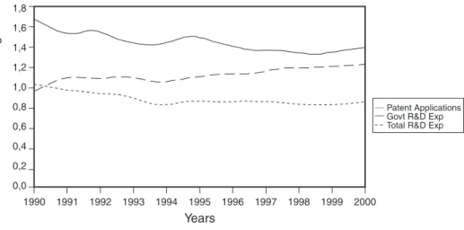
(8) 03 Martin-Mulas-Granados-Sanz. 48. 14:36. Página 48. Martín, C., Mulas-Granados, C. y Sanz, I.. Figure 1.. Standard Deviation of the Logarithms. 5/7/05. Sigma Convergence of Technlogy Indicators among EU Regions (1990-2000). 1,8 1,6 1,4 1,2 1,0 0,8. Patent Applications Govt R&D Exp Total R&D Exp. 0,6 0,4 0,2 0,0 1990. 1991. 1992. 1993. 1994. 1995. 1996. 1997. 1998. 1999. 2000. Years. vertheless, these two results are not incompatible, because the existence of beta–convergence is a necessary but not a sufficient condition for sigma-convergence (De la Fuente, 2000). Random shocks may have increased temporarily the dispersion of total R&D expenditures even in the presence of beta-convergence or regions may be approaching their steady state shares (conditional convergence) with higher dispersion than at the beginning of the period. In addition, evidence of beta-convergence may be reflecting Galton’s fallacy, i.e. the tendency for regions to regress towards the mean (Quah, 1993). Just by looking at figure 1 it is easy to arrive at a very interesting finding: at the beginning of the nineties the fact of measuring the technological gap using different indicators really made a difference. In 1990, the existing technological gap measured by the sigma in patent applications (1.6) was twice the technological gap if the indicator to be used was total R&D expenditures (0.8). In 2000 the technological gap that both indicators measure is much closer, since in that year the sigma for patent applications was 1.6 while the sigma for total R&D expenditures was 1.3. Finally, all the dynamic evolution of the different distributions under study that was described in previous paragraphs is confirmed again when the three Tukey’s box and whisker figures are plotted. As can be seen in the first plot of figure 2, average total R&D spending has increased along time, as well as its degree of dispersion. However, the average level of public R&D has remained almost constant along the past decade and so has its degree of dispersion (plot 2). Finally, the average number of the log of patent applications has increased slightly in the last decade, while its dispersion diminished specially in 1995 and again in 2000. It is interesting to analyze the shape of the different Tukey’s box plots because they offer some new information on the sources of the existing disparities in the distribution of each technology indicator. The fact that dots are above the upper whiskers in the plots for total and public R&D.
(9) 03 Martin-Mulas-Granados-Sanz. 5/7/05. 14:36. Página 49. Spatial distribution of R&D expenditure and patent applications across EU regions and its.... Figure 2.. Tukey’s box and whisker plots of Total R&D (TERD), Government R&D (GERD) and Patent Applications (PATS), 1989-2000. Total Expenditure in R&D 7.195. .02 1989. 1990. 1991. 1992. 1993. 1994. 1995. 1996. 1997. 1998. 1999. 2000. Goverrnment Expenditure in R&D 3.075. 0 1989. 1990. 1991. 1992. 1993. 1994. 1995. 1996. 1997. 1998. 1999. 2000. Patent Applications 6.64197. 1.79677 1989. 1990. 1991. 1992. 1993. 1994. 1995. 1996. 1997. 1998. 1999. 2000. 49.
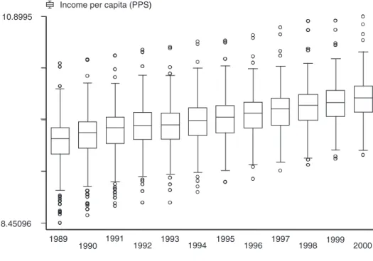
(10) 03 Martin-Mulas-Granados-Sanz. 50. 5/7/05. 14:36. Página 50. Martín, C., Mulas-Granados, C. y Sanz, I.. expenditures implies that most regional disparities in R&D expenditures originate in regions that clearly spend long above the regional average. On the contrary the problem with patent applications is exactly the opposite: there is a significant number of regions that fill in very few patent applications and are therefore way below the regional average. Interestingly enough, and as we will see in next section (figure 4), income disparities seem to be somewhat in between and find their roots in the existence of both very rich and very poor regions. Summing up the results reported until now, the most striking finding that the convergence analysis has provided is the empirical evidence showing that public and total spending in R&D have followed different dynamics over the last decades. If this different evolution has been translated into a different impact on economic cohesion and growth is the subject of the two following sections.. 3. Spatial distribution of technology indicators vis á vis Economic Cohesion This section turns now, therefore, to explore the relationship between technology policy and economic performance. Following a logic structure we focus first on the link between the spatial distribution of technology indicators and the spatial distribution of income across European regions (also known as regional economic cohesion). Before this analysis can proceed it is necessary to briefly describe the evolution of the distribution of regional income per capita during the same period. As can be observed in table 4 and figures 3 and 4, both beta and sigma convergence measures, together with the evolution of the corresponding Tukey’s box plot, point in the direction of an important convergence in the distribution of income per capita at regional level in Europe. If the beta coefficients in table 4 are compared to those in tables 1-3, we see that convergence in income per capita has been weaker than convergence in some technology indicators. In addition, as figure 3 shows, the main reduction in regional income disparities occurred at the beginning of the nineties, and this process remained stagnated around similar levels during the rest of the decade. Finally, on the Tukey’s box plot of figure 4, using the log of per capita income, we can observe that the number of dots under the bottom whiskers has been progressively reduced along the nineties, what implies that the reduction of income disparities across regions has been mainly based on the convergence of poorer regions to the EU average. Since we have assumed along the paper that there exists economic cohesion when the regional dispersion in GDP per capita diminishes, we want to estimate the relative impact that changes in the regional dispersion of technology indicators have on the regional dispersion of income per capita. To do so, we estimate the following equation, where all dependent and independent variables are transformed into their sigmadispersion indexes. SigmaINCOME = SigmaPATENTS + SigmaTERD + SigmaGERD + ε. [2].
(11) 03 Martin-Mulas-Granados-Sanz. 5/7/05. 14:36. Página 51. Spatial distribution of R&D expenditure and patent applications across EU regions and its.... Standard Deviation of the Logarithms. Figure 3.. 51. Sigma Convergence in the Distribution of Income per capita among EU Regions (1990-2000).. 0,4. 0,3. Income per capita. 0,2. 0,1. 1990. 1991. 1992. 1993. 1994. 1995. 1996. 1997. 1998. 1999. 2000. Years. Figure 4.. Tukey’s box and whisker plot of Income per capita, 1990-2000. Income per capita (PPS) 10.8995. 8.45096 1989. 1990. 1991. 1992. 1993. 1994. 1995. 1996. 1997. 1998. 1999. 2000. The equation is estimated by OLS and all results are reported in table 5. These results show that any increase in the dispersion of total R&D spending or in the dispersion of patent applications increases the dispersion in the income distribution among.
(12) 03 Martin-Mulas-Granados-Sanz. 52. 5/7/05. 14:36. Página 52. Martín, C., Mulas-Granados, C. y Sanz, I.. regions in all EU and among regions by country. The influence of public R&D spending on economic cohesion is weaker8 but works in a similar direction. This direct relationship between the dispersion in all technology indicators and the dispersion in income per capita can be re-interpreted in view of the actual evolution of each indicator along the nineties that was portrayed in section 2 of this paper (see figure 1 and table 5). A 10% increase in the dispersion of total R&D expenditures as the one occurred between 1998 and 2000, produced a 0.3% increase in the dispersion of income distribution across regions in Europe. On the other hand, a 10% decrease in the dispersion of public R&D expenditures as the one occurred between 1993 and 1995 and again between 1997 and 1999 produced each time a reduction of 0.1% in the income dispersion across regions in Europe. Apparently, the experience of the nineties shows that while the distribution of total R&D spending became more unequal (led by an unequal expansion of its private component) the only reason why this did not turn into a more unequal distribution of income per capita was due to the compensating effect performed by public R&D spending and patent applications. As the distribution of patents and public R&D converged, income per capita converged too. Since the only indicator that can be directly affected by policy-makers is the share of public funds that they dedicate to R&D activities, it looks like the government R&D has been used purposefully and successfully along the nineties to reduce the economic disparities that other technology indicators promoted. Whether this «cohesive» role played by public R&D expenditures has had any damaging impact on the rate of economic growth of these regions is a question that remains for the final section.. 4. Spatial distribution of technology indicators vis á vis Economic Growth There is a long tradition of empirical and theoretical studies on the role that technology plays on economic growth. While some recent works have found that economic convergence depends on a set of factors among which technology is only one of them (Paci, 1997; Dunford and Smith, 2000; Tondl, 2001), others have emphasized the decisive role that technology plays for long run economic convergence (Fagerberg, Verspagen and Caniels, 1997; Paci and Usai, 2000; and Paci and Pigliaru, 2001)9. In order to study the relationship between the three technology indicators and economic growth this final section proceeds as follows: first, we simply study the correlation between the three technology indicators and income per capita. Then, we present the results of a multiple regression for the impact of technology on economic growth (measured as the annual change in GDP per capita). The correlation analysis provides clear-cut findings. As table 6 shows the correlations between income per capita and patents applications are very strong (0.7) and persistent over time. The same occurs with the correlations between income per capita and total R&D spending 8 9. Coefficients for public R&D spending are only statistically significant at the 80% confidence level. For a critical essay on the growth literature see Fagerberg (2000)..
(13) 03 Martin-Mulas-Granados-Sanz. 5/7/05. 14:36. Página 53. Spatial distribution of R&D expenditure and patent applications across EU regions and its.... 53. (0.4). On the contrary, the correlations between income per capita and public spending in R&D are much weaker (0.15) and dilute over time. The joint role that all those technology indicators have in explaining economic growth measured by the annual change in income per capita can be discerned by estimating the following equation10: ∆GDPit = α0 + βo (GDPli,t–1) + β1 (TIfi,t–1) + βg (TIgi *cohesiongi,t–1) + [3] + δt + ωp + øi + εti where: ∆GDPit: is the annual change in income per capita β1: is the coefficient reflecting the effect that all technology indicators (patent applications, total R&D spending, and public R&D spending) have on regional economic growth. βg: is the coefficient reflecting the effect that all technology indicators (patent applications, total R&D spending, and public R&D spending) have in regional economic growth in cohesion countries (Spain, Greece, Ireland and Portugal). The reason for including an interaction for the group of cohesion countries is that the relation between technology and growth might be different for different clusters (Clarysse and Muldur, 1999: 4)11. Clearly cohesion countries share common initial conditions and in this respect they can be considered as a separate cluster. δt: is the time dummy; øi: is the region dummy; ωp: is the country dummy. Note that growth might influence R&D spending decisions of both the business sector and the government. Growth increases government revenues, which in turn would raise the resources allocated to R&D spending. Companies in countries recording high growth rates may also devote more funds to R&D activities. For this reason, we introduce the lag values of the independent variables. In fact, regression (3) resembles the Beck and Katz´s dynamic model (1995, 1996 and 2005). Indeed, estimating equation (3) yields the same results as estimating GDP on its lagged value and independent variables. Thus, we are capturing long-term relationship between GDP and patents, aggregate R&D spending and government R&D spending. Moreover, endogeinity is not an issue anymore, as long as there is not first order autocorrelation in the error term (Beck and Katz, 1996). In the absence of first order autocorrelation, the error term will not be correlated with independent variables. Furthermore, Beck and Katz (1996) claim that «If the errors show serial correlation in the presence of a lagged dependent variable, the standard estimation strategy is instrumental variables. While this has fine asymptotic properties, it may perform very poorly in practical research situations (...) Thus it may well be the case that it is better to estimate with OLS, even in 10 We accept that one limitation of a cross-sectional analysis as the one we perform here is that, despite the fact that it is directly derived from the traditional neoclassical model, it does not test the validity of this model against alternative and conflicting ones (Magrini, 2004). Nonetheless, since the objective of this study is to test the role of technology on economic convergence, and not to discern among different convergence theories, we decided to follow the most common and simplest formulation to perform the empirical analysis. 11 See Quah (1996); Neven and Gouyette (1995) or Fagerberg and Verspagen (1996)..
(14) 03 Martin-Mulas-Granados-Sanz. 54. 5/7/05. 14:36. Página 54. Martín, C., Mulas-Granados, C. y Sanz, I.. the presence of a small, but statistically significant, level of residual serial correlation of the errors». This is our case, The Lagrange Multiplier test shows that lagged residuals are marginally significant in predicting residuals from equation (3). Therefore, equation (3) is estimated through GLS with robust standard errors. Results are reported in table 7. As can be observed, real convergence is once again confirmed: the lower the existing regional income per capita in t-1, the higher the subsequent economic growth. In addition, the contribution of patent applications in t-1 to subsequent economic growth in year t is very positive. An increase of 1% in patent applications produces an increase in regional economic growth of 0.017. However, this effect is not so strong for cohesion countries. This can be interpreted as follows: where the stock of patents is very low, one additional patent is not sufficient to start economic growth. Instead, the innovative effort required to produce an isolated patent could diverting resources from more productive activities. More importantly, the role of total R&D expenditures is also strongly positive for all countries (including cohesion ones). The crucial impact of total R&D for economic growth is somewhat at odds with the insignificant effect that public R&D spending has on economic performance. However, this weak (even negative) short run impact of public R&D on economic growth, turns into a very strong and positive influence in the medium run. An increase of 1% in public R&D spending today is likely to increase the rate of growth by 0.04% in four years from now12. This 4-years lagged positive effect of public R&D on economic growth holds also for cohesion countries, what is very important given the fact that public R&D spending has to compensate for the low presence of private R&D initiatives in these regions.. Conclusion The study of the evolution that the distribution of regional technology indicators has experienced over the last decade has provided some clear and important findings which can be very useful to inform future economic policy debates in the EU. First of all, some technology indicators have converged among regions during the nineties (especially public R&D spending), and this has ran parallel to a real (though softer) convergence in income per capita levels. On the contrary total R&D expenditures have diverged across regions over time, as a result of an asymmetric expansion of private R&D activities during the second half of the nineties. Secondly, we have seen that total R&D spending increases economic growth, especially if this R&D activity is quickly transformed into new patent applications. Since innovation is the real key for economic growth, only when efficient total R&D allocations are easily transformed into new patent applications, economic performance improves. This positive effect on growth is not exclusive of total R&D expenditures, but also applies with a 4-year delay to public R&D initiatives. Finally and most importantly, in addition to this lagged positive effect on growth, 12. The four lagged public R&D expenditure shows the highest impact on economic growth. Further lagged values seem to have also impact on economic growth but to a lesser extent..
(15) 03 Martin-Mulas-Granados-Sanz. 5/7/05. 14:36. Página 55. Spatial distribution of R&D expenditure and patent applications across EU regions and its.... 55. government R&D spending has also demonstrated to be closely associated to regional economic cohesion in the short and medium run. When the dispersion of public R&D across regions diminished in the second half of the nineties, income disparities at regional level also decreased. Therefore, while technology policy based on pure excellence and efficiency criteria should remain as a policy tool for economic growth, this policy should be counterbalanced by European and regional policies which transfer funds to the least developed regions to maintain a minimum degree of economic cohesion. The results shown in this paper clearly demonstrate that if the current winds of reform succeed in curtailing the public financing of technology policies, the degree of regional polarization in the EU will most likely increase in the future.. References Armstrong, H.W. 1995: An appraisal of the evidence from cross-sectional analysis of the regional growth process within the European Union, in H.W. Armstong and R.W. Vickerman (eds.): Convergence and Divergence among European Regions, Pion, Londres. Barro, R.J. 1990: Government spending in a simple model of endogenous growth. Journal of Political Economy 98: S103-125. Arellano, A. and Bover, O. 1990: La Econometría de Datos de Panel, Investigaciones Económicas 14, 345. Barro, R. and Sala-i-Martin, X. 1992: Convergence, Journal of Political Economy 100, 223-51. Beck, N. and Katz, J.N. 1995: What to Do (and Not to Do) with Time-Series-Cross-Section Data, American Political Science Review, Vol. 89: 634-947. Beck, N. and Katz, J.N. 1996: Nuisance vs. Substance: Specifying and Estimating Time-Series-CrossSection Models, Political Analysis, Vol. VI: 1-36. Beck, N. and Katz, J.N. 2005: The Analysis of Time-Series—Cross-Section Data Michigan: University of Michigan Press, forthcoming. Boyle, G.E. and McCarthy, T.G. 1997: A Simple Measure of b-convergence, Oxford Bulletin of Economics and Statistics 59, 257-264. Boyle, G.E. and McCarthy, T.G. 1999: Simple Measures of Convergence in per Capital GDP: a Note on Some Further International Evidence, Applied Economics Letters 6, 343-347. Baumol, W.J., Nelson, R.R. and Wolff, E.N. 1994: Introduction: The Convergence of Productivity, Its Significance, and Its Varied Connotations, in: W.J. Baumol, R. Nelson and E.N. Wolff (Editors) Convergence of Productivity (Oxford University Press, Oxford), 3-19. Clarysse, B. and Muldur, U. 1999: Regional Cohesion in Europe? An Analysis of How EU Public RTD Support Influences the Techno-Economic Regional Landscape, (European Commission, Brussels). De la Fuente, A. 2000: Convergence across countries and regions: theory and empirics, CEPR Discussion Paper Series 2465. Devarajan, S., Swaroop, V. and Zou, H. 1996: The composition of public expenditure and economic growth. Journal of Monetary Economics 37: 313-344. Dunford, M. and Smith, A. 2000: Catching-up or Falling Behind? Economic Performance and Regional Trajectories in the New Europe, Economic Geography 76, 2, 169-195. European Commission. 1997: 2nd European Report on Science and Technology Indicators, (European Commission, Brussels). European Commission 2002: 2nd European Scoreboard on Innovation, (European Commission, Brussels). European Commission. 2003: 3rd European Report on Science and Technology Indicators, (European Commission, Brussels)..
(16) 03 Martin-Mulas-Granados-Sanz. 56. 5/7/05. 14:36. Página 56. Martín, C., Mulas-Granados, C. y Sanz, I.. Fagerberg, J. 2000: Vision and Fact. A Critical Essay on the Growth Literature, in: J. Madrick (Editor), Unconventional Wisdom: Alternative Perspectives on the New Economy (The Century Foundation Press, London). Fagerberg, J. and Verspagen B. 1996: Heading for Divergence? Regional Growth in Europe Reconsidered, Journal of Common Market Studies 34, 431-448. Fagerberg, J., Verpagen, B. And Caniels, M.C.J. 1997: Technology Gaps, Growth and Unemployment Across European Regions, Regional Studies 31, 5, 457-466. Gemmell, N. and Kneller, R. 2002: Fiscal policy, growth and convergence in Europe. European Economy Group Working Paper No. 14. Hilpert, U. 1992: Archipelago Europe: Islands of Innovation. Synthesis Report, (European Commission, Brussels). Krugman, P. 1991: Geography and Trade, (MIT Press, Cambridge). Lucas, R.E. 1988: On the Mechanics of Economic Development, Journal of Monetary Economics 22, 3-42. Magrini, S. 2004: Regional (Di)Convergence, in: V. Henderson and J.F. Thisse (Editors), Handbook of Urban Economics (Elsevier Science Publishers, London). Mankiw, G.N., Romer, D. and Weil D.N. 1992: A Contribution to the Empirics of Economic Growth, Quarterly Journal of Economics 107, 407-437. Martin, C. and Sanz I. 2003: Real Convergence and European Integration: The Experience of the Less Developed EU Members, Empirica 30, 205-236. Muñoz, E. 2001: The Spanish system of research: Research and innovation in Spain, in: P. Laredo and P. Mustar, (Editors) Research and innovation policies in the new global economy: an international comparative analysis, (Edward Elgar: Cheltenham), 359-397. Neven, D.J., and Gouyette, C. 1995: Regional convergence in the European Community, Journal of Common Market Studies 33, 47-65. Ottaviano, G. and Puga, D. 1998: Agglomeration in the Global Economy: A Survey of the New Economic Geography, World Economy 21, 707-731. Paci, R. 1997: More Similar and Less Equal: Economic Growth in the European Regions, Weltwirtschaftliches Archiv 133, 609-634. Paci, R. and Pigliaru, F. 2001: Technological Diffusion, Spatial Spillovers and Regional Convergence in Europe, CRENOS Working Paper No. 1/01. Paci, R. and Usai, S. 2000: Technological Enclaves and Industrial Districts. An Analysis of the Regional Distribution of Innovative Activity in Europe, Regional Studies 34, 97-104. Pavitt, K.1998: The inevitable limits of EU R&D funding, Research Policy 27, 559-568. Peterson, J., and Sharp M. 1998: Technology Policy in the European Union, (Macmillan Press, London). Quah, D.T. 1993: Galton’s Fallacy and Tests of the Convergence Hypothesis, Scandinavian Journal of Economics 95, 427-43. Quah, D.T. 1996: Convergence Empirics Across Economies with Some Capital Mobility, Journal of Economic Growth 1, 95-124. Rodríguez-Pose, A. 1996: The socio-political bases of regional growth in Western Europe, PhD Thesis, European University Institute, Florence. Romer, P.M. 1986: Increasing returns and long run growth, Journal of Political Economy 94, 1002-1037. Romer, P.M. 1990: Endogenous Technological Change, Journal of Political Economy 98, 5-21. Sala-i-Martin, X. 1995: Regional Cohesion: Evidence and Theories of Regional Growth and Convergence, CEPR Discussion Paper 1075. Sanz, I and Velázquez, F.J. 2004: The Evolution and Convergence of the Government Expenditure Composition in the OECD Countries, Public Choice, 119: 61-72. Soete, L. and Arundel A. (Editors). 1993: An Integrated Approach to European Innovation and Technology Diffusion Policy: A Maastricht Memorandum, (European Commission, Brussels).. Solow, R.M. 1956: A Contribution to the Theory of Economic Growth, Quarterly Journal of Economics 70, 65-94. Tondl, G. 2001: Convergence After Divergence? Regional Growth in Europe, (Springer, Wien). Xie, D., Zou, H. and Davoodi, H. 1999: Fiscal decentralization and economic growth in the United States. Journal of Urban Economics 45: 228-239..
(17) 03 Martin-Mulas-Granados-Sanz. 5/7/05. 14:36. Página 57. Spatial distribution of R&D expenditure and patent applications across EU regions and its.... 57. Anexo Table 1.. β-convergence of the distribution of Total R&D Expenditure among EU Regions (1990-2000).. Dependent variable: Ln(yi,t)Ln(yi,t–1) where yi,t is Total R&D Expenditure as a % of GDP (TERD) in region i and year t.. GLS. Lag. –0.16*** (–8.85) Constant –0.38*** (–8.31) Significance of Region Dummies – Significance of Time Dummies. –. Significance of country dummies. –. R2 Observations Arellano and Bover (1990) test. 0.082 1487. Within Group Within Group Within Group Within Group (1) (2) (3) (4)a. –0.41*** –0.41*** (–6.93) (–6.91) –1.97*** –1.97*** (–7.07) (–7.08) 3.30*** 3.06*** F(151, 1078) F(151, 1068) – 0.91 F(10, 1068) – – 0.284 1234. 0.291 1234 1.879 F(1, 2676). –0.41*** (–6.92) –0.98*** (–6.95) 2.49*** F(144, 168) 0.92 F(10, 1068) 6.78*** F(10, 1068) 0.290 1234. –0.41*** (–6.89) –0.96*** (–7.01) 3.01*** F(144, 168) 0.95 F(10, 1068) 5.98*** F(10, 1068) 0.324 1234. Absolute value of T-statistics in parentheses; * significant at 10%; ** significant at 5%; *** significant at 1% a Note that the difference between estimation (3) and (4) is that in model (4) variables have been transformed in relation to the country average, in order to control that convergence could have a national origin or could be a purely regional effect.. Table 2.. β-convergence of the distribution of Patent applications among EU Regions (1990-2000).. Dependent variable: Ln(yi,t)Ln(yi,t–1) where yi,t is Patent applications per million people (PATS) in region i and year t. Lag Constant Significance of Region Dummies Significance of Time Dummies Significance of country dummies R2 Observations Arellano and Bover (1990) test. GLS. –0.04*** (–4.48) 0.23*** (5.96). Within Group Within Group Within Group Within Group (1) (2) (3) (4). –. –0.31*** (–9.36) 0.83*** (2.71) – 2.17*** F(203,1835) –. – 0.04 2050. – 0.19 2050. –0.58*** (–13.25) 1.79*** (5.69) 1.86*** F(204,1835) 32.93*** F(9,1835). –0.58*** –0.60*** (–13.25) (–12.68) 2.44*** –0.05*** (13,40) (–2,41) 1.74*** 1.76*** F(192,1835) F(192, 1835) 32.93*** 1.83** F(9, 1835) F(9, 1835) –13.36*** 9.30*** F(12, 1835) F(12, 1835) 0.39 0.39 0.8 2050 2050 2050 4040.17 F(1,4302). Absolute value of T-statistics in parentheses; * significant at 10%; ** significant at 5%; *** significant at 1%..
(18) 03 Martin-Mulas-Granados-Sanz. 58. 5/7/05. 14:36. Página 58. Martín, C., Mulas-Granados, C. y Sanz, I.. Table 3.. β-convergence of the distribution of Government R&D Expenditure among EU Regions, 1990-2000.. Dependent variable: Ln(yi,t)Ln(yi,t–1) where yi,t is Gov’t R&D Expenditure as % of GDP (GERD) in region i and year t. Lag Constant Significance of Region Dummies Significance of Time Dummies Significance of country dummies R2 Observations Arellano and Bover (1990) test. GLS. Within Group Within Group Within Group Within Group (1) (2) (3) (4). –0.24*** (–10.28) –0.01 (–0.78) –. –0.57*** –0.67*** –0.67*** –0.69*** (–8.76) (–9.99) (–9.99) (–12.11) 0.56*** 0.36*** 0.63*** 0.64*** (7.06) (5.06) (8.89) (8.92) 4.55*** 3.08*** 2.84*** 3.31*** F(156, 1020) F(156, 1010) F(145, 1010) F(145, 1010) – 7.95*** 7.96*** 9.96*** F(10, 1010) F(10, 1010) F(10, 1010) – – 9.68*** 9.75*** F(11,1010) F(11,1010) 0.324 0.372 0.373 0.392 1178 1178 1178 1178 1.678 F(1, 2455). –. 0.135 1400. Absolute value of T-statistics in parentheses; * significant at 10%; ** significant at 5%; *** significant at 1%.. Table 4.. β-convergence of the distribution of Income per capita among EU Regions, 1990-2000.. Dependent variable: Ln(yi,t)Ln(yi,t–1) where yi,t is GDP per capita in region i and year t. Lag Constant Significance of Region Dummies Significance of Time Dummies Significance of country dummies R2 Observations Arellano and Bover (1990) test. GLS. –0.02*** (–3.91) 0.23*** (4.85) –. Within Group Within Group Within Group Within Group (1) (2) (3) (4). –. –0.03*** (–2.97) 0.35*** (3.32) 1.30 F(204,2049) –. –. –. 0.03 2050. 0.17 2050. –0.26*** (–6.79) 2.68*** (6.93) 2.18 F(204,1835) 40.49 F(9,1835). –0.26*** (–6.79) 2.63*** (7.06) 1.37 F(192,1835) 40.49 F(9,1835) 4.91 F(12,1835) 0.51 0.51 2050 2050 1643.44 F(1,4097). Absolute value of T-statistics in parentheses * significant at 10%; ** significant at 5%; *** significant at 1%.. –0.19*** (–8.33) 28.33*** (8.32) 0.40 F(193,1835) 145.90*** F(9,1835) 8.19 F(12,1835) 0.59 2050.
(19) 03 Martin-Mulas-Granados-Sanz. 5/7/05. 14:36. Página 59. Spatial distribution of R&D expenditure and patent applications across EU regions and its.... Table 5.. 59. The influence of Patents and R&D on Economic Convergence (Cohesion) Income (Sigma) Dispersion (among regions by country). Patents (Sigma) Dispersion Total R&D Expenditure (Sigma) Dispersion Gov´t R&D Expenditure (Sigma) Dispersion Constant Observations R-squared F (3,88); F(3,8) Prob > F. 0.065*** (4.19) 0.033*** (5.25) 0.010 (1.00) 0.151*** (10.39) 92 0.338 11.85 0.000. Income (Sigma) Dispersion (among regions in the EU) 0.053 (0.93) 0.201** (2.43) 0.021 (1.27) 0.009 (0.05) 12 0.919 49.01 0.000. Absolute value of t-statistics in parentheses; * significant at 10%; ** significant at 5%; *** significant at 1%; Note: Regression with robust standard errors. No time or regions dummies were included..
(20) 1990. Regions. 63. 0.224**. 1990. 93. – –. 1989 0.249** 65. 1990 0.256** 110. 1991. * significant at 10%; ** significant at 5%; *** significant at 1%.. Spearman Regions. Year. 1994. 1995. 1996. 1997. 1998. 1999. 2000. 1992. 1993. 1994. 1995. 1996. 1997. 1998. 1999. 2000. 94. 0.226** 111. 1992 0.148* 117. 1993. 96. 0.166* 117. 1994. 116. 0.144* 165. 1995. 161. 0.134* 165. 1996. 160. 0.136* 165. 1997. 161. 0.102 165. 1998. 161. 0.106 173. 1999. 161. 0.086 173. 2000. 161. 0.479*** 0.358*** 0.298*** 0.348*** 0.433*** 0.300*** 0.401*** 0.382*** 0.394*** 0.393***. 1991. GOVERNMENT R&D EXPENDITURE AND INCOME PER CAPITA. – –. Spearman. 1989. 1993. 14:36. Year. 1992. 0.649*** 0.688*** 0.713*** 0.738*** 0.755*** 0.743*** 0.726*** 0.723*** 0.722*** 0.716*** 205 205 205 205 205 205 205 205 205 205. 1991. TOTAL R&D EXPENDITURE AND INCOME PER CAPITA. 0.674*** 0.693*** 205 205. 1989. 5/7/05. Spearman Regions. Year. PATENTS AND INCOME PER CAPITA. Spearman’s correlations and Kendall’s correlations. 60. Table 6.. 03 Martin-Mulas-Granados-Sanz Página 60. Martín, C., Mulas-Granados, C. y Sanz, I..
(21) 03 Martin-Mulas-Granados-Sanz. 5/7/05. 14:36. Página 61. Spatial distribution of R&D expenditure and patent applications across EU regions and its.... Table 7.. 61. The influence of Patents and R&D on Economic Growth Change in GDP per capita. Income t-1 Patents t-1. Change in GDP per capita. –0.007. –0.011. (–0.54). (–0.80). 0.008**. 0.017***. (2.20). (3.35). Patents t-1*Cohesion country. –0.013** (2.05). Total R&D Expenditure t-1. 0.006*. 0.005*. (1.82). (1.74). Total R&D Expenditure t-1*Cohesion Country. 0.003 (0.16). Gov´t R&D Expenditure t-1. –0.019. –0.014. (–1.06). (–0.62). Gov´t R&D Expenditure t-1*Cohesion Country. –0.023 (–0.54). Gov´t R&D Expenditure t-4. 0.041***. 0.032**. (3.41). (2.10). Gov´t R&D Expenditure t-4*Cohesion Country. 0.028* (2.02). Constant. 0.113. 0.096. (0.89). (0.72). Observations. 1244. 1244. R-squared. 0.199. 0.205. F (164, 1079); F (167, 1076). 1.90. 2.04. Prob > F. 0.000. 0.000. Absolute value of t-statistics in parentheses; * significant at 10%; ** significant at 5%; *** significant at 1% Note 1: Regression with robust standard errors. Coefficients for time, region and country dummies were included in the regression but are not reported here. All variables in Logarithms..
(22)
Figure

+5


Documento similar