Flux identification for 1-d scalar conservation laws in
the presence of shocks
∗
Carlos CASTRO
†and Enrique ZUAZUA
‡November 23, 2009
Abstract
We consider the problem of flux identification for 1-d scalar conservation laws formulating it as an optimal control problem. We introduce a new optimization strategy to compute numerical approximations of minimizing fluxes.
We first prove the existence of minimizers. We also prove the convergence of discrete minima obtained by means of monotone numerical approximation schemes, by a Γ-convergence argument. Then we address the problem of developing effi-cient descent algorithms. We first consider and compare the existing two possible approaches. The first one, the so-called discrete approach, based on a direct compu-tation of gradients in the discrete problem and the so-called continuous one, where the discrete descent direction is obtained as a discrete copy of the continuous one. When optimal solutions have shock discontinuities, both approaches produce highly oscillating minimizing sequences and the effective descent rate is very weak. As a remedy we adapt the method of alternating descent directions that uses the recent developments of generalized tangent vectors and the linearization around discon-tinuous solutions, introduced by the authors, in collaboration with F. Palacios, in the case where the control is the initial datum. This method distinguishes descent directions that move the shock and those that perturb the profile of the solution away from it. As we shall see, a suitable alternating combination of these two classes of descent directions allows building more efficient and fast descent algorithms.
Keywords: Flux identification; 1-d scalar conservation laws; Optimal control; Nu-merical approximation; Alternating descent method.
∗This work is supported by the Grant MTM2008-03541of the MICINN (Spain).
†Dep. Matem´atica e Inform´atica, ETSI Caminos, Canales y Puertos, Univ. Polit´ecnica de Madrid,
28040 Madrid, Spain. [email protected]
‡Ikerbasque Research Professor, Basque Center for Applied Mathematics (BCAM), Bizkaia Technology
AMS Subject Classification: 49J20, 90C31, 65K10
1
Introduction
The optimal control of hyperbolic conservation laws is a difficult topic both from the analytical and computational point of view. One of the main difficulties is that classical analysis usually fails due to the presence of discontinuous solutions. In the last years a number of methods have been proposed to deal with this singular solutions, to reduce the computational cost and to render this type of problems affordable, both for scalar equations and systems (see [1], [2], [10], [11], [16], [19], [21], [26], [35]).
In this article, we focus on the simpler scalar conservation law:
∂tu+∂x(f(u)) = 0, in R×(0, T),
u(x,0) =u0(x), x∈
R, (1.1)
T > 0 being a given finite time horizon.
We address the problem of flux identification in which the flux, which is the nonlin-earity f of the equation, is treated as a control parameter.
To fix ideas, given an initial datum u0 ∈ BV(
R) ∩L∞(R)∩ L1(R) and a target
ud ∈L2(R), we consider the cost functional to be minimized J :C1(R)→R, defined by
J(f) = 1 2
Z
R
|u(x, T)−ud(x)|2 dx, (1.2)
where u(x, t)∈L∞(R×(0, T))∩C([0, T];L1(
R)) is the unique entropy solution of (1.1).
This problem has been previously studied in [26] where particular applications to identification of mixtures concentrations in chromatography are presented. We also refer to [25] where a complete description of the mathematical modeling of such problems and their numerical approximation is given.
Although this paper is devoted to the particular choice of J in (1.2), most of our analysis and numerical algorithms can be adapted to many other functionals and control problems.
We also introduce the set of admissible nonlinearities Uad ⊂ C1(R), that we will
make precise later in order to guarantee the existence of minimizers for the following optimization problem: Find fmin ∈ Uad such that,
J(fmin) = min
f∈Uad
J(f). (1.3)
and compactness properties of solutions of scalar conservation laws. However, uniqueness is false, in general, due, in particular, to the possible presence of discontinuities in the solutions of (1.1). We show that these discontinuities may also affect the performance of the optimization algorithms.
In practical applications and in order to perform numerical computations and simula-tions one has to replace the continuous optimization problem above by a discrete one. It is then natural to consider a discretization of system (1.1) and the functional J. If this is done in an appropriate way, the discrete optimization problem has minimizers that are often taken, for small enough mesh-sizes, as approximations of the continuous minimiz-ers. There are however few results in the context of hyperbolic conservation laws proving rigorously the convergence of the discrete optimal controls towards the continuous ones, as the mesh-size goes to zero.
One of the first goals of this paper is to provide such a convergence result based on a fine use of the known properties of monotone conservative schemes.
In the following we will denote by u∆ the approximation of u obtained by a suitable
discretization of system (1.1) with mesh-sizes ∆x and ∆t for space-time discretizations. We also denote by J∆ a discretization of J and by Uad,∆ a discrete version of the set of
admissible fluxes, or controls, Uad, and consider the approximate discrete minimization
problem,
J∆(f∆min) = min
f∆∈Uad,∆
J∆(f∆). (1.4)
For fixed values of the mesh-size ∆, the existence of minimizers for this discrete prob-lem is often easy to prove. But, even in that case, their convergence as ∆ →0 is harder to show. This will be done, as mentioned above, in the class of monotone schemes.
From a practical point of view it is also important to be able to develop efficient algorithms for computing accurate approximations of the discrete minimizers. This is often not an easy matter due to the large number of parameters involved, the lack of convexity of the functional under consideration, etc.
The most frequently used methods to approximate minimizers are the gradient ones (steepest descent, conjugate gradient, etc.) although they hardly distinguish local and global minimizers. This is an added difficulty in problems with many local minima, a fact that cannot be excluded in our optimization problem, due to the nonlinear dependence of the state on the initial datum. However we will not address this problem here. We shall rather focus on building efficient descent algorithms.
treated as a new variable in the optimization process.
The convergence of an algorithm based on this idea is a difficult and interesting open problem. To understand it in more detail we observe that our strategy can be inter-preted as a relaxation method in finite dimensions where partial derivatives are used to descend in a cyclic way. In our case, we propose a decomposition of the gradient in two vectors that are used alternatively. One of this components concerns the position of the discontinuity and the other the usual smooth variation to both sides of the discontinuity. Convergence of relaxation methods in finite dimensions is known under convexity and regularity assumptions on the cost functional (see [18]). A generalization to the present situation could be obtained with similar hypotheses on the cost functional. However, the cost functional under consideration is neither convex nor differentiable.
The rest of the paper is organized as follows: in section 2 we prove the existence of minimizers for problem (1.3). In section 3 we prove the convergence of the discrete minimizers of (1.4) to minimizers of the continuous problem. In section 4 we analyze the sensitivity of the continuous functional (1.2). We analyze it both for smooth solutions and for solutions having a single isolated shock. In section 5 we introduce a new characteri-zation of the sensitivity of the functional which allows to identify variations that do not move the shock position. This allows us to define a new optimization strategy which is the main contribution of this paper. In section 6 we show how to implement numerically a gradient algorithm to solve the discrete optimization problem. In particular we use the sensitivities computed in the previous sections. Section 7 is devoted to show some nu-merical experiments which illustrate the efficiency of the different optimization methods described in the paper. Section 8 contains some concluding remarks. In the Appendix at the end of the paper we prove the linearization result for the scalar conservation law, with respect to the nonlinearity, in the presence of shocks.
2
Existence of minimizers
In this section we state that, under certain conditions on the set of admissible nonlinear-ities Uad, there exists at least one minimizer of the functionalJ given in (1.2).
We assumeu0 ∈BV(
R)∩L∞(R)∩L1(R). The Kruzkov theorem states the existence
and uniqueness of a unique entropy solution u(x, t) of (1.1) in the class u ∈ BV(R×
(0, T))∩C0([0, T];L1
loc(R)) (see [27]). Note that, in our case, the solution also belongs to
C0([0, T];L1(
R)). From the maximum principle (see for instance [19], p. 60), this unique
entropy solution u(x, t) satisfies the upper bound
ku(·, t)kL∞(
R) ≤ ku
0k
L∞(
R), (2.1)
and therefore, only the values of the nonlinearity f in the interval [−ku0k
relevant to solve (1.1). According to this, the restrictions we will impose in the fluxes, if any, only make sense within that bounded range.
We consider the class of admissible fluxesUad:
Uad ={f ∈W2,∞([−ku0kL∞,ku0kL∞]) : ||f||W2,∞([−ku0k
L∞,ku0kL∞]) ≤C}, (2.2)
where C > 0 is a constant. Note that Uad is a compact set with respect to the topology
of W1,∞([−ku0k
L∞,ku0kL∞]), since the interval [−ku0kL∞,ku0kL∞] is bounded.
On the other hand, in [29] it is proved that the application f → uf, where uf is the
unique entropy solution of (1.1) with initial datum u0, satisfies
kuf(·, t)−ug(·, t)kL1(
R)≤tkf−gkLipku
0k
BV(R). (2.3)
This continuity result for the solutions of (1.1) with respect to the fluxesf, provides easily the following existence result (see [26] for details):
Theorem 2.1 Assume that u0 ∈ BV(
R)∩L∞(R)∩L1(R), ud ∈L2(R) and Uad is as in
(2.2). Then the minimization problem,
min
f∈Uad
J(f), (2.4)
has at least one minimizer fmin ∈ U
ad.
Uniqueness is in general false for this optimization problem.
Proof. The existence of a minimizer is easily obtained from the direct method of the calculus of variations. We briefly sketch the proof.
Let us consider a minimizing sequence {fj}j≥1 in Uad. Since Uad is bounded in
W2,∞([−ku0k
L∞,ku0kL∞]), the sequence fj contains a subsequence, still denoted fj, such
thatfj →fweakly-* inW2,∞([−ku0kL∞,ku0kL∞]) and strongly inW1,∞([−ku0kL∞,ku0kL∞]).
Obviously, f ∈ Uad and it is a minimizer if we show that limj→∞J(fj) = J(f).
Let uj be the unique entropy solution of (1.1) with numerical flux fj. Then, as we
mentioned above, only the values offj on the bounded set [−ku0kL∞,ku0kL∞] are relevant
to obtain uj, and therefore to evaluate J. This, together with the continuity result in
(2.3), provides the continuity of J.
The lack of uniqueness of minimizers can be easily checked for some specific choices of the initial datum. This can be easily seen observing that the flux f only affects the slope of the characteristics associated to (1.1) on the range of u. Thus, for example, the shock wave function
u(x, t) =
1 if x≤t/2,
0 if x > t/2,
which only takes two values u = 0,1, solves (1.1) whatever f is, provided f0(0) = 0,
f0(1) = 1 andf(1)−f(0) = 1/2. If we take u0 =u(x,0) andud=u(x, T), all these fluxes
Remark 2.1 The proof above can be slightly modified to deal with larger classes of ad-missible nonlinearities Uad. For instance, one can take Uad ⊂ W1,∞([−ku0kL∞,ku0kL∞])
with the bound kf0kL∞([−ku0k
L∞,ku0kL∞]) ≤C. The main difficulty is that we cannot apply the Lipschitz dependence property (2.3) to deduce the L1-convergence of solutions, when
considering a minimizing sequence fj → f. Instead, we use the uniform convergence
fj →f which holds, at least for a subsequence. Then, it is possible to pass to the limit in
the weak formulation
Z T
0
Z
R
(ujψt+fj(uj)ψx)dx dt+
Z
R
u0(x)ϕ(x,0) = 0, ∀ψ ∈Cc1(R×[0, T)),
since the solutions uj converge a.e. The later is guaranteed by the uniform BV estimate
on the solutions, consequence of the L1-contraction property and the fact that the initial
data are taken to be in BV. Obviously, since we are dealing with the unique entropy solutions, a similar argument is needed to pass to the limit on the weak form of the entropy condition. In this way, we obtain the convergence uj → u in L1loc(R×(0, T)).
The convergence of uj(·, T) → u(·, T) in L1loc(R) follows from the uniform BV estimate
of uj(·, T). Finally, the convergence in L1(R) can be deduced by proving that the integral
of |uj(·, T)| on (−∞,−K)∪(K,∞) is small for large K, uniformly in j. This is easily
obtained arguing with the domain of dependence of uj(x, T) in x∈(−∞,−K)∪(K,∞),
the L1-contraction and the fact that uj(x,0) = u0(x)∈L1(R).
In practice, we can also remove theW1,∞ bound in the admissible setU
ad by including a
regularization term in the functionalJ, i.e. we can considerUad =W1,∞([−ku0kL∞,ku0kL∞])
and the penalized functional
J(f) = 1 2
Z
R
|u(x, T)−ud(x)|2 dx+K
Z 1
0
|f0(s)|ds. (2.5)
for some penalization parameter K > 0. The same arguments as before allow proving the existence of minimizers for this functional but, this time, without imposing a priori bounds on the fluxes f.
In practical applications, the above infinite dimensional optimization problem is usu-ally reduced to a finite dimensional one by considering a finite dimensional subspace of the class of admissible fluxes Uad, that we denote byUadM. More precisely, we take UadM as
a subset of the set of linear combinations of some, a priori chosen, smooth basis functions
f1, ..., fM ∈W2,∞([−ku0kL∞,ku0kL∞]),
UM ad =
n
f =PM
j=1αjfj, with αj ∈Rfor all j = 1, ..., M;
and kfkW2,∞([−ku0k
L∞,ku0kL∞]) ≤C .
The reduced minimization problem can be stated as follows: Find fmin ∈ UM ad such
that
J(fmin) = min
f∈UM ad
J(f). (2.7)
Of course, the arguments in the proof of Theorem 2.1 allow showing that the minimizer of (2.7) exists as well for all finite M. But this time things can be done more easily since the space of possible designs/controls is finite-dimensional. More precisely, the bound
kfkW2,∞([−ku0k
L∞,ku0kL∞]) ≤C in the set of admissible controls can be relaxed to any other
one guaranteeing the boundedness of the scalar coefficients αj, i= 1, ..., M, in the linear
combination of the reference fluxes under consideration.
This is in fact the problem that we approximate numerically in the following section.
3
The discrete minimization problem
The purpose of this section is to show that discrete minimizers obtained through suitable numerical schemes, converge to a minimizer of the continuous problem (2.7), as the mesh-size tends to zero. This justifies the usual engineering practice of replacing the continuous functional and model by discrete ones to compute an approximation of the continuous minimizer.
We introduce a suitable discretization of the functional J and the conservation law (1.1). Let us consider a mesh inR×[0, T] given by (xj, tn) = (j∆x, n∆t) (j =−∞, ...,∞;
n = 0, ..., N + 1 so that (N + 1)∆t = T), and let un
j be a numerical approximation of
u(xj, tn) obtained as solution of a suitable discretization of the equation (1.1).
Let u0∆ = {u0
j} be the discrete initial datum, which is taken to be an approximation
of the initial datum u0 of the continuous conservation law. Similarly, let ud
∆ = {udj} be
the discretization of the target ud at x
j. A common choice is to take,
u0j = 1 ∆x
Z xj+1/2
xj−1/2
u0(x)dx, udj = 1 ∆x
Z xj+1/2
xj−1/2
ud(x)dx, (3.1)
where xj±1/2 =xj ±∆x/2.
We also consider the following approximation of the functional J in (1.2):
J∆(f) =
∆x
2 ∞
X
j=−∞
(uNj +1−udj)2. (3.2)
In order to computeun
j fromf and u0∆, we introduce a 3-point conservative numerical
approximation scheme for (1.1):
unj+1 =unj −λ gjn+1/2−gjn−1/2
, λ= ∆t
where,
gnj+1/2 =g(unj, unj+1),
and g is a Lipschitz continuous function usually referred as the numerical flux. These schemes are consistent with (1.1) when g(u, u) =f(u).
As usual, in order to define convergence results of discrete solutions, we introduce the piecewise constant function u∆ defined in R×[0, T] by
u∆(x, t) = unj, x∈(xj−1/2, xj+1/2), t∈[tn, tn+1).
We assume that the numerical schemes satisfy also the following two properties:
1. The following discrete version of the maximum principle in (2.1):
ku∆(x, t)kL∞ ≤ ku∆0kL∞, ∀n ≥0. (3.4)
2. The discrete solutions converge to weak entropy solutions of the continuous con-servation law, as the discretization parameter ∆x tends to zero, with some fixed
λ= ∆t/∆x, under a suitable CFL condition.
The so-calledmonotone schemes (see [19], Chp. 3) constitute a particular class of conser-vative numerical methods that satisfy these conditions. Recall that a method is said to be monotone if the functionH(u, v, w) =v−λ(g(v, w)−g(u, v)) is a monotone increasing function in each argument. Some examples of monotone methods are the Lax-Friedrichs, Engquist-Osher and Godunov schemes, under a suitable CFL condition which depends on each method. Their numerical fluxes are given, respectively, by
gLF(u, v) = f(u) +f(v)
2 −
v−u
2λ , (3.5)
gEO(u, v) = 1 2
f(u) +f(v)−
Z v
u
|f0(s)|ds
, (3.6)
gGod(u, v) =
minw∈[u,v]f(w), if u≤v,
maxw∈[u,v]f(w), if u≥v.
(3.7)
For example, the CFL condition for the Lax-Friedrichs scheme is as follows (see [20], p. 139),
λmax
j
f(uj+1)−f(uj)
uj+1−uj
≤1.
In the sequel we make explicit the dependence of the numerical fluxg onf by writing
UM
ad, with respect to theW2,
∞ norm, and that the Lipschitz constant of g is independent of f, i.e.
|g(u1, v1;f)−g(u2, v2;f)|
|u1 −u2|+|v1−v2|
≤C, ∀ui, vi ∈[−ku0kL∞,ku0kL∞], (3.8)
with a constant C independent of f ∈ UM
ad. Note that in (3.8) it is enough to consider
values of u, v in a finite interval. In fact, the discrete maximum principle (3.4) ensures the boundedness of the discrete solutions regardless of the chosen flux f ∈ UM
ad.
We then consider the following discrete minimization problem: Find fmin
∆ ∈ UadM such
that
J∆(f∆min) = min
f∈UM ad
J∆(f), (3.9)
where UM
ad is as in (2.6).
For each ∆x,∆t >0 it is easy to see that the discrete analogue of the existence result in Theorem 2.1 holds. Moreover, the uniform bound (3.8) and formula (2.3) allow also to pass to the limit as ∆x,∆t→0.
Theorem 3.1 Assume that the hypotheses of Theorem 2.1 are satisfied. Assume also that u∆ is obtained by a conservative monotone numerical scheme consistent with (1.1)
and that the associated numerical flux g(u, v;f)satisfies (3.8) and it depends continuously on f ∈ UM
ad. Then:
• For all ∆x,∆t >0, the discrete minimization problem (3.9) has at least one solution fmin
∆ ∈ UadM.
• Any accumulation point of f∆min ∈ UM
ad as ∆x,∆t → 0 (with ∆t/∆x = λ fixed and
under the corresponding CFL condition), is a minimizer of the continuous problem (2.4) in UM
ad.
Proof. For fixed ∆x and ∆t the proof of the existence of minimizers can be done as in the continuous case.
We now address the limit problem ∆x → 0, when λ = ∆t/∆x is fixed that, for simplicity, we denote by ∆→0.
We follow a standard Γ-convergence argument. The key ingredient is the follow-ing continuity property: Assume that {fj}j≥1 ⊂ UadM satisfies fj → f weakly-* in
W2,∞([−ku0k
L∞,ku0kL∞]) and strongly in W1,∞([−ku0kL∞,ku0kL∞]). Then
lim
(j,∆)→(∞,0)J∆(fj) = J(f). (3.10)
In the particular case under consideration, the convergence assumption on the nonlinear-ities is equivalent to the convergence of the finite-dimensional parameters αj entering in
The continuity property (3.10) is easily obtained from the estimate,
|J∆(fj)−J(f)| ≤ |J∆(fj)−J(fj)|+|J(fj)−J(f)|.
The second term on the right hand side converges to zero, asj → ∞, due to the continuity ofJ stated in the proof of Theorem 2.1. Concerning the first term, we use the convergence of the discrete solutions obtained with monotone numerical schemes, as ∆ →0, under the CFL condition, in the L∞(0, T;L2(R)) norm (see, for example, [19]). In fact, following the argument in [19] (Theorem 3.4, pag. 132), it is easy to check that this convergence is uniform with respect to the fluxes f ∈ UM
ad under the uniform bound (2.6).
Now, let ˆf ∈ UM
ad be an accumulation point of the minimizers of J∆, f∆min, as ∆ →0.
To simplify the notation we still denote by f∆min the subsequence for which f∆min →fˆ, as ∆x,∆t →0. Let h∈ UM
ad be any other function. We are going to prove that
J( ˆf)≤J(h). (3.11)
Taking into account the continuity property (3.10), we have
J(h) = lim
∆→0J∆(h)≥∆lim→0J∆(f min
∆ ) =J( ˆf),
which proves (3.11).
Remark 3.1 Using the fact that the initial datum u0 is assumed to be in BV, the same existence and convergence results may be proved within larger classes of admissible setsUad
and not only in the finite-dimensional one UM
ad. For the existence of minimizers we can
mimic the argument in Remark 2.1 as soon as Uad ⊂W1,∞(−ku0kL∞,ku0kL∞) guarantees
the minimum compactness properties so that the nonlinearities converge uniformly on bounded sets.
Concerning the convergence of minimizers, the main difficulty is to establish the uni-form convergence of discrete solutions u∆ in L∞(0, T;L2(R))with respect to the fluxes in
Uad. But, as we said in the proof above, this is a consequence of the uniform bound (2.6).
In fact, the BV assumption on the initial datum and the monotonicity of the numerical schemes under consideration, ensure uniform BV bounds on the solutions, both discrete and continuous ones, and this for all nonlinearities. This allows proving the uniform convergence of u∆ → u in L1loc(R) for any t ∈ [0, T]. Then, arguing with the domain of
dependence of discrete solutions and the fact that u0 ∈L1(
R) it is easy to obtain the
uni-form convergence u∆(·, t)→u(·, t) in L1(R). Finally, the uniform bound in L∞ provides
the convergence in L2(R).
4
Sensitivity analysis: the continuous approach
In this section we describe and analyze the continuous approach to obtain descent di-rections for the discrete functional J∆. We recall that in this case we use a suitable
discretization of the steepest descent direction obtained for the continuous functional J
on the subset UM ad.
The setUM
ad can be parametrized by the vector of components α= (α1, ..., αM)∈RM
with values on the subset determined by the W2,∞ bound of the elements in UM
ad. Thus,
a natural way to impose this constraint is to assume that AM is given by,
AM ={(α
1, ..., αM)∈RM such that |αi| ≤γi, i= 1, ..., M}, (4.1)
for some constants γi > 0. The optimization problem (2.7) is then reduced to the
con-strained minimization problem: Find αmin such that,
J(αmin) = min
α∈AMJ(α). (4.2)
This optimization problem is usually written as an unconstrained problem for an aug-mented cost function ˜J(α) = J(α) +PM
i=1λiαi which incorporates the Lagrange
multi-plier λ = (λ1, ..., λM) ∈ RM. Note however that the main difficulty to obtain a descent
direction for the augmented functional comes from the computation of the gradient of J, an issue that we address now.
We divide this section in three more subsections: More precisely, in the first one we consider the case where the solution u of (1.1) has no shocks, in the second and third subsections we analyze the sensitivity of the solution and the functional in the presence of a single shock located on a regular curve.
4.1
Sensitivity without shocks
In this subsection we give an expression for the sensitivity of the functionalJ with respect to the flux based on a classical adjoint calculus for smooth solutions.
Let f ∈ C2(
R). Let C01(R) be the set of C1 functions with compact support and
u0 ∈ C01(R) be a given datum for which there exists a classical solution u(x, t) of (1.1) in (x, t) ∈ R × [0, T + τ], for some τ > 0. Note that this imposes some restric-tions on u0 and f other than being smooth. More precisely, we must have T + τ <
−1/min(infx(f00(u0(x))u00(x)),0) to guarantee that two different characteristics do not
Theorem 4.1 Under the assumption T < −1/min(infx(f00(u0(x))u00(x)),0), given any
function δf ∈C2(R), the Gateaux derivative of J in the direction of δf is given by
δJ(f)(δf) = −T
Z
R
∂x(δf(u(x, T))) u(x, T)−ud(x)
dx. (4.3)
Remark 4.1 Formula (4.3) establishes in particular that only the values of δf in the range of u at time t=T are relevant for the Gateaux derivative of the functional J.
Remark 4.2 Note that for classical solutions the Gateaux derivative of J atf is given by (4.3) and this provides a descent direction for J at f, as we have already seen. However this is not very useful in practice since, even when we initialize the iterative descent algorithm with f so that the corresponding solution u is smooth, we cannot guarantee that the solution will remain classical along the iteration.
Corollary 4.1 Assume that the hypotheses of Theorem 4.1 hold. Assume also that the fluxes f are chosen in the finite dimensional subspace parametrized by AM in (4.1). The
derivative of the functional J at α in the tangent direction δα= (δα1, ..., δαM)∈ RM is
given by
δJ(α)(δα) = −T
M
X
m=1
δαm
Z
R
∂x(fm(u(x, T))) (u(x, T)−ud(x))dx. (4.4)
Thus, in the absence of constraints, the steepest descent direction for J at α is given by
δαm =
Z
R
∂x(fm(u(x, T))) (u(x, T)−ud(x))dx, for all m∈1, ..., M. (4.5)
Remark 4.3 Formula (4.3) allows also to deduce a descent direction for J(f) when we deal with the infinite dimensional spaceUad, at least in some particular cases. For example,
assume that the solution u of (1.1) satisfies the following condition: there exists a finite set of intervals {Ii}Ii=1 where u(·, T) is a strictly monotone function, i.e.
∂xu(x, T)6= 0, for x∈Ij,
and u(·, T) is constant outside these intervals. Let Uj be the range of u(x, T) on x∈ Ij.
Then, on each Ij we make the change of variables x ∈ Ij → yj(x) =u(x, T) ∈ Uj, with
inverse y∈Uj →xj(y)∈Ij. We have
dx= dxj
dy dy, ∂x = dyj
dx∂y =
dxj
dy
−1
and therefore,
δJ = −T
Z
R
∂x(δf(u(x, T))) (u(x, T)−ud(x))dx
= −T
J
X
j=1
Z
Uj
δf0(y) (y−ud(xj(y)))dy
= −T
Z
∪J j=1Uj
δf0(y)
J
X
j=1
χUj(y) (y−u
d(x
j(y))) dy, (4.6)
where χUj(y) is the characteristic function of the set Uj.
This expression provides a natural way to compute a descent direction for the contin-uous functional J. We just take δf such that
δf0(y) =
J
X
j=1
χUj(y) (y−u
d(x
j(y)), y∈ J
[
j=1
Uj. (4.7)
Note that the value of δf0 outside the set SJ
j=1Uj does not affect the derivative of J.
This yields the steepest descent direction for the continuous functional. Note however that this is not very useful since it requires a detailed analysis of the intervals where u(x, T) is a monotone function. Moreover, in practice, it is more natural to deal with finite-dimensional sets of admissible nonlinearities as in (4.5) rather than with the full complexity of the nonlinearities in (4.7).
Proof (of Theorem 4.1). We first prove that, for ε > 0 sufficiently small, the solution
uε(x, t) corresponding to the perturbed flux,
fε(s) = f(s) +εδf(s), (4.8)
is also a classical solution in (x, t)∈R×[0, T] and it can be written as
uε =u+εδu+o(ε), with respect to the C0 topology, (4.9)
where δu is the solution of the linearized equation,
∂tδu+∂x(f0(u)δu) =−∂x(δf(u)),
δu(x,0) = 0. (4.10)
In order to prove this, we first prove
This is obtained from the classical characteristics approach by writing both u and uε
in terms of its initial datum. We refer to the proof of formulas (9.5) and (9.6) in the Appendix below where the method is developed in detail with the estimates ofkuε−ukL∞
and k∂xuε −∂xukL1, in the region where both u and uε are Lipschitz continuous. With
further regularity assumptions on u and uε a similar argument provides the L∞ estimate
of ∂xuε−∂xu. Once (4.11) is obtained we write
wε=
1
ε(uε−u−εδu).
This function satisfies system (9.11), also in the Appendix below but here for (x, t) ∈
R×(0, T). Note that system (9.11) is a linear conservation law where the nonhomogeneous
term is small, due to (4.11). Again, a characteristic approach allows us to obtain the L1
estimate in (9.6) when u and uε are Lipschitz. But this can be generalized to deduce the
L∞ bound when uand uε are smooth functions.
Now, letδJ be the Gateaux derivative of J at f in the direction δf. From (4.9) it is easy to see that
δJ =
Z
R
(u(x, T)−ud(x))δu(x, T)dx, (4.12)
where δu solves the linearized system above (4.10). Note that the solution of (4.10) is simply given by
δu(x, t) =−t∂x(δf(u(x, t))). (4.13)
In fact, it obviously satisfies the initial condition δu(x,0) = 0 and
∂t(−t∂x(δf(u(x, t))))−∂x(−f0(u)t∂x(δf(u(x, t))))
=−∂x(δf(u(x, t)))−t∂x(δf0(u(x, t))∂tu) +t∂x(f0(u(x, t))δf0(u(x, t))∂xu)
=−∂x(δf(u(x, t)))−t∂x(δf0(u(x, t))(∂tu−∂x(f(u))) =−∂x(δf(u(x, t))).
Formula (4.3) is finally obtained substituting (4.13) into formula (4.12). This concludes the proof.
Remark 4.4 Formula (4.13) for δu(x, T) can be obtained by the method of characteris-tics. In fact, (4.10) can be reduced to an ordinary differential equation when looking the solution δu along their characteristic curves, parametrized by (x(t), t) with t ∈[0, T]. In this way, δu(x(t), t) satisfies
δu(x(t), t) =−
Z t
0
exp
−
Z t
s
∂x(f0(u))(x(r), r)dr
This expression can be simplified by using the bi-parametric family of changes of variables ys,t :R→R defined by,
ys,t(x) =x+f0(u(x, s))(t−s), t∈[0, T], and s∈[0, t]. (4.15)
Note that, for fixed x∈Rands ∈[0, T], the function r→(x+f0(u(x, s))r, s+r) with r ∈(−t, T −t) is a parametrization of the characteristic line, associated to (1.1), which contains the point (x, s). Thus, the point of coordinates (ys,t(x), t) is in fact the point of
this characteristic line corresponding to the time t, i.e. r =t−s. In particular,
ys,t(x(s)) =x(t), for all 0≤s≤t ≤T. (4.16)
This provides an easy geometric interpretation of these changes of variables that are well-defined since we are assuming that u does not generate shocks in t ∈ (0, T). If we apply the change of variables x→yr,t(x) for∂x(f0(u(x, t))) andx→ys,t(x) for ∂x(δf(u(x, t))),
we see that (4.14) and (4.13) are equal.
4.2
Linearization in the presence of shocks
In this section we collect some existing results on the sensitivity of the solution of con-servation laws in the presence of shocks. We follow the analysis in [9] but similar results in different forms and degrees of generality can be found in [1], [4], [5], [35] or [19], for example.
We focus on the particular case of solutions having a single shock in a finite time inter-val t∈[0, T], but the analysis can be extended to consider more general one-dimensional systems of conservation laws with a finite number of noninteracting shocks. The theory of duality and reversible solutions developed in [4] and [5] is the one leading to more general results.
We introduce the following hypothesis:
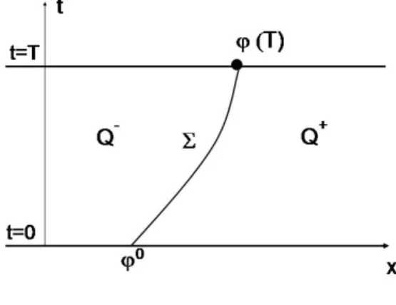
(H) Assume that u(x, t) is a weak entropy solution of (1.1) with a discontinuity along a regular curve Σ = {(t, ϕ(t)), t∈[0, T +τ]}, for some τ >0, which is uniformly Lipschitz continuous outside Σ. In particular, it satisfies the Rankine-Hugoniot condition on Σ
ϕ0(t)[u]ϕ(t) = [f(u)]ϕ(t), 0≤t≤T +τ. (4.17)
Here we have used the notation [v]x0 = v(x
+
0)−v(x
−
0) for the jump at x0 of any
piecewise continuous function v with a discontinuity at x=x0.
small perturbations of the flux functionf in (1.1) will provide solutions which still satisfy hypothesis (H), with possibly different values of τ > 0.
Note that Σ dividesR×(0, T) in two parts: Q− andQ+, the subdomains ofR×(0, T) to the left and to the right of Σ respectively.
Figure 1: Subdomains Q− and Q+.
As we will see, in the presence of shocks, for correctly dealing with optimal control and design problems, the state of the system has to be viewed as being a pair (u, ϕ) combining the solution of (1.1) and the shock location ϕ. This is relevant in the analysis of sensitivity of functions below and when applying descent algorithms.
Then the pair (u, ϕ) satisfies the system
∂tu+∂x(f(u)) = 0, in Q−∪Q+,
ϕ0(t)[u]ϕ(t) = [f(u)]ϕ(t), t∈(0, T),
ϕ(0) =ϕ0,
u(x,0) = u0(x), in {x < ϕ0} ∪ {x > ϕ0}.
(4.18)
We now analyze the sensitivity of (u, ϕ) with respect to perturbations of the fluxf. To be precise, we adopt the functional framework based on the generalized tangent vectors introduced in [9].
Definition 4.1 ([9]) Let v : R → R be a piecewise Lipschitz continuous function with a single discontinuity at y ∈ R. We define the set Γ(v,y) as the family of all continuous
paths γ : [0, ε0]→L1(R)×R with
1. γ(0) = (v, y) and ε0 >0 possibly depending on γ.
2. For any ε ∈ [0, ε0], γ(ε) = (vε, yε) where the functions vε are piecewise Lipschitz
constant L independent ofε ∈[0, ε0] such that
|vε(x)−vε(x0)| ≤L|x−x0|,
whenever yε ∈/ [x, x0].
The paths γ(ε) = (vε, yε)∈Γ(v,y) will be referred as regular variations of (v, y).
Furthermore, we define the set T(v,y) of generalized tangent vectors of (v, y) as the
space of (δv, δy)∈L1×R for which the path γ(δv,δy) given by γ(δv,δy)(ε) = (vε, yε) with
vε =
v +εδv+ [v]y χ[y+εδy,y] if δy <0,
v+εδv−[v]y χ[y,y+εδy] if δy >0,
yε=y+εδy, (4.19)
satisfies γ(δv,δy) ∈Γ(v,y).
Finally, we define the equivalence relation ∼ defined on Γ(v,y) by
γ ∼γ0 if and only if lim
ε→0
kvε−vε0kL1
ε = 0,
and we say that a path γ ∈Γ(v,y) generates the generalized tangent vector (δv, δy)∈T(v,y)
if γ is equivalent to γ(δv,δy) as in (4.19).
Remark 4.5 The path γ(δv,δy) ∈ Γ(v,y) in (4.19) represents, at first order, the variation
of a function v by adding a perturbation function εδv and by shifting the discontinuity by εδy.
Note that, for a given pair(v, y)(vbeing a piecewise Lipschitz continuous function with a single discontinuity at y∈R) the associated generalized tangent vectors (δv, δy)∈T(v,y)
are those pairs for which δv is Lipschitz continuous with a single discontinuity at x=y.
The main result in this section is the following:
Theorem 4.2 Let f ∈ C2(R) and (u, ϕ) be a solution of (4.18) satisfying hypothesis (H) in (4.17). Consider a variation δf ∈ C2(
R) for f and let fε = f +εδf ∈ C2(R)
be a new flux obtained by an increment of f in the direction δf. Assume that (uε, ϕε)
is the unique entropy solution of (4.18) with flux fε. Then, for all t ∈ [0, T] the path
(uε(·, t), ϕε(t)) is a regular variation for (u(·, t), ϕ(t)) (in the sense of Definition 4.1)
generating a tangent vector (δu(·, t), δϕ(t)) ∈L1 ×
R, i.e. (uε(·, t), ϕε(t)) ∈Γ(δu(·,t),δϕ(t)).
Moreover, (δu, δϕ)∈C([0, T]; (L1(R)×R)) is the unique solution of the system
∂tδu+∂x(f0(u)δu) =−∂x(δf(u)), in Q−∪Q+,
δϕ0(t)[u]ϕ(t)+δϕ(t) ϕ0(t)[ux]ϕ(t)−[uxf0(u)]ϕ(t)
+ϕ0(t)[δu]ϕ(t)−[f0(u)δu]ϕ(t)−[δf(u)]ϕ(t)= 0, in (0, T),
δu(x,0) = 0, in {x < ϕ0} ∪ {x > ϕ0},
δϕ(0) = 0.
We prove this technical result in an Appendix at the end of the paper.
Remark 4.6 The linearized system (4.20) has a unique solution which can be computed in two steps. The method of characteristics determinesδu inQ−∪Q+, i.e. outsideΣ, from
the initial data δu0 (note that system (4.20) has the same characteristics as (4.18)). We also have the value of uandux to both sides of the shock Σand this allows determining the
coefficients of the ODE that δϕsatisfies. Then, we solve the ordinary differential equation to obtain δϕ.
Remark 4.7 Due to the finite speed of propagation for (1.1) the result in Theorem 4.2 can be stated locally, i.e. in a neighborhood of the shock Σ. Thus, Theorem 4.2 can be easily generalized for solutions having a finite number of noninteracting shocks.
Remark 4.8 The equation forδϕin (4.20) is formally obtained by linearizing the Rankine-Hugoniot condition [u]ϕ0(t) = [f(u)] with the formula δ[u] = [δu] + [ux]δϕ.
We finish this section with the following result which characterize the solutions of (4.20).
Theorem 4.3 Let f ∈C2(R) and (u, ϕ) be a solution of (4.18) satisfying hypothesis (H) in (4.17). The solution (δu, δϕ)∈C([0, T]; (L1(
R)×R)) of the system (4.20) is given by,
δu(x, t) =−t∂x(δf(u(x, t))), in Q−∪Q+, (4.21)
δϕ(t) =t[δf(u(·, t))]ϕ(t)
[u(·, t)]ϕ(t)
, for all t∈[0, T]. (4.22)
Proof Formula (4.21) holds when u is smooth, as we stated in (4.13). The result for
u Lipschitz is easily obtained by a density argument.
We now prove formula (4.22). Without loss of generality, we focus on the caset=T. For simplicity we divide this part of the proof in two steps. First we show that
T[δf(u(·, T))]ϕ(T) =
Z
Σ
([δu],[f0(u)δu+δf(u)])·ndΣ, (4.23)
and then,
Z
Σ
([δu],[f0(u)δu+δf(u)])·n dΣ =δϕ(T)[u(·, T)]ϕ(T). (4.24)
At this point we have to introduce some notation. Let
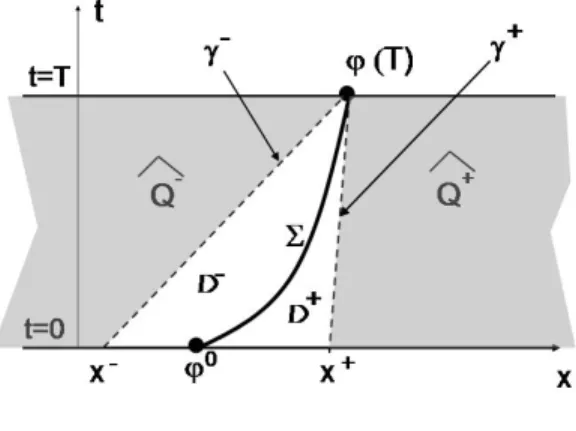
and consider the following subsets (see Figure 2),
ˆ
Q− = {(x, t)∈R×(0, T) such that x < ϕ(T)−f0(u(ϕ(T)−, T)(T −t)},
ˆ
Q+ = {(x, t)∈R×(0, T) such that x > ϕ(T)−f0(u(ϕ(T)+, T)(T −t)}, (4.26)
D− =Q−\Qˆ−, D+ =Q+\Qˆ−
. (4.27)
Note that, in ˆQ−∪Qˆ+ the characteristics do not meet the shock at any time t∈[0, T].
Figure 2: Subdomains ˆQ− and ˆQ+
In order to prove (4.23) we write the first equation in (4.20) as,
divt,x(δu, f0(u)δu+δf(u)) = 0, inQ−∪Q+. (4.28)
Thus, integrating this equation over the triangle D− = Q−\Qˆ−, using the divergence theorem and the fact that δu(x,0) =δu0(x) = 0 for all x∈
R, we obtain
0 =
Z
∂D−
(δu, f0(u)δu+δf(u))·ndσ=
Z
Σ
(δu−, f0(u−)δu−+δf(u−))·ndΣ
+
Z
γ−
(δu, f0(u)δu+δf(u))·ndσ, (4.29)
wherendenotes the normal exterior vector to the boundary ofD−and, for any continuous function v, defined in x∈Q−, we have noted
v−(x) = lim
The curve γ− in (4.29) is the characteristic line joining (t, x) = (0, x−) with (t, x) = (T, ϕ(T)). A parametrization of this line is given by
γ−:
(t, γ−(t))∈(0, T)×R such that γ−(t) =x−+tf0(u(x−,0)), and t∈(0, T) .
(4.30) With this parametrization the last integral in the right hand side of (4.29) can be written as
Z
γ−
(δu, f0(u)δu+δf(u))·n dσ=
Z T
0
δf(u(γ−(t), t))dt=T δf(u(ϕ(T)−, T)), (4.31)
where the last identity comes from the fact thatu is constant alongγ−, i.e. u(γ−(t), t) =
u(ϕ(T)−, T) for all t ∈[0, T].
Thus, taking into account (4.31), the identity (4.29) reads,
0 =
Z
Σ
(δu−, f0(u−)δu−+δf(u−))·ndΣ +T δf(u(ϕ(T)−, T)). (4.32)
Of course we obtain a similar formula if we integrate (4.28) this time over D+=Q+\Qˆ+,
0 = −
Z
Σ
(δu+, f0(u+)δu++δf(u+))·ndΣ−T δf(u(ϕ(T)+, T)), (4.33)
The sign in (4.33) is changed with respect to (4.32) since we maintain the same choice for the normal vector.
Combining the identities (4.32) and (4.33) we easily obtain (4.23).
Finally, we prove that (4.24) also holds true. We consider the following parametrization of Σ,
Σ ={(x, t)∈R×(0, T), such thatx=ϕ(t), with t∈(0, T)}. (4.34) The cartesian components of the normal vector to Σ at the point (x, t) = (ϕ(t), t) are given by
nt=
−ϕ0(t)
p
1 + (ϕ0(t))2, nx =
1
p
This, together with the second equation in system (4.20), give
[δu]Σnt+ [f0(u)δu+δf(u)]Σnx
= −ϕ
0(t)[δu(·, t)]
ϕ(t)+ [f0(u(·, t))δu(·, t) +δf(u(·, t))]ϕ(t)
p
1 + (ϕ0(t))2
= δϕ
0(t)[u(·, t)]
ϕ(t)+δϕ(t) ϕ0(t)[∂xu(·, t)]ϕ(t)−[∂x(f(u))(·, t)]ϕ(t)
p
1 + (ϕ0(t))2
= δϕ
0(t)[u(·, t)]
ϕ(t)+δϕ(t) ϕ0(t)[∂xu(·, t)]ϕ(t)+ [∂tu(·, t)]ϕ(t)
p
1 + (ϕ0(t))2
= p 1
1 + (ϕ0(t))2
d
dt δϕ(t)[u(·, t)]ϕ(t)
. (4.35)
Thus, integrating on Σ,
Z
Σ
([δu]Σnt+ [f0(u)δu+δf(u)]Σnx) dΣ =
Z T
0
d
dt δϕ(t)[u(·, t)]ϕ(t)
dt
=δϕ(T)[u(·, T)]ϕ(T)−δϕ(0)[u(·,0)]ϕ(0) =δϕ(T)[u(·, t)]ϕ(T),
where the last identity is due to the initial condition δϕ(0) = 0 in (4.20). This concludes the proof of (4.24).
4.3
Sensitivity of
J
in the presence of shocks
In this section we study the sensitivity of the functional J. This requires to study the sensitivity of the solutions uof the conservation law with respect to variations associated with the generalized tangent vectors defined in the previous section.
Theorem 4.4 Assume that f ∈ C2(
R) is a nonlinearity for which the weak entropy
solution u of (1.1) satisfies the hypothesis (H). Then, for any δf ∈C2(
R), the following
holds,
δJ = lim
ε→0+
J(f+εδf)−J(f)
ε
= −T
Z
{x<ϕ(T)}∪{x>ϕ(T)}
∂x(δf(u))(x, T) (u(x, T)−ud(x))dx
−T η
[u(·, T)]ϕ(T) [δf(u(·, T))]ϕ(T), (4.36)
where
η= 1 2
(u(·, T)−ud(ϕ(T)))2
if ud is continuous at x=ϕ(T) and,
η=
( 1
2
(u(·, T)−ud(ϕ(T)+))2
ϕ(T), if δϕ(T)>0, 1
2
(u(·, T)−ud(ϕ(T)−))2
ϕ(T), if δϕ(T)<0,
(4.38)
if ud has a jump discontinuity at x=ϕ(T).
Remark 4.9 Note that, when ud is discontinuous at x =ϕ(T), the value of η in (4.38)
depends on the sign of δϕ(T). This means that the expression of δJ in (4.36) is not necessarily the same if we take the limit as ε →0for negative values of ε. The functional J in this case is not Gateaux differentiable, in general.
Formula (4.36) coincides with (4.3) in the absence of shocks or when[δf(u(·, T))]ϕ(T) =
0. In this case the Gateaux derivative of J exists and it is as if no shocks were present. We prove later that, in fact, if this condition is satisfied, then the variation δf, to first order, does not move the shock position.
We briefly comment the above result before giving the proof. Formula (4.36) provides easily a descent direction forJ when looking for a fluxf in the finite dimensional subspace
UM
ad, defined in (2.6). In this case the derivative of the functional J at α in the tangent
direction δα= (δα1, ..., δαM)∈RM is given by
δJ(α)(δα) = −
M
X
m=1
δαm
T
Z
R
∂x(fm(u))(x, T) (u(x, T)−ud(x))dx
− ηm
[u(·, T)]ϕ(T) T [fm(u(·, T))]ϕ(T)
!
. (4.39)
where ηm is the value of η in (4.38) when δf =fm.
Thus, the steepest descent direction forJ atα is given by
δαm = T
Z
R
∂x(fm(u))(x, T) (u(x, T)−ud(x))dx
− ηm
[u(·, T)]ϕ(T) T [fm(u(·, T))]ϕ(T), for all m∈1, ..., M. (4.40)
Note however that this expression is not very useful in practice since it does not avoid to compute the linearized system (4.20) for eachfmwithm= 1, ..., M, in order to compute
ηm, since the knowledge of the sign ofδϕ(T) is required. This is due to the lack of Gateaux
Proof (of Theorem 4.4). We first prove the following,
δJ = lim
ε→0+
J(f+εδf)−J(f)
ε
=
Z
{x<ϕ(T)}∪{x>ϕ(T)}
(u(x, T)−ud(x))δu(x, T)dx−ηδϕ(T), (4.41)
where the pair (δu, δϕ) is a generalized tangent vector of (u(·, T), ϕ(T)) which solves the linearized problem (4.20) and η is defined in (4.37)-(4.38).
Let us obtain (4.41) in the particular case whereud is discontinuous at x=ϕ(T) and
δϕ(T) >0, the other cases being similar. Let fε = f +εδf and (uε, ϕε) be the solution
of (4.18) associated to the flux fε. From Theorem 4.2, (uε, ϕε) is a path for a generalized
tangent vector (δu, δϕ) satisfying (4.20). Thus, (uε, ϕε) is equivalent to a path of the form
(4.19) and we have,
1
ε(J(fε)−J(f)) =
1 2ε
Z
R
(uε(x, T)−ud(x))2dx−
Z
R
(u(x, T)−ud(x))2dx
=
Z
{x<ϕ(T)}∪{x>ϕ(T)+εδϕ(T)}
(u(x, T)−ud(x))δu(x, T)dx
+ 1 2ε
Z ϕ(T)+εδϕ(T)
ϕ(T)
u(x, T)−[u]ϕ(T)−ud(x)
2
dx
− 1
2ε
Z ϕ(T)+εδϕ(T)
ϕ(T)
u(x, T)−ud(x)2dx+O(ε)
=
Z
{x<ϕ(T)}∪{x>ϕ(T)+εδϕ(T)}
(u(x, T)−ud(x))δu(x, T)dx
+δϕ(T)
2 u(ϕ(T) −
, T)−ud(ϕ(T)+)2
−δϕ(T)
2 u(ϕ(T)
+, T)−ud(ϕ(T)+)2
+O(ε)
=
Z
{x<ϕ(T)}∪{x>ϕ(T)+εδϕ(T)}
(u(x, T)−ud(x))δu(x, T)dx
−δϕ(T)[1
2 u(x, T)−u
d
(ϕ(T)+)2]ϕ(T)+O(ε).
We obtain (4.41) by passing to the limit as ε→0.
5
Alternating descent directions
In this section we introduce a suitable decomposition of the vector space of tangent vectors associated to a flux functionf. As we will see this decomposition allows to obtain simplified formulas for the derivative of J in particular situations. For example, we are interested in those variations δf for which, at first order, the shock does not move at
t =T.
Theorem 5.1 Assume that f is a nonlinearity for which the weak entropy solution u of (1.1) satisfies the hypothesis (H) and, in particular, the Rankine-Hugoniot condition (4.17). Letδf ∈C2(R)be a variation of the non-linearityf and(δu, δϕ)the corresponding solution of the linearized system (4.20). Then, δϕ(T) = 0 if and only if
[δf(u(·, T))]ϕ(T) = 0. (5.1)
Moreover, if condition (5.1) holds, the generalized Gateaux derivative of J at f in the direction δf can be written as
δJ =−T
Z
R
∂x(δf(u))(x, T)(u(x, T)−ud(x))dx. (5.2)
Proof. The characterization (5.1) follows from the identity (4.22). On the other hand, formula (5.2) is a particular case of identity (4.36).
Remark 5.1 Formula (5.2) provides a simplified expression for the generalized Gateaux derivative of J when considering variations δf that do not move the shock position at t = T, at first order, i.e. those for which δϕ(T) = 0. These directions are characterized by formula (5.1).
In practice we assume that the fluxes f are taken in the finite dimensional space UM ad,
defined in (2.6). The set UM
ad can be parametrized by α = (α1, ..., αM) ∈ RM. The
condition (5.1) reads
M
X
m=1
αm[δfm(u(·, T))]ϕ(T) = 0, (5.3)
which defines an hyperplane in RM, corresponding to the set of vectors (α1, ..., αM)∈RM
orthogonal to
([δf1(u(·, T))]ϕ(T), ...,[δfM(u(·, T))]ϕ(T))∈RM. (5.4)
The results in Theorem 5.1 suggest the following decomposition of the tangent space
Tα =RM constituted by the variations δα∈RM of a vector α∈RM:
Tα =Tα1 ⊕T
2
where T1
α is the subset constituted by the vectors (δα1, ..., δαM) satisfying (5.3); and the
one-dimensional subspace Tα2, generated by (5.4).
According to (4.39) and (5.2), the derivative of the functional J at α in the tangent direction δα= (δα1, ..., δαM)∈ Tα1 is as in (4.4) and the steepest descent direction for J
at α, when restricted to T1
α, is then given by (4.5).
Roughly speaking, we have obtained a steepest descent direction for J among the variations which do not move the shock position at t=T, i.e. δϕ(T) = 0.
On the other hand, T2
α defines a second class of variations which allows to move the
discontinuity of u(x, T).
Note that, contrarily to [11] we do not consider the class of variations that, moving the shock, do not deform the solutiom away from it since this class is generically empty on the present context in which the nonlinearity is perturbed by a finite number of parameters. We now define a strategy to obtain descent directions forJ atf. To illustrate this we consider the simplest case, i.e.
ud are Lipschitz continuous with a discontinuity atx=xd. (5.6)
As the solution u has a shock discontinuity at the final time t = T, located at some point x=ϕ(T), there are two possibilities, depending on the value ofϕ(T):
1. ϕ(T) 6= xd. Then, we perturb f with variations in T2
α until we have xd = ϕ(T).
This is in fact a one-dimensional optimization problem that we can solve easily.
2. We already have xd = ϕ(T) and then we consider descent directions δf ∈ Tf1. To first order, these directions will not move the value of ϕat t=T, but will allow to etter fit the value of the solution to both sides of the shock.
In practice, the deformations of the second step will slightly move the position of the shock because the condition δϕ(T) = 0 that characterizes variations in the subspace T1
f,
only affects the position of the discontinuity at first order. Thus, one has to iterate this procedure to assure a simultaneous better placement of the shock and a better fitting of the value of the solution away from it.
In the next section we explain how to implement a descent algorithm following these ideas that, of course, can also be used in the case where the number of shocks of u0 and
ud is not necessarily one, or the same.
6
Numerical approximation of the descent directions
We have computed the gradient of the continuous functional J in several cases (usmooth and having shock discontinuities) but, in practice, one has to look for descent directions for the discrete functional J∆. In this section we discuss the various possibilities for
searching them depending on the approach chosen (continuous versus discrete) and the degree of sophistication adopted.
We consider the following possibilities:
• The discrete approach: differentiable schemes.
• The discrete approach: non-differentiable schemes.
• The continuous approach.
• The continuous alternating descent method.
The last one is the new method we propose in this article by adapting the one intro-duced in [11] in the context of inverse design in which the control is the initial datum.
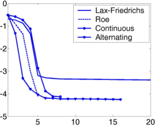
In the following Section we present some numerical experiments that allow us to easily compare the efficiency of each method. As we shall see, the alternating descent method we propose, alternating the variations of the flux to sometimes move the shock and some others correct the profile to both sides of it, is superior in several ways. It avoids the drawbacks of the other methods related either to the inefficiency of the differentiable methods to capture shocks or the difficulty of dealing with non-differentiable schemes and the uncertainty of using “pseudo-linearizations”. As a consequence of this, the method we propose is much more robust and makes the functional J decrease in a much more efficient way in a significantly smaller number of iterations.
on the discretization of the continuous gradient while the fourth subsection is devoted to the new method introduced in this work in which we consider a suitable decomposition of the generalized tangent vectors.
We do not address here the convergence of descent algorithms when using the approx-imations of the gradients described above. In the present case, and taking into account that when dealing with the discrete functional J∆ the number of control parameters is
finite, one could prove convergence by using LaSalle’s invariance principle and the cost functional as Lyapunov functional, at least in the case of the discrete approach.
6.1
The discrete approach: Differentiable numerical schemes
Computing the gradient of the discrete functional J∆ requires calculating one derivative
of J∆ with respect to each node of the mesh. This can be done in a cheaper way using
the adjoint state. We illustrate it on the Lax-Friedrichs numerical scheme. Note that this scheme satisfies the hypothesis of Theorem 3.1 and therefore the numerical minimizers are good approximations of minimizers of the continuous problem. However, as the discrete functionals J∆ are not necessarily convex the gradient methods could possibly provide
sequences that do not converge to a global minimizer of J∆. But this drawback and
difficulty appears in most applications of descent methods in optimal design and control problems. As we will see, in the present context, the approximations obtained by gradient methods are satisfactory, although convergence is slow due to unnecessary oscillations that the descent method introduces.
Computing the gradient of J∆, rigourously speaking, requires the numerical scheme
(3.3) under consideration to be differentiable and, often, this is not the case. To be more precise, for the scalar equation (1.1) we can choose efficient methods which are differentiable (as the Lax-Friedrichs one) but this is not the situation for general systems of conservation laws in higher dimensions, as Euler equations. For such complex systems the efficient methods, as Godunov, Roe, etc., are not differentiable (see, for example [22] or [28]) thus making the approach in this section useless.
We observe that when the 3-point conservative numerical approximation scheme (3.3) used to approximate the scalar equation (1.1) has a differentiable numerical flux function
g, then the linearization is easy to compute. We obtain
δunj+1 =δun j −λ
δgn
j+1/2+∂1g
n j+1/2δu
n
j +∂2gnj+1/2δunj+1
−δgn
j−1/2−∂1g
n j−1/2δu
n
j−1−∂2gjn−1/2δu
n j
, j ∈Z, n = 0, ..., N.
(6.1)
Here, δgn
j+1/2 =δg(u
n
j, unj+1) where δg represents the Gateaux derivative of the numerical
of (4.10).
On the other hand, for any variationδf ∈ Uad off, the Gateaux derivative of the cost
functional defined in (3.2) is given by
δJ∆= ∆x
X
j∈Z
(uNj +1−udj)δuNj +1, (6.2)
which is the discrete version of (4.12).
It is important to observe that here we cannot solve system (6.1) to obtain the discrete version of (4.13), as in the continuous case, since it is based on a characteristic construction which is difficult to translate at the discrete level. Thus, unlike in the continuous case, we must introduce a discrete adjoint system to obtain a simplified expression of the Gateaux derivative (6.2).
The discrete adjoint system for any differentiable flux function g is,
(
pn
j =pnj+1+λ
∂1gnj+1/2(p
n+1
j+1 −p
n+1
j ) +∂2gjn−1/2(p
n+1
j −p
n+1
j−1)
, pNj +1 =uNj +1−ud
j, j ∈Z, n = 0, ..., N.
(6.3)
In fact, when multiplying the equations in (6.1) by pnj+1 and adding in j ∈ Z and n = 0, ..., N, the following identity is easily obtained,
∆xX
j∈Z
(uNj +1−udj)δuNj +1 =−∆xλ
N
X
n=0
X
j∈Z
(δgnj+1/2−δgjn−1/2)p
n+1
j . (6.4)
This is the discrete version of the identity
Z
R
(u(x, T)−ud(x))δu(x, T)dx=−
Z T
0
Z
R
∂x(f0(u(x, t)))p(x, t)dx dt,
which holds in the continuous case, and it allows us to simplify the derivative of the discrete cost functional. Note also that (6.3) is also a particular discretization of the adjoint system
−∂tp−f0(u)∂xp= 0, x∈R, t∈(0, T),
p(x, T) =u(x, T)−ud(x), x∈R.
In view of (6.3) and (6.4), for any variation δf ∈ Uad of f, the Gateaux derivative of
the cost functional defined in (3.2) is given by
δJ∆= ∆x
X
j∈Z
(uNj +1−udj)δuNj +1 =−∆xλ
N
X
n=0
X
j∈Z
which is the discrete version of
δJ =−
Z T
0
Z
R
∂x(δf(u(x, t)))p(x, t)dx dt.
Formula (6.5) allows to obtain easily the steepest descent direction for J∆. In fact,
given f ∈ UM
ad with f =
PM
m=1αmfm for some coefficientsαm ∈R, and
δf =
M
X
m=1
δαmfm,
making explicit the dependence of the numerical fluxgonf by writingg(u, v) = g(u, v;f), we have
δgjn+1/2 =δg(unj, unj+1;f) =∂fg(unj, u n
j+1;f)δf =
M
X
m=1
∂fg(unj, u n
j+1;f)fmδαm.
When substituting in (6.5), we obtain
δJ∆ =−∆xλ
N
X
n=0
X
j∈Z
M
X
m=1
(∂fg(unj, u n
j+1;f)fm−∂fg(unj−1, u
n
j;f)fm)δαm pnj+1, (6.6)
and a descent direction for J∆ atf
∆ is given by
δαm = ∆xλ N
X
n=0
X
j∈Z
(∂fg(unj, u n
j+1;f)fm−∂fg(unj−1, u
n
j;f)fm)pnj+1. (6.7)
Remark 6.1 At this point it is interesting to compare formulas (6.6) and (6.7) with their corresponding expressions at the continuous level, i.e. formulas (4.4) and (4.5) respectively. The discrete formulas are obtained by projecting formula (6.5) into the finite dimensional subspace UM
ad, while the continuous ones come from the projection of the
simplified expression (4.4). As we have said before, we do not know how to obtain a discrete version of (4.4) from (6.5).
Remark 6.2 We do not address here the problem of the convergence of these adjoint states towards the solutions of the continuous adjoint system. Of course, this is an easy matter when u is smooth but is far from being trivial when u has shock discontinuities. Whether or not these discrete adjoint systems, as ∆ → 0, allow reconstructing the com-plete adjoint system, with the inner Dirichlet condition along the shock, constitutes an interesting problem for future research. We refer to [23] for preliminary work on this direction.
6.2
The continuous approach
This method is based on the result stated in Theorem 4.4 indicating that the sensitivity of the functional is obtained by formula (4.3). In particular, when considering the finite dimensional subspace UM
ad, the steepest descent direction is given by (4.4). A tentative
descent direction for the discrete functional is then obtained by a numerical approximation of (4.4). One possible choice is to take, for each m∈1, ..., M,
δαm = T
X
j∈Z
(fm(uNj+1+1)−fm(uNj +1))
uNj +1+uNj+1+1
2 −
udj +udj+1
2
!
, (6.8)
where un
j is obtained from a suitable conservative numerical scheme regardless of its
differentiability. This formula is obviously consistent with the components of the steepest descent direction in (4.5), if no shocks are present.
6.3
The alternating descent method
Here we propose a new method inspired by the results in Theorem 5.1 and the discussion thereafter. We shall refer to this new method as the alternating descent method, that was first introduced in [11] in the context of an optimal control problem for the Burgers equation where the control variable is the initial datum.
To fix ideas we assume that we look forf in the finite dimensional subspaceUM ad. We
also assume that both the target ud and the initial datum u0 are Lipschitz continuous
functions having one single shock discontinuity. But these ideas can be applied in a much more general context in which the number of shocks is larger and even do not necessarily coincide.
solutionu of (1.1) at timet =T, regardless of its value to both sides of the discontinuity. Once this is done we perturb the resulting f so that the position of the discontinuity is kept fixed and alter the value of u(x, T) to both sides of it. This is done by decomposing the set of variations associated to f into the two subsets introduced in (5.5), considering alternatively variations δα ∈Tα1 and δα ∈Tα2 as descent directions.
For a given initialization off, in each step of the descent iteration process we proceed in the following three sub-steps:
1. Determine the subspacesT1
α and Tα2 by computing the vector (5.4). Note that Tα2 is
in fact a one-dimensional subspace.
2. We consider the vector (5.4) that generates T2
α, and choose the optimal step, so to
minimize the functional in that direction of variation of the nonlinearity f. This involves a one-dimensional optimization problem that we can solve with a classical method (bisection, Armijo’s rule, etc.). In this way we obtain the best location of the discontinuity on that step.
3. We then use the descent direction δα ∈ Tα1 to modify the value of the solution at time t =T to both sides of the discontinuity. Here, we can again estimate the step size by solving a one-dimensional optimization problem or simply take a constant step size.
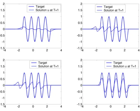
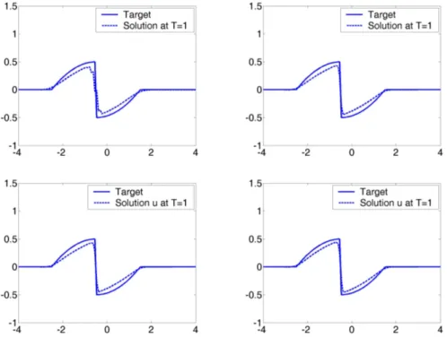
7
Numerical experiments
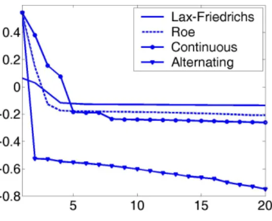
In this section we present some numerical experiments which illustrate the results obtained in an optimization model problem with each one of the numerical methods described in this paper.
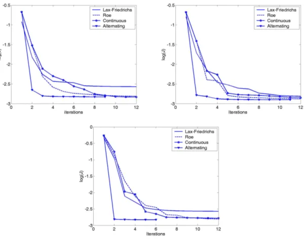
The following numerical methods are considered:
1. The discrete approach with the Lax-Friedrichs scheme. The optimization procedure is based on the steepest descent method and the descent directions are computed using the adjoint approach.
2. The discrete approach with the Roe scheme. It has the numerical flux,
gR(u, v) = 1
2(f(u) +f(v)− |A(u, v)|(v−u)),
where the matrix A(u, v) is a Roe linearizationwhich is an approximation of f0. In the scalar case under consideration A(u, v) is a function given by,
A(u, v) =
f(u)−f(v)
u−v , if u6=v,
The optimization procedure is again based on the steepest descent method and the descent directions are computed using the adjoint approach. We recall that unlike the Lax-Friedrichs scheme this one is not differentiable and the adjoint system is obtained formally (see [19], [11]).
3. The continuous approach with the Roe scheme. We use the method described in subsection 6.2. In this case, as we discretize the continuous adjoint system, the use of a differentiable or a non-differentiable scheme is not relevant to approximate the direct problem. However, in practice, a numerical scheme based on a pseudo-linearization of the scheme used for the direct problem is usually more efficient. This pseudo-linearization is usually obtained by considering a particular choice of the subdifferential in the regions where the scheme is not differentiable.
4. The continuous approach with the Roe scheme using the generalized tangent vectors decomposition and the alternating descent method described in subsection 6.3.
We have chosen as computational domain the interval (−4,4) and we have taken as boundary condition in (1.1), at each time step t = tn, the value of the initial data at
the boundary. This can be justified if we assume that both the initial and final data u0,
ud take the same constant value ¯u in a sufficiently large neighborhood of the boundary
x = ±4, and the value of f0(¯u) does not become very large in the optimization process, due to the finite speed of propagation. A similar procedure is applied for the adjoint equation.
In our experiments we assume that the flux f is a polynomial. The relevant part of the flux function is its derivative since it determines the slope of the characteristic lines. Thus, we take f0 of the form
f0(u) = α1P1(u) +α2P2(u) +...+α6P6(u),
where αj are some real coefficients and Pj(u) are the Legendre polynomials, orthonormal
with respect to the L2(a, b)-norm. The interval [a, b] is chosen in such a way that it
contains the range of u0, and therefore the range of the solutions u under consideration.
To be more precise, we take [a, b] = [0,1] and then
P1(u) = 1,
P2(u) =
√
12(u−1/2), P3(u) =
√
80(3/2u2−3/2u+ 1/4),
P4(u) =
√
448(5/2u3−15/4u2+ 3/2u−1/8), P5(u) =
√
2304(35/8u4−35/4u3+ 45/8u2−5/4u+ 1/16), P6(u) =
√
11264(63/8u5 −315/16u4+ 35/2u3−105/16u2+ 15/16u−1/32).