A numerical study of the development of convection on
21 July 2001 over Cuba
D. R. POZO, J. C. MARÍN
Centro de Ciencias de la Atmósfera, Universidad Nacional Autónoma de México, Circuito Exterior, Ciudad Universitaria, México, D. F. 04510 México
Corresponding author: D. R. Pozo; e-mail: [email protected]
I. BORRAJERO, D. MARTÍNEZ and A. BEZANILLA
Instituto de Meteorología, Apdo. 17032, La Habana 17, Cuba
Received October 8, 2004; accepted March 17, 2006
RESUMEN
ABSTRACT
On 21 July 2001 several severe storms developed over the eastern region of Cuba in the afternoon hours and hail was observed. A numerical simulation was performed to study the structure and evolution of convection on that day with the aid of the 1800 UTC sounding. Furthermore, three more simulations were performed to study the effect of the vertical wind profile on the severity of the simulated storms. The Advanced Regional Prediction System model (ARPS) was used for this numerical study. An initial storm that later split into two new storms that moved to the right and to the left of the mean wind was simulated. The right-moving storm (RS) developed more than the left-moving one (LS). Hail was observed in most of the simulation time but the largest amount of hail reached the surface after the splitting in the RS. Two mechanisms were responsible for the inhibition of the LS. First, a vertical pressure gradient that acted against the main updraft development. Second, the entrainment of drier and colder air in the LS’s updraft at midlevels that came directly from the downdraft region. The wind shear above 10 km was favorable for a larger hail production, intensity and maximum values at the surface and a larger precipitation area. When the wind shear below 7 km was removed, the total volume of precipitation, the intensity of precipitation, maximum horizontal wind and maximum updraft were the largest compared to the other simulations. The LS was not inhibited in this case and both storms reached the same strength. The mechanisms that inhibited the development of the LS were not present in this simulation.
Keywords: Storm splitting, numerical simulation, mesoscale meteorology.
1. Introduction
Many numerical studies have investigated the combined or individual influence of the vertical wind shear and the bouyancy on the structure and development of convective storms (Klemp and Wilhelmson, 1978a, b; Wilhelmson and Klemp, 1978; Schlesinger, 1980; Fovell and Ogura, 1989; McCaul and Weisman, 2001) and resulted in a better understanding on this matter.
In the afternoon hours of 21 July 2001, several severe storms developed over the eastern region of Cuba, where hail was observed. Hailstorms are severe and uncommon in Cuba, and deserve investigation. In order to study the structure and evolution of the convection that developed that day, a numerical simulation was performed. One of the goals is to explore whether a hailstorm could be simulated with an initially homogeneous environment as condition. The 1800 UTC sounding taken at the meteorological surface station of Camagüey (located in that region) was used to define the initial basic state.
Based on the wind profile of the observed sounding, a set of three more simulations was designed to study the influence of the wind profile on the severity of the simulated storms. The severity was studied in terms of the ability of the storms to produce large amount of rain, hail and strong winds. The Advanced Regional Prediction System (ARPS) was used in this study.
2. Meteorological situation of 21 July 2001
237 A numerical study of the development of convection on 21 July 2001 over Cuba
The 1800 UTC sounding from the Camagüey station (21° 25´ N, 77° 10´ W) (Fig. 1a) exhibits a deep moist layer, a well-mixed sub-cloud layer and high convective available potential temperature (CAPE), of 3351 J/kg. The low level wind is relatively weak, with variable direction from W-SW at low levels, but turning preferentially clockwise up to 10 km, at the base of a jet from the NE that extends to 16 km (Fig. 1b). The wind profile presents three different layers in the troposphere: a low level shear layer from the surface to 7 km, a higher level shear layer with wind speeds increasing with height from 7 to 14 km, and a layer with wind speed decreasing with height from 14 to 16 km.
Fig. 1. a) 1800 GMT sounding of 21 July 2001, measured at the meteorological surface station of Camagüey. b) Representation of the hodograph measured at that hour.
3. Model description and initialization
The numerical model ARPS (Version 4.5.1, in its 3-dimensional configuration), a non-hydrostatic and compressible model valid for scales ranging from a few meters to hundreds of kilometers, was
used (Xue et al., 1995). ARPS has been tested and widely used in numerical studies (Xu et al., 1996;
Fovell and Tan, 1998; Xue et al., 2001). Detailed information can be found in Xue et al. (2000, 2001,
and 2003).
A second order momentum advection was used as well as a sub-grid turbulence parameterization of order 1.5, which involves the solution of an additional forecast equation for the turbulent kinetic
energy. The microphysics parameterization scheme of Lin et al. (1983) for solid and mixed phase
processes was selected. The effects of orography, land-use and radiation were not included in order to simplify the model configuration.
A nu
TTheT
-60
-90-80-70 -50 -40 -30 -20 -10 0 10 20 30 40NE E SE S SW WNWN
2 5 0 5 0 7 5 100
Relative humidity, %
3 0
0 1 5 4 5 6 0 7 59 0 105
Wind speed, m/s
Temperature °C Wind direction
a) b)
v(m/s)
30 3 6 10 20
50 70 100
150 200 250 300 400 500 600 700 850 1000
u
u(m/s)
Pressure, hPa
1
The lateral boundary condition proposed by Klemp and Wilhelmson (1978a) was used. In this study, the initial perturbation bubble was located in the center of the domain to diminish the interaction with the lateral boundaries. For the top of the domain and the underlying surface, the rigid wall condition was assumed.
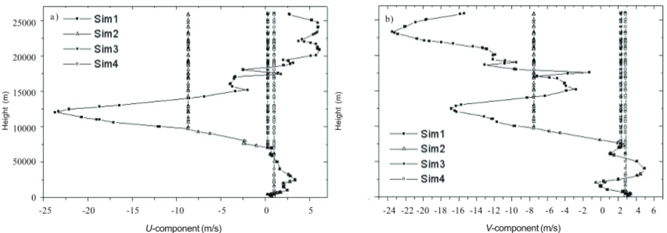
A set of four numerical experiments was conducted. The first simulation, called Sim1 hereafter, was initialized with the 1800 UTC sounding taken at Camagüey station (21° 25´ N and 77° 10´ W) and represents the simulation of the real storm. The rest of the simulations were designed by varying the wind profile in the original sounding in order to investigate the effects of the wind profile on the severity of the simulated storms.
The second simulation (Sim2) was initialized with a sounding where the wind above 10 km was made constant and equal to the wind speed at 10 km to eliminate the effects of the strong northeastern winds above that height. In the third simulation (Sim3), the wind was made constant from 7 km upward to eliminate the strong unidirectional shear associated with the large variations in wind direction and strength between 7 and 10 km in the original sounding. Note that despite the original wind shear is still unidirectional between 10 and 12 km, winds are stronger and variations in direction are smaller than at lower levels. Lastly, the fourth simulation (Sim4) was initialized with a sounding that presents constant u and v components of the wind with height (no shear). This allows us to
assess how the storm would develop without any vertical shear. The u and v components of the
wind profile for all simulations can be seen in Figure 2.
Fig. 2. Wind profiles used in the simulations: a) U-component of the wind b) V-component of the wind.
A 90 × 96 km grid was used with a horizontal resolution of 1 km. In the vertical, 40 levels with
a constant resolution of 0.5 km were chosen. The center of the domain was located at nearly 45 km past the Camagüey sounding station, at 21° 35´ N and 77° 33´ W near the place where the storms developed. The simulation was run for 3 hours, a time step of 6 s was used and output results every 60 s were saved.
a ) b)
-24 -22 -20 -18 -16 -14 -12-10 -8 -6 -4 -2 0 2 4 6
-15 -10 -5 0 5
-20 -25
V-component (m/s)
U-component (m/s) 25000
20000
15000
10000
50000
0
To initiate convection, a warm perturbation was used. This method may not be rigorous to simulate the initiation of convection but due to its simplicity it has been widely used in three-dimensional numerical simulations of thunderstorms structure (Klemp and Wilhelmson 1978a, b; Weisman and Klemp, 1984; Rotuno and Klemp 1985; McCaul and Weisman 2001) with satisfactory results. The
perturbation was centered at x = 50 km, y = 37 km from the origin of the domain and z = 1.5 km,
with radial dimensions of 10 km in the x, 30 km in the y and 1.5 km, in the z directions, and a
maximum potential temperature excess of 4 K. The potential temperature excess in the bubble diminish through space in the horizontal and vertical directions with respect to their maximum value located at its center. The parameters of the perturbation were chosen as the minimum values required to obtain a development of convection for several hours.
4. Results
4.1 Structure and physical mechanisms of the 21 July 2001 convection (Sim1)
The initial cloud formed at 660 s of simulation at the location of the initial perturbation. At that time,
the cloud water content (qc) is the only hydrometeor present, with a maximum value of 0.1 g/kg. At
900 s it reaches a maximum value of 1 g/kg. At 1380 s, the rain water content (qr) reaches 4 g/kg,
the cloud top is higher than 6 km, and the ice cloud content (qi) can be appreciated. The latent heat
released by the phase transformations accelerates the updrafts at the higher levels of the cloud reaching maximum values larger than 30 m/s. The rapid strengthening of the updraft from the middle troposphere up to the higher levels is also a consequence of the high CAPE. The hail
content (qh) is very large at this relatively early stage of the cloud life, and fall through the central
part of the updraft, having its maximum (>20 g/kg) in the lower part of the cloud. Part of qh is
located lower than the 0 °C isotherm, contributing to rain formation by melting.
The vorticity and vertical velocity fields are shown in a horizontal plane at 2 km height (Fig. 3a) at 1800 s. Two vorticity centers of opposite sign are observed within the updraft region in the cloud. They are initiated due to the tilting of horizontal vorticy, which was provided by the vertical wind shear, by the updrafts present in the initial cloud development, as has been mentioned by Schlesinger (1978), Klemp and Wilhemson (1978b), and Weisman and Klemp (1984) in numerical simulations, and Barnes (1970) with mesonetwork data analysis. The region of maximum updraft is located between the vorticity centers and a small region of minimun updraft is seen, related to the rain water that reaches the surface at this time and provide the generation of downdrafts.
After 1800 s of simulation a spliting process starts to occur, which generates two new cells that move to the right (RS) and left (LS) of the parent storm motion. Hail content values of 0.1 g/kg are observed reaching the surface at 2040 s before the complete splitting of the parent storm. At 2880 s, after the splitting has occurred, two regions of hail content are present at the surface associated with both cells and continue until 3480 s. From this time, only a region of hail content associated with the RS persists and increases in diameter, reaching a maximum value of 5 g/kg at 3960 s.
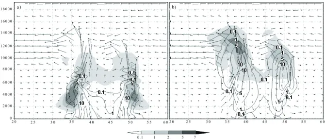
In Figure 4 a, b the new cells are observed, in a vertical plane drawn at x = 56.5 km (3000 s).
4a, a downdraft located between both cells and isolines of maximum values of qr can be seen
reaching the surface. The qc values are located on the outward sides of both cells coincident with
the main updrafts at the midlevels (4 to 6 km). The main updrafts increase in intensity at higher levels, where maximum values of qi are located, related with the large amount of latent heat released
(Fig. 4b). Furthermore, in the same figure, two maximum regions of qh associated with both cells
can also be seen. All this give evidence that the split occurred.
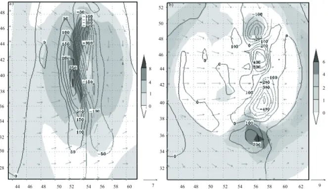
At 3000 s of simulation (Fig. 3b), four vorticity centers are shown in a horizontal plane at 2 km height. The two new centers (located to the north/south of the RS/LS) were generated by the downdraft that provides the tilting of the horizontal vorticity. The main updrafts in the RS/LS rotate cyclonically/anticyclonically and the new vorticity centers are located within the downdraft region. Despite similar patterns found in previous works (Klemp and Wilhelmson, 1978b; Schlesinger 1980; Wilhelmson and Klemp, 1981) that favor the development of supercells in the RS (with a clockwise turning hodograph), the magnitude of the vertical vorticity is much smaller in this case. It is a consecuence of the chaotic behavior of the hodograph from the surface to midlevels where a small clockwise turning tendency can be appreciated, but weak wind shear values dominate. The stronger development reached by RS in the current simulation will be further analyzed.
Fig. 3. Horizontal cross section at 2 km height. The shaded areas represent the vertical velocity and the isolines represent the vertical vorticity. a) At 1800 s. b) At 3000 s. The x-axis increases in km to the east and they-axis increases in km to the north.
50
44 46 48 52 54 56 58 60 7 46 48 50 52 54 56 58 60 62 9
6
4
2
1
0 46
44
42
40
38
32 34 36 48
8
4
0 1
52
50 b)
42
40
38
36
34
28 30 32 48
46
The pressure perturbation field in a horizontal plane at 2 km height (at 3000 s) shows that both updraft zones nearly coincide with two pressure minima, independent of the vorticity sign (Fig. 5a) (Houze, 1993). However, the RS presents larger negative values of pressure perturbation at its center enhancing the low level convergence (Davies-Jones, 1985). The negative pressure perturbation values extend through the midlevels (Fig. 5b). Above 8 km a high pressure perturbation region is located in the updraft of LS, which provides a pressure gradient acting against the LS’s upward motions. In the outward side of RS, a negative pressure perturbation region persists favoring upward motions and its larger development with respect to LS. This asymmetry in the pressure perturbation field is observed since the early stages of the storm splitting until the dissipation of LS. It is due to the presence of high wind shear values above 7 km height that increase the pressure field in the upshear cell (LS). On the other hand, an analysis of the wind structure of the system reveals other mechanism that could favor the larger development of RS. Figure 6 shows a horizontal cross section at 4 km height (3240 s). Mainly more moist air coming from the south is observed to enter the RS’s main updraft, which favors its maintenance. Nevertheless, drier air coming from the southwest (where precipitation falls from the anvil) is incorporated into the LS. This mechanism was discussed by Grass (2000) as one of the possible causes of asymmetry in the development of split storms.
At 4200 s of simulation the LS starts to decay, which is better observed at low and midlevels. However, at higher levels LS mantains its structure for some time though the area of the main updraft is smaller than that of the RS. At 4440 s, precipitation reaching the surface is observed in both cells, but hail is seen falling only from the RS, which lasts until 5160 s.
Fig. 4. Vertical cross sections passing through the plane of maximum updraft of RS (x = 56.5 km) at 3000 s. a) Cloud water (shaded areas) and rain water (isolines) mixing ratios. b) Ice water (shaded areas) and hail (isolines) mixing ratios. Vectors represent the wind field and the mixing ratios of hidrometeors are drawn in g/kg.
12000 10000 8000
2000 18000 16000 14000
6000 4000
0
7 5 2 1 0 . 1
b)
1 2 0 0 0
1 0 0 0 0
8 0 0 0
2 0 0 0 1 8 0 0 0
1 6 0 0 0
1 4 0 0 0
6 0 0 0
4 0 0 0
0
4 5 4 0 3 5 3 0 2 5
2 0 5 0 5 5
4 5 5 0 5 5 6 0 4 0
3 5 3 0 2 5
2 0 6 0
Fig. 5. Pressure perturbation (contour) and vertical velocity (shaded areas) fields at 3000 s. a) Horizontal cross section drawn at 2 km height. b) Vertical plane passing through maximum updraft value of LS at x = 56 km. The thick dashed line represents the 0.1 g/kg contour of qc.
Fig. 6. Horizontal cross section at 4 km height (3240 s of simulation). The shaded areas represent the vertical velocity, solid isolines represent the total hidrometeor content (qc + qr+qh+qs), the thick dashed isoline represents the 0.1 g/kg contour of the perturbation water vapor content (qv) and vectors represent the horizontal velocity field.
44
42
40
38
36
32 34 52
50
48
46
52
46 48 50 54 56 58 60 62
10 0 10
1 5
8000
6000
4000
2000 0 18000 16000
14000
12000 10000
3 9 4 2 4 5 4 8 5 1 5 4
3 6
3 3
3 0
5 4 5 1 4 8 4 5 4 2
3 9 5 7 6 0 6 3 2 4 2 7 3 0 3 3 3 6 3 9 4 2 4 5 4 8 5 1 5 4 5 7 3 0 0 1 5 1 0
b) a )
4.2 Sensitivity studies to the vertical wind profile
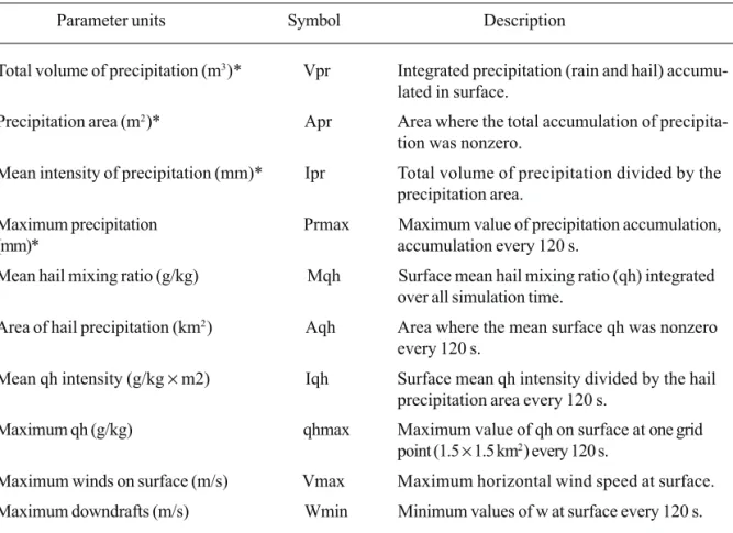
Three more simulations (Sim2, Sim3 and Sim 4) were performed in order to study the effect of the wind shear at various heights on the severity of the simulated storms. To analyze the severity, several parameters were selected related with rain, hail and surface winds, as described in Table I. All of them were calculated approximately at 250 m above the ground as a measure of the effects of storms severity on surface. Hereafter, this level will be referred to as surface.
4.3 Analysis of rain
The total volume of precipitation (Vpr) shows the same behavior in time in Sim1, Sim2 and Sim3 (Fig. 7a). In Sim 4, Vpr is 8% larger than in any other simulation starting from 5000 s. Sim1 presents the largest precipitation area (Apr) (Fig. 7b). When the shear above 10 km is removed in Sim2, Apr decreases. Apr decreases even more in Sim3 when the wind shear above 7 km is removed. This
Parameter units Symbol Description
Total volume of precipitation (m3)* Vpr Integrated precipitation (rain and hail)
accumu-lated in surface.
Precipitation area (m2)* Apr Area where the total accumulation of
precipita-tion was nonzero.
Mean intensity of precipitation (mm)* Ipr Total volume of precipitation divided by the
precipitation area.
Maximum precipitation Prmax Maximum value of precipitation accumulation,
(mm)* accumulation every 120 s.
Mean hail mixing ratio (g/kg) Mqh Surface mean hail mixing ratio (qh) integrated
over all simulation time.
Area of hail precipitation (km2) Aqh Area where the mean surface qh was nonzero
every 120 s.
Mean qh intensity (g/kg × m2) Iqh Surface mean qh intensity divided by the hail
precipitation area every 120 s.
Maximum qh (g/kg) qhmax Maximum value of qh on surface at one grid
point (1.5 × 1.5 km2) every 120 s.
Maximum winds on surface (m/s) Vmax Maximum horizontal wind speed at surface.
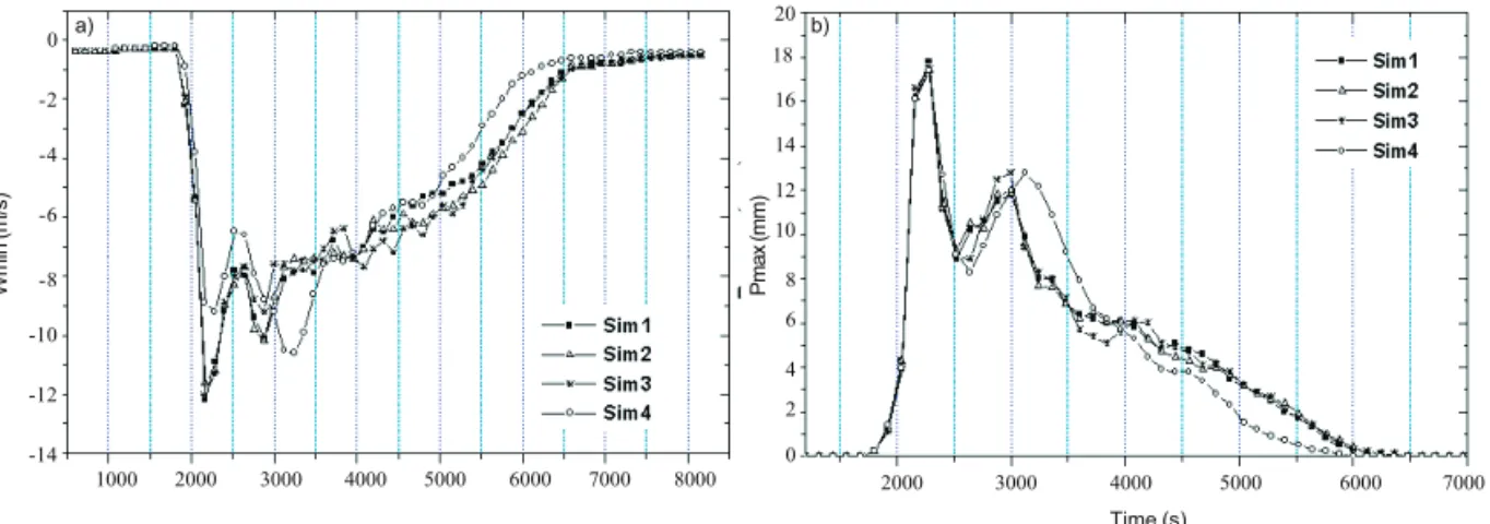
Maximum downdrafts (m/s) Wmin Minimum values of w at surface every 120 s.
Table I. Description of the parameters selected to analyze the severity of the simulated storms.
could be related to the precipitation that falls under the anvil, which is larger in Sim1 and Sim2 due to strong winds at high levels. However, when the wind shear at all levels is removed in Sim4, a larger Apr is observed in Sim 4 than in Sim3, starting from 3500 s of simulation though the difference is not so large. The reason for this could be that in Sim4 both clouds reach the same development producing more rain. Vpr is the largest in Sim4, decreasing through Sim3 and Sim2, with Sim1 being the smallest.
Fig. 7. a) Vpr (rain + hail) multiplied by 104 accumulated on surface over the horizontal domain for all
simulations. b) Apr on surface (multiplied by 106) for all simulations.
The maximum precipitation accumulation every 120 s (Prmax) includes rainwater and hail (snow is not included since it does not reach the surface). The peaks of maximum value of qh on surface every 120 s (qhmax) and Prmax are observed in figures 9b and 8b at 2160 s and the distribution of Prmax on surface (not shown) is similar in all simulations at this time. Surface plots of Prmax and qh at 3120 s (when the storm splitting has occurred) are shown in Figure 10. Some differences exist among Sim1, Sim2 and Sim 3. Sim1 and Sim 2 show a similar pattern of Prmax but qh values are present only in the northern (LS) storm of Sim1, although larger qh values are later observed in the southern (RS) storm. The Prmax area spreads in the direction where the system’s anvil is located and shows asymmetry in both simulations. Sim3 presents a smaller area of minimum Prmax values, however in LS, the area of maximun values of Prmax is larger. Furthermore, qh values are also observed.
On the other hand, Sim4 shows a symmetrical pattern of Prmax with two isolated areas of maximum values larger than 5 mm. This is related with a split process where no preferred storm is favored, which is in agreement with the removal of the low-level wind shear.
b) a)
2000 3000 4000 5000 6000 7000 8000 1000 2000 3000 4000 5000 6000 7000 8000
Time (s) Time (s)
500
400
0 100 200 300
Vpr (m
3)
×
10
4
Apr (m
2)×
10
6
400
Fig. 8. Distribution in time of a) Wmin for all simulations and b) Prmax for all simulations.
4.4 Analysis of winds
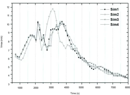
Figure 11 shows the evolution in time of maximum horizontal winds (Vmax) at surface (250 m). In general, the behavior of maximum winds at this level is similar for the first three simulations. They show a first peak associated with convergence at earlier stages of clouds development (1560 s for Sim3, 1680s for Sim1 and Sim 2 and 1800s for Sim 4). In Sim 4, some differences exist with respect to the other simulations since maximum winds at this level are weaker by 1 or 2 m/s from 1200 s to 1800 s.
The second peak, which is the absolute maximum value for the first three simulations, is reached at 2400 s, associated with winds divergence due to the outflows produced by the downdrafts. It is displaced a few seconds from the maximum hail intensity, maximum precipitation accumulation and downdrafts (Figs. 8-9). This maximum is slightly lower in the case of Sim4.
Fig. 9. Distribution in time of qh for all simulations: a) Surface mean qh intensity and b) Maximun qh.
a) b)
Time (s) Time (s)
qhmax
×
10
−
2(g/kg)
4000 5000 6000
0 60 40 20 80 2000 3000 Time (s) lqh × 10 2(g/kg) 200 150 0 50 100
2000 3000 4000 5000 6000
Time (s) qhmax × 10 2(g/kg) a) b) Wmin (m/s) Time (s) 0 -2 -4 -6 -8 -14 -12 -10 Time (s) 0 18 16 14 12 10 8 6 2 20 4 Pmax (mm) 8000 7000 6000 5000 4000
Vmax increases in Sim4 starting from 2400 s and reaches its maximum value at 3120 s, which is larger by almost 3 m/s than in any other simulation. The other 3 simulations also reach a maximum of Vmax (at 3730 s) that is of about the same magnitude as their second peak. Coincident with these peaks reached by all simulations, similar peaks in the temporal evolution of Prmax (from 2400 s to 4000s) are observed (Fig. 8b). After these maxima, Vmax decreases gradually showing approximately the same behavior in all simulations. The fact that the maximum values of precipitation and maximum values of downdrafts coincide with maximum horizontal winds implies that the acceleration is generated by divergence of winds due to the fall of rain. This can be seen in Figure 10 where Vmax is located in divergent regions.
In general, in regard to the wind speed at low levels, the severity of the storms is the same in the first three simulations, since only small variations occur among them in time. Sim 4, however, shows differences in both its maximum values and the time at which they are reached compared to the other simulations.
4.5 Analysis of hail
Since hail was observed on 21 July 2001, its analysis was included as a specific kind of precipitation
in the assessment of severity. In Table II, the mean contents of qh at the surface (Mqh) for the
entire life of the storms are shown. This quantity was chosen to represent the mean content of hail Fig. 11. Distribution in time of Vmax for all simulations.
Vmax (m/s)
9
8
7
6
5
3 4 12
11
10
8000 7000
6000 5000
4000
1000 2000 3000
fallen in the entire period of simulation. Mqh is the same in Sim1 and Sim4 indicating that the amount of hail that fell at the surface is comparable in both simulations despite Sim1 had a greater
intensity most of the time (Fig. 9a). On the other hand, Mqh is an order of magnitude smaller in Sim
2 than in any other simulation, which suggests that the presence of the shear at high levels (above 10 km) acted favorably to produce larger concentrations of hail. A possible mechanism to explain this was proposed by Rasmussen and Straka (1998) who found that the storm-relative flow at the anvil level may drag the slowly falling hydrometeors (the lightest ones) away from the updraft, thus preventing them from reentering into the updraft. It produces less competition for the liquid water available among hydrometeors within the updraft allowing hail stones to grow to larger sizes and become the dominant kind of precipitation. A negative effect of the wind shear on Mqh at middle and lower levels was seen in Sim3 and Sim4 since a progressive increase in Mqh was evident when the wind shear was removed from Sim2 to Sim4. This is not in contradiction with that mentioned above since in Sim4 both storms reach a large development and produce together the same Mqh than in Sim 1. However, in Sim 1, Mqh is produced mainly by the RS, being the most severe storm regarding to the hail production.
Figure 9a shows the temporal evolution of the mean qh intensity (Iqh, Table I), which appeared
360 s after the start of the rainfall. The absolute maximum for all simulations is reached at 2160 s,
coincident with that observed in Prmax (Fig. 8b). Iqh on surface was remarkably larger in Sim1
(almost twice as large as the others) and the fall of significant amounts of hail in all simulations lasted only 240 s.
Figure 9b shows the evolution in time of qhmax at the surface every 120 s. The maximum hail concentration at this level is as high as 1.9 g/kg, which is larger than the maximum value reached by
Iqh of 0.84 g/kg (Fig. 9a). Maximum values reached by qhmax between 2500 s and 4000 s in all
simulations do not correspond with maximum Iqh values in that period. During this time the hail area increases with the consequent decreases of Iqh values. The figure clearly shows that maximum concentrations of hail in Sim1 were the largest and in Sim2 the smallest. It is noticeable that in Sim2 qhmax decreases considerably and is close to zero starting from 3000 s, which corresponds to the
small value of Mqh (Table II).
4.6 Analysis of vertical development
Maximum cloud top heights and updrafts for each simulation are given in Table II. Wmin is the Table II. Mean hail mixing ratio (Mqh), maximum cloud top and maximum updrafts for all simulations.
Simulations Mqh (g/kg) Maximum cloud top (km) Wmax (m/s)
Sim 1 1.72E-08 15.750 45.2
Sim 2 5.26E-09 16.350 47.8
Sim 3 1.15E-08 16.250 48.9
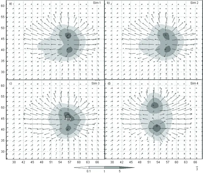
Fig. 12. YZ vertical cross sections in the plane passing through maximum updraft value of RS in all simulations at 3120 s. Vectors represent the wind speed. At the bottom of the figure is a 3 m/s vector indication. The amount of rain (shaded areas), cloud + ice water (solid isolines) and hail (dotted isolines).
minimun value of W at surface calculated every 120s. The strongest updraft and lowest Wmin values are observed in Sim4. The rest of the simulations show the same Wmin distribution in time. The lowest clouds formed in Sim1 while in the rest of the simulations no appreciable difference was observed. The wind shear above 10 km seems to act as a dynamic barrier to the cloud development in this case. A vertical cross section of clouds in the yz plane passing through maximum updrafts in each simulation is shown in Figure 12 (at 3120 s), where the aforementioned difference in cloud top among simulations can be seen. Sim1 shows the largest difference between the two storms, while the symmetry increases from Sim1 to Sim 4.
39
30 33 36 42 45 48 51 54 57 60 63 30 33 36 39 42 45 48 51 54 57 60 63
0.1 1 5
3
a) b)
c) d)
18000
16000
14000
12000
10000
8000
6000
4000
2000
0 18000
16000
14000
12000
10000
8000
6000
4000
2000
As the wind shear is removed in Sim4, the high perturbation pressure region above the 8 km (explained in section 4.1) decreases substantially with the consequent decrease of the negative pressure gradient that acted against the LS updraft development (Fig. 13a). For this reason, the storms simulated in Sim2 and 3 present a larger symmetry than those in Sim1, although some asymmetry is still observed due to the entrainment of drier and colder air at midlevels into the left storm’s updraft (explained in section 4.1). As the wind shear is removed at all heights in Sim4, the entrainment consists mainly of environmental air favoring the same development in both storms (Fig. 13b). Thus, the mechanisms that inhibited the development of the LS in Sim1 were not present in Sim4, favoring its development.
The life cycle of the storms was approximately the same in Sim1, 2 and 3. However, it was slightly shorter in Sim 4. Houston and Wilhelmson (2002) suggest that updraft maintenance is related to the fluid shear term associated with the tilted environmental vorticity and in Sim4 that term is null.
5. Summary and conclusions
The structure and main physical mechanisms of the convection developed on 21 july 2001 in the eastern region of Cuba was studied with the ARPS model and a sounding that provided the initial basic state. The 1800 UTC sounding of that day was used to initialize the simulation, whose hodograph presented a small clockwise turning with height at low and midlevels and a strong unidirectional wind shear at higher levels. It was evidenced that a local environment as that provided by the Fig. 13. a) Vertical cross section passing through the plane (x = 53.5 km) of maximum updrafts in both clouds at 2880 s. The contours represent the pressure perturbation and the shaded areas the vertical velocity. b) The same as in Fig. 6 for Sim 4 at 3000 s.
18000
3 0 3 3 3 6 3 9 4 2 4 5 4 8 5 1 5 4 5 7 4 0
5 0
4 4 4 6 4 8 5 2 5 4 5 6 5 8 6 0 6 2 1 0
44
42
40
38
36
32 34 50
48
46 56
54
52
10
5
1
0
a)a)
a ) b)
16000
2000 4000 6000 8000 10000 12000 14000
sounding was favorable for a storm splitting, with two split storms that moved to the right and to the left of the mean wind at low levels. Other simulations using axial symmetric initial bubble and the same sounding were made to reaffirm that split occured independent from the shape of bubble. The RS reached a larger development than the LS, whose development was inhibited. Furthermore, hail was observed in most of the simulation but larger amounts of hail reached the surface after the splitting in the RS.
Two mechanisms were responsible for the inhibition of the left-moving storm. The first is the vertical pressure gradient (maximum pressure values at higher levels and minimum pressure values at low levels) that acted against the main updraft development, possibly due to the strong shear present at higher levels. The second cause is the entrainment of drier and colder air in the LS’s updraft at midlevels coming from the downdraft region, while moister environmental air is entrained into the RS’s updraft.
High CAPE and moisture values normally exist in the study region, which influences the development of strong deep convection. However, as the formation of hailstorms is not very common, the wind profile measured at the surface station was studied to determine its influence on the convection that developed that day and the generation of hail at surface. For that reason, a further sensitivity study of the wind profile on the severity of the simulated storms was performed with three additional simulations. Several parameters were selected to compare the severity.
The wind shear above 10 km was favorable for a larger hail production, intensity and maximum hail at the surface. It is possibly related to the storm-relative flow at the anvil level that drags the slowly falling hydrometeors (the lightest ones) away from the updraft thus preventing them from reentering into the updraft. It produces less competition for the liquid water available between hydrometeors within the updraft allowing hail stones to grow to larger sizes and become the dominant kind of precipitation (Rasmussen and Straka, 1998). Furthermore, the area of precipitation decrease at the surface when the wind shear above10 km is removed because of the reduced extent of anvil. When the wind shear below 7 km was also removed (Sim 4), the total volume of precipitation (Vpr), maximum horizontal winds, updrafts and the intensity of precipitation were the largest. The mean hail mixing ratio (Mqh) presented the same value as in Sim1. Due to the absence of the wind shear, the LS was not inhibited and both storms reached the same strength. This could be the reason why Vpr and Mqh were larger in this simulation, since in the other simulations Mqh and Vpr were produced mainly by the RS. The mechanisms mentioned above that inhibit the LS development were not present in this simulation.
The life cycle of the storms was approximately the same in the four simulations, but slightly shorter in Sim4, suggesting that the wind in the lower levels contributed to longer lasting storms. In Sim4 the maximum vorticity centers did not coincide with the main updrafts at lower levels, and this distribution did not contribute to the maintenance of the updrafts.
Some factors had a great impact on the results of this study. The small differences observed in the simulated storms were not influenced by the large bubble used to trigger convection. In other simulations where smaller perturbations were used, the storm intensity was proportional to the initial perturbation. However, the sensitivity to the different wind profiles among storms initiated with the same bubble remained independent from the initial perturbation value. On the other hand, the sounding was taken several km away from the region where strong convection and hail was observed and was taken several hours earlier. Thus, the homogeneous initial state provided by the sounding may not accurately represent the time storm environment. However, the current numerical simulation study showed that a local environment defined by the given sounding could be favorable for a specific kind of convection as well as the development of a hailstorm.
References
Barnes S. L., 1970. Some aspects of a severe right-moving thunderstorm deduced from mesonetwork
rawinsonde observations. J. Atmos. Sci. 27, 634-648.
Davies-Jones, R. P., 1985. Dynamical interaction between an isolated convective cell and a veering environmental wind field. Preprints, 14th Conf. on Severe Local Storms, Indianapolis, IN, Amer. Meteor. Soc. 216-219.
Fovell R. G. and Y. Ogura, 1989. Effect of vertical wind shear on numerically simulated multicell
storm structure. J. Atmos. Sci.46, 3144-3176.
Fovell R. G. and P.-H. Tan, 1998. The temporal behavior of numerically simulated multicell-type
storms. Part II: The convective cell life cycle and cell regeneration. Mon. Wea. Rev.126, 551-577.
Grass L. D., 2000. The dissipation of a left-moving cell in a severe storm environment. Mon. Wea.
Rev. 128,2797–2815.
Houze R. A., Jr., 1993. Cloud Dynamics. Academic Press, San Diego, 573 p.
Houston A. and R. B. Wilhelmson, 2002. Numerical simulation of storm-boundary anchoring in a high-CAPE, low-shear environment: Implications for the modulation of convective mode. Preprints,
21st Conf. on Severe Local Storms,San Antonio, TX, Amer. Meteor. Soc., 345-348.
Klemp J. B. and R. B. Wilhelmson, 1978a. The simulation of three-dimensional convective storm
dynamics.J. Atmos. Sci.35,1070-1096.
Klemp J. B. and R. B. Wilhelmson, 1978b. Simulations of right and left moving storms through
storm splitting. J. Atmos. Sci.35, 1097-1010.
Lin Y. L., R. D. Farley and H. D. Orville, 1983. Bulk parameterization of the snow field in a cloud
model.J. Clim. Appl. Meteor.22, 1065-1092.
McCaul E. W. Jr. and M. L. Weisman, 2001. The sensitivity of simulated supercell structure and
intensity to variations in the shapes of environmental bouyancy and shear profiles. Mon. Wea.
Rev.129, 664-687.
Rasmussen E. N. and J. M. Straka, 1998. Variations in supercell structure. Part I: Observations of
the role of upper-level storm-relative flow. Mon. Wea. Rev.126, 2406-2421.
Rotuno R. and J. B. Klemp, 1985. On the rotation and propagation of simulated supercell
Schlesinger R. E., 1978. A three-dimensional numerical model of an isolated thunderstorm. Part I:
Comparative experiments for variable ambient windshear. J. Atmos. Sci.35, 690-713.
Schlesinger R. E., 1980. A three-dimensional numerical model of an isolated thunderstorm. Part II:
Dynamics of updraft splitting and mesovortex couplet evolution. J. Atmos. Sci.37, 395-420.
Weisman M. L. and J. B. Klemp, 1984. The structure and classification of numerically simulated
convective storms in directionally varying wind shears. Mon. Wea. Rev.112, 2479-2498.
Wilhelmson R. B. and J. B. Klemp, 1978. A numerical study of storm splitting that leads to
long-lived storms. J. Atmos. Sci.35, 1974-1986.
Wilhelmson R. B. and J. Klemp, 1981. A three-dimensional numerical simulation of splitting severe
storms on 3 april 1964. J. Atmos. Sci.38, 1581-1600.
Xu Q., M. Xue and K. K. Droegemeier, 1996. Numerical simulations of density currents in sheared
environments within a vertically confined channel. J. Atmos. Sci.53,770-786.
Xue M., K. K. Droegemeier, V. Wong, A. Shapiro and K. Brewster, 1995. ARPS Version 4.0 User’s Guide. Available from Center for Analysis and Prediction of Storms, University of Oklahoma, Norman, OK 73072. 380p.
Xue M., K. K. Droegemeier and V. Wong, 2000. The Advanced Regional Prediction System (ARPS) - A multiscale nonhydrostatic atmospheric simulation and prediction tool. Part I: Model dynamics
and verification. Meteor. Atmos. Phys. 75, 161-193.
Xue M., K. K. Droegemeier, V. Wong, A. Shapiro, K. Brewster, F. Carr, D. Weber, Y. Liu and D.-H. Wang, 2001. The Advanced Regional Prediction System (ARPS) - A multiscale nonhydrostatic
atmospheric simulation and prediction tool. Part II: Model physics and applications. Meteor.
Atmos. Phys. 76, 134-165.
Xue M., D.-H. Wang, J.-D. Gao, K. Brewster and K. K. Droegemeier, 2003. The Advanced Regional Prediction System (ARPS), storm-scale numerical weather prediction and data