Income and beyond: multidimensional poverty in six Latin American countries

C

C

|

E

_E

|

D

_D

|

L

_L

|

A

_A

|

S

_S

Centro de Estudios

Distributivos, Laborales y Sociales

Maestría en Economía Universidad Nacional de La Plata

Income and Beyond: Multidimensional Poverty in

Six Latin American countries

Diego Battiston, Guillermo Cruces, Luis Felipe Lopez

Calva, Maria Ana Lugo y Maria Emma Santos

Queen Elizabeth House (QEH), University of Oxford

1

Centro de Estudios Distributivos Laborales y Sociales (CEDLAS), Universidad Nacional de La Plata, Argentina

2

Centro de Estudios Distributivos Laborales y Sociales (CEDLAS)-Universidad Nacional de La Plata (UNLP) andConsejo

Nacional de Investigaciones Cientificas y Técnicas (CONICET), Argentina.

3_{United Nations Development Programme, Regional Bureau for Latin America and the Caribbean.}

4_{Department of Economics, University of Oxford, Manor Road Building, Manor Road, Oxford, OX1 3UQ}

5

Oxford Poverty and Human Development Initiative (OPHI), Oxford University andConsejo Nacional de Investigaciones

Científicas y Técnicas (CONICET)-Universidad Nacional del Sur, Argentina. Correspondence to: maria.santos@qeh.ox.ac.uk.

This study has been prepared within the OPHI theme on applications of multidimensional poverty measurement.

OPHI gratefully acknowledges support for its research and activities from the Government of Canada through the International Development Research Centre (IDRC) and the Canadian International Development Agency (CIDA), the Australian Agency for International Development (AusAID), and the United Kingdom Department for International Development (DFID)

ISSN 2040-8188 ISBN 978-1-907194-13-9

OPHI

W

ORKING

P

APER

N

O

. 17

Income and Beyond:

Multidimensional Poverty in six Latin American countries

Diego Battiston

_{, Guillermo Cruces}

_{, Luis Felipe Lopez Calva}

_,

Maria Ana Lugo

_{and Maria Emma Santos}

September 2009

Abstract

This paper presents empirical results of a wide range of multidimensional poverty measures for: Argentina, Brazil, Chile, El Salvador, Mexico and Uruguay, for the period 1992–2006. Six dimensions are analysed: income, child attendance at school, education of the household head, sanitation, water and shelter. Over the study period, El Salvador, Brazil, Mexico and Chile experienced significant reductions of multidimensional poverty. In contrast, in urban Uruguay there was a small reduction in multidimensional poverty, while in urban Argentina the estimates did not change significantly. El Salvador, Brazil and Mexico together with rural areas of Chile display significantly higher and more simultaneous deprivations than urban areas of Argentina, Chile and Uruguay. In all countries, access to proper sanitation and education of the household head are the highest contributors to overall multidimensional poverty.

Keywords: Multidimensional poverty measurement, counting approach, Latin America, Unsatisfied Basic Needs, rural and urban areas.

The Oxford Poverty and Human Development Initiative (OPHI) is a research centre within the Oxford Department of International Development, Queen Elizabeth House, at the University of Oxford. Led by Sabina Alkire, OPHI aspires to build and advance a more systematic methodological and economic framework for reducing multidimensional poverty, grounded in people’s experiences and values.

This publication is copyright, however it may be reproduced without fee for teaching or non-profit purposes, but not for resale. Formal permission is required for all such uses, and will normally be granted immediately. For copying in any other circumstances, or for re-use in other publications, or for translation or adaptation, prior written permission must be obtained from OPHI and may be subject to a fee.

Oxford Poverty & Human Development Initiative (OPHI) Oxford Department of International Development Queen Elizabeth House (QEH), University of Oxford 3 Mansfield Road, Oxford OX1 3TB, UK

Tel. +44 (0)1865 271915 Fax +44 (0)1865 281801

ophi@qeh.ox.ac.uk http://ophi.qeh.ox.ac.uk/

The views expressed in this publication are those of the author(s). Publication does not imply endorsement by OPHI or the University of Oxford, nor by the sponsors, of any of the views expressed.

Acknowledgements

This study was supported by the United Nations Development Programme Regional Bureau for Latin America and the Caribbean, and the Oxford Poverty and Human Development Initiative, University of Oxford. The authors are thankful for comments provided by Andrés Ham as well as by participants of OPHI Seminars Series in Trinity Term 2009, and of the third Meeting of the Society for the Study of Economic Inequality (ECINEQ), Buenos Aires, 21–23 July, 2009. The authors also thank Felix Stein for research assistance.

Acronyms

AF Alkire and Foster

BC Bourguignon and Chakravarty

CES Constant Elasticity of Substitution

ECLAC Economic Commission for Latin America and the Caribbean

FGT Foster Greer and Thorbecke

1. Introduction

There is a longstanding literature on poverty analysis in the region, based both on the Unsatisfied Basic Needs (UBN) approach and on income poverty. The former approach was promoted in the region by the Economic United Nation’s Economic Commission for Latin America and the Caribbean (ECLAC) and used extensively since at least the beginning of the 1980s (Feres and Mancero, 2001). The latter was spurred by the relatively early development of calorie consumption-based national poverty lines derived from consumption and expenditure surveys (Altimir, 1982).

Most commonly, the UBN approach combines population census information on the condition of households (construction material and number of people per room), access to sanitary services, education and economic capacity of household members (generally the household head). The UBN indicators are often reported by administrative areas in terms of the proportion of households unable to satisfy one, two, three, or more basic needs, and are often presented using poverty maps. Thus, in practice, the approach does not offer a unique index but rather the headcounts associated with the number of basic needs unmet. Among other things, the approach has been criticized for its crude aggregation index.

In a context where household surveys were not as widespread as nowadays and income and consumption were difficult variables to measure, the census-based UBN measures became the poverty analysis tool par excellence in the region, while income poverty studies were restricted to specific surveys and individual studies (Gasparini, 2004).1 _{However, as household surveys started to be regularly}

administered and progressively available to the public, distributional studies using income gained increasing attention and – in a way – displaced the UBN approach.

With the increased popularity of the income approach, income poverty measures based on national and international poverty lines started to be routinely reported by statistic institutes and research centers from the region, and scores of studies employ this information. However, most databases and studies tend overwhelmingly to focus on the poverty headcount, that is, the same crude aggregation methodology used by the UBN approach.2

Recovering interest in the multidimensionality of poverty, highlighted early in the region by the UBN approach, this study aims to provide estimates of poverty beyond the income dimension for countries in Latin America. However, this is done using a more sophisticated approach to the combination of these multiple dimensions, based on sound principles of distributive analysis. By promoting a multidimensional approach to poverty measurement, the paper is also attuned to the current needs of tools for targeting social programmes.3

The results below attempt to fill the gap in the literature by presenting a multi-country analysis of multidimensional poverty based on the latest development in poverty measurement. The existing studies

1_{Household surveys did not become regular until the 1970s or even later in Latin American countries and even when they}

were performed, micro-datasets were not publicly available for researchers.

2 _{A series of income-based poverty measures and unsatisfied basic needs indicators for most countries in the region are}

computed regularly and available online through the Socio-Economic Database for Latin America and the Caribbean (CEDLAS and World Bank, 2009). This is one of the few exceptions, reporting not only income poverty headcounts but also the poverty gap and the squared poverty gap for each survey (Foster, Greer and Thorbecke, 1984).

3_{Indeed the identification of the beneficiaries of the Progresa/Oportunidades (Conditional Cash Transfer Program) uses}

in this specific area are limited in the region. Amarante et al. (2008) and Arim and Vigorito (2007) present a similar analysis for Uruguay, while others used data from countries in the region to illustrate different methodological developments – Paes de Barros et al. (2006) for Brazil, Conconi and Ham (2007) for Argentina, Ballon and Krishnakumar (2008) for Bolivia. Lopez-Calva and Rodriguez-Chamussy (2005), and Lopez-Calva and Ortiz-Juarez (2009) have also adopted a multidimensional approach to studying poverty in Mexico, estimating the magnitude of the exclusion error when a monetary measure (vs. a multidimensional one) is adopted.

In summary, the contribution of this study is twofold. On the one hand, it presents a discussion of the application of multidimensional poverty measures in the context of Latin America. On the other hand, it presents results from six countries (Argentina, Brazil, Chile, El Salvador, Mexico and Uruguay) based on comparable data sources and indicators.

The rest of the paper is organised as follows. Section 2 briefly discusses the existing approaches to multidimensional poverty. Section 3 describes the poverty measures selected for this study. Section 4 presents the dataset, the selected dimensions, the indicators, thresholds and the weights employed in the analysis. Section 5 presents the empirical results, and Section 6 provides some concluding remarks.

2. Approaches to multidimensional poverty

In recent years, a consensus has emerged among those studying and making policies related to individuals’ well-being: poverty is best understood as a multidimensional phenomenon. However, views differ among analysts regarding the relevant dimensions and their relative importance. Welfarists stress the existence of market imperfections or incompleteness and the lack of perfect correlation between relevant dimensions of well-being (Atkinson 2003, Bourguignon and Chakravarty 2003, Duclos and Araar 2006), which makes the focus on a sole indicator such as income somewhat unsatisfactory. Non-welfarists point to the need to move away from the space of utilities to a different and usually wider space, where multiple dimensions are both instrumentally and intrinsically important. Among the non-welfarists, there are two main strands: the basic needs approach and the capability approach (Duclos and Araar 2006). The first approach, based on Rawls’ Theory of Justice, focuses on a set of primary goods that are constituent elements of well-being and considered necessary to live a good life (Streeten et al. 1981). The second approach, championed by Sen (1992), argues that the relevant space of well-being should be the set of functionings (or outcomes) that the individual is able to achieve. This set is referred to as the capability set “reflecting the person’s freedom to lead one type of life or another” (Sen 1992, p. 40).4

Rooted in different theoretical understandings of what constitutes a good life, all three approaches face the same problem: if well-being and deprivation are multidimensional, how should we make comparisons between two distributions and assess, for instance, whether one distribution exhibits higher poverty levels than the other? To answer this question one needs to make decisions about the domains relevant to well-being, their respective indicators and threshold levels, and the aggregation function (if completeness is desired). While these choices might differ substantially across approaches, in the present paper a single choice of dimensions, indicators and thresholds is considered and the focus is placed instead on the different aggregation forms.5 _{In particular, we compare the results obtained using the}

multidimensional poverty measure proposed by Alkire and Foster (2007), built in the spirit of the capability approach, with the indices proposed by representatives of the two other perspectives: the Bourguignon and Chakravarty (2003) measure and the Unsatisfied Basic Needs index.

4_{See Duclos and Araar (2006) for a thorough analysis of the differences between the three approaches.}

The UBN approach has been criticized on several grounds, specifically regarding the (arbitrary) selection of the indicators, the (arbitrary) implicit weights, the identification methodology and the aggregation index, which uses headcounts. Overcoming some of these deficiencies, Alkire and Foster (2007) (AF from here onwards) propose a family of measures which combine information on both the number of deprivations and their level, and – when data are cardinal – information on poverty depth and distribution can be incorporated also. The family is an extension of the FGT class of measures (Foster, Greer and Thorbecke, 1984) and satisfies a set of desirable properties. In addition, the AF measures also allow for different dimension weighting schemes. The approach uses a dual cut-off – one for each dimension, and one for the number of dimensions k required to be considered poor. Therefore, a household is described as poor if it is deprived in k or more dimensions. A key feature of one of the measures in the family is that it allows qualitative and quantitative information to be combined. Thus census information (such as dwelling characteristics and access to services) and income or consumption data can be aggregated in a meaningful way.

At the same time, when using quantitative information (i.e. continuous variables), one might be interested in incorporating the idea that dimensions of deprivation are to some extent substitutes (or complements). In other words, high deprivations in one dimension can be compensated by lower deprivations in another one. Bourguignon and Chakravarty (2003) (referred to as BC hereafter) suggest a family of multidimensional poverty measures which is also a generalization of the FGT family of measures, but that aggregates relative deprivations using a Constant Elasticity of Substitution (CES) function, implying a degree of substitution between dimensions.

The following pages describe these three groups of measures – the UBN, the AF and the BC measures. The empirical results below present estimates of these measures, as well as deprivation rates by dimension, for Argentina, Brazil, Chile, El Salvador, Mexico and Uruguay at five different points in time between 1992 and 2006, using two alternative weighting systems.

3. Multidimensional poverty indices

The construction of a poverty measure involves two steps (Sen, 1976): first, the identification of the poor; second, the aggregation of the poor. In the unidimensional income approach, the identification step defines an income poverty line based on the amount of income that is necessary to purchase a basic basket of goods and services. Individuals and households are thus identified as poor if their income (per capita or adjusted by the demographic composition of the household) x_i falls short of the poverty line

z. The individual poverty level is generally measured by the normalized gap defined as:

(1)

  

 

 



z x for g

z x for z

x z g

i i

i i

i 0

] / ) [(

The individual information is most commonly aggregated in the second step using the aggregation function proposed by Foster, Greer and Thorbecke (1984) known as the FGT measures, defined as:

(2)

1

1 

 





i

FGT g

n

equally. When  1, the measure is the poverty gap, where individuals’ contribution to total poverty depends on how far away they are from the poverty line, and with  2, the measure is the squared poverty gap, where individuals receive higher weight the larger their poverty gaps are. For  0 the measure satisfies monotonicity (i.e. it is sensitive to the depth of poverty); while for  1, it satisfies transfer (i.e. it is sensitive to the distribution among the poor).6

In the multidimensional context, distributional data are presented in the form of a matrix of size n d ,

d n

X , , in which the typical element x_ijcorresponds to the achievement of individual i in dimension j,

with i1,....,n and j1,....,d. Following Sen (1976), one is first required to identify the poor. The most common approach is to first define a threshold level for each dimensionj,below which a person is considered to be deprived. The collection of these thresholds can be expressed in a vector of poverty linesz(z₁,....,z_d). In this way, whether a person is deprived or not in each dimension is defined. However, unlike unidimensional measurement, a second decision needs to be made in the multidimensional context: among those who fall short in some dimension, who is to be considered multidimensionally poor? A natural starting point is to consider all those deprived in at least one dimension, the so called union approach. However, more demanding criteria can be used, even to the extreme of requiring deprivation in all considered dimensions, the so called intersection approach. In terms of Alkire and Foster (2007), this constitutes a second cut-off: the number of dimensions in which someone is required to be deprived so as to be identified as multidimensionally poor. The authors name this cut-off k. If c_i is the number of deprivations suffered by individual i, then she will be considered multidimensionally poor if c_ik.7

Once the process of identification of the multidimensionally poor has been solved, the aggregation step comes next. The measures described in what follows are multidimensional extensions of the FGT family of measures. For simplicity in the exposition, it is assumed that each selected dimension has only one indicator. This becomes relevant to the weighting structure discussed in Section 4 below.

3.1 The Multidimensional Headcount and the Unsatisfied Basic Needs Approach

The simplest extension of the FGT family of indices is the multidimensional headcount. Once the k cut-off value has been selected, it is straightforward to calculate the fraction of the population deprived in k

or more dimensions. Formally, this can be expressed as:

(3)

n q k

g n

z X H

n

i d

j

ij  

  

 



 

 

0

1 1

) ( 1

) ; (

where g_ij(k) is the censored poverty gap of individual i in dimension j, such that





ij k z x z

g ( ) (  )/ if xij zjand ci k, and gij(k)0otherwise, it is the number of people

deprived in kor more dimensions (q) over the total population (n). This measure is the one used by the Unsatisfied Basic Needs Approach (UBN), with the union approach (k 1) as the most common identification criterion.

6_{Foster (2006) provides a recent survey of axioms in unidimensional poverty measurement.}

7_{Another approach would be to first define an aggregate of well-being for individual i and then define the poverty threshold}

in the space of the well-being metric, which can be a function of the dimension specific poverty thresholds (z(z1,....,zd)).

One implication of the approach is that households are described by counting the number of deprivations suffered. This implies that each indicator is weighted equally, irrespective of its nature and the number of indicators used to describe each dimension. If there is more than one indicator corresponding to the same dimension, this means that some dimensions are weighted disproportionately more than others (Feres and Mancero, 2001). Secondly, as pointed out by Alkire and Foster (2007), the multidimensional headcount is not sensitive to the number of deprivations that the multidimensionally poor experience; that is, it violates what the authors call dimensional monotonicity. Given a k value, unless the intersection approach is used (kd) if an individual identified as poor becomes deprived in an additional dimension, the multidimensional headcount does not change. Thirdly, in line with traditional critiques of the headcount in the unidimensional space, it ignores all information over the extent of deprivation. Thus, the UBN approach is not able to account for the extent and severity of poverty.8 Finally, although it is possible to decompose the headcount in subgroups of population, it is not possible to distinguish the contribution of each dimension to overall poverty. The following families of indices account for these problems.

3.2 Alkire and Foster (2007) family of indices: the Mα measures

Using the dual cut-off approach previously explained for the identification of the multidimensionally poor, Alkire and Foster (2007) propose the dimension adjusted FGT measures, or Mα family of measures, given by the following expression:

(3)







 

 n

i d

j

ij j g k w nd

z X M

1 1

) ( 1

) ;

( 

 with  0

where g_ij(k)is the censored poverty gap of individual iin dimension j, as defined in the previous

section; w_jis the weight assigned to dimension j , such that





d

j

j d w

1

, and α is the parameter of

dimension-specific poverty aversion. It is worth noting that the weighting system affects not only aggregation but also identification. When equal weights are used, (w_j 1 for all j1,...,d), the identification cut-off ranges from k=1, corresponding to the union approach, to k=d, corresponding to the intersection approach, and someone is multidimensionally poor when her number of deprivations is equal or greater than k: c_ik. When ranking weights are used, so that some dimensions receive higher weights than others, c_i becomes the weightednumber of deprivations in which the individual is deprived.9

In this case, the minimum possible k value, which corresponds to the union approach, is given by the minimum weight: k=min(w_j), while the maximum possible kcut-off value remains to be d.10

Similar to the unidimensional FGT measures, three members of this family are worth mentioning. When 0



 , the measure is the adjusted headcount ratio. It can be shown that it is the product of the multidimensional headcount ratio H (defined in expression 2) and the average deprivation share across

8_{Another criticism is that, in practice, UBN measures are considered more “structural”, since they are not sensitive to}

short-run spells of poverty due to the exclusion of variables such as income and consumption. UBN measures also tend to underestimate urban poverty since deprivations related to the dwelling and access to sanitary services tend to be lower in urban areas. We do not stress these points in the paper given that they are the direct consequences of the dimensions and indicators chosen and not the way indicators are aggregated, the focus of this section.

9_{For example if an individual is deprived in income and health, and income has a weight of 2, while health has a weight of}

0.5, then ci 2.5 and not 2, as it would be with equal weights.

10_{The Mα family of measures is presented in Alkire and Foster (2007) as the mean of the censored matrix of normalised alpha}

the poor A (M0 HA), where A is given by /( ) 1 qd c A n i i



 . The A measure indicates the fraction of the d

dimensions in which the average multidimensionally poor individual is deprived. In this way, M0has an

advantage over the multidimensional H: it is sensitive to the number of deprivations the multidimensionally poor experience, i.e. it satisfies dimensional monotonicity (Alkire and Foster, 2007, p. 16). When  1, the measure is the adjusted poverty gap, defined as the weighted sum of dimension-specific poverty gaps. This measure is not only sensitive to the number of deprivations the poor experience but also to their depth, that is, it satisfies monotonicity. Finally, when  2 the measure is the adjusted squared poverty gap, defined as the weighted sum of the dimension-specific squared poverty gaps. This measure satisfies the two types of monotonicity mentioned above, and it is also sensitive to the inequality of deprivations among the poor, satisfying the multidimensional transfer property.11

In addition to the aforementioned properties, all members of the M_α family can be decomposed by subgroups of population and by dimensions. Given a population subgroup I, its contribution to overall poverty is given by:

(4)   M M n n

C I I

I 1             

where (n_I /n) and M_I are the population share and the poverty measure of subgroup I respectively, and Mis the poverty measure for the overall population. Moreover, once the identification step has been completed, all members of the M_α family can be decomposed into the contribution of each dimension.12Specifically, the contribution of dimension J is given by

(5)





  M k g nd C n i iJ J 1 ) ( 1 1             



These two decompositions will be used in the results presented below to unveil the composition of the multidimensional poverty observed and their evolution, and to highlight the differences across countries.

3.3 Bourguignon and Chakravarty (2003) family of indices

Bourguignon and Chakravarty (2003) adopt a union approach for the identification of the multidimensionally poor. In terms of the second cut-off parameter specified in the previous subsection, this means that they use a value of k = 1, so that a person is considered to be multidimensionally deprived as long as she falls short in any of the considered dimensions. In terms of the identification step, Bourguignon and Chakravarty’s (2003) family of measures constitutes a special case of Alkire and Foster’s (2007). However, as shown below, in terms of the aggregation step the opposite is true. The

11_{Alkire and Foster (2007) show that that}

1

M is the product of the multidimensional headcount H, the average deprivation

share across the poor A, and the average poverty gap G among the poor (M₁ HAG), where G is given by









ij k g k

g G 1 1 0 1 1 ) ( / )

( . Analogously, the authors express M2 as the product of the multidimensional

headcount H, the average deprivation share across the poor A, and the average severity of deprivations among the poor S

(M2HAS), where S is given by









           





ij k g k

g S 1 1 0 1 1 2 ) ( / ) ( .

12 _{Strictly speaking, because the identification step needs to be completed in the first place, this is not a decomposability}

interaction between these families of measures is related to the core of the discussion in the contemporary literature on multidimensional poverty and well-being: the interrelation between dimensions and its implication for poverty measurement.

The relationship between dimensions becomes relevant for poverty measurement under a specific type of transfer or rearrangement, called correlation increasing switch by Bourguignon and Chakravarty (2003).13

Given two poor individuals A and B, with A having strictly higher achievements than B in some dimensions, but strictly lower achievements in others, there is a transfer between the two that makes one of them – say A – end up having higher achievements in alldimensions and hence the correlation (or the association) between dimensions has increased as a result of it. What should happen to the poverty measure in such a case? If dimensions are thought to be substitutes, poverty should not decrease, whereas if dimensions are thought to be complements, poverty should not increase.14 _{These two}

properties are referred to by Bourguignon and Chakravarty (2003) as ‘Non-Decreasing Poverty under Correlation Increasing Switch’ (NDCIS), and ‘Non-Increasing Poverty under Correlation Increasing Switch’ (NICIS), respectively. There is also scope for dimensions to be considered independent, in which case, poverty should not change under the described transformation. It should be mentioned that the substitutability, complementarity or independence relationship between dimensions is defined in this literature in terms of the second cross partial derivative of the poverty measure with respect to any two dimensions being positive, negative or zero, respectively. This corresponds to the Auspitz-Lieben-Edgeworth-Pareto (ALEP) definition, and differs from Hick’s definition traditionally used in the demand theory (which relates to the properties of the indifference contours) (Atkinson, 2003, p. 55).15

The family of multidimensional poverty indices proposed by Bourguignon and Chakravarty (2003) aggregates shortfalls across dimensions for each individual using a constant elasticity of substitution function that allows for different degrees of substitutions to be incorporated, and then aggregates across individuals’ multidimensional deprivations using the standard FGT formula. The family of indices is then given by:

(4)

 





              n i d j ij j g d w n z X P 1 / 1 ) 1 ( 1 ) ; (    

 with  0and  1

Following the previous notation, g_ij(1) is the censored poverty gap of individual iin dimension j,using a cut-off value of k=1 and whenw_j and d are defined as above. The parameter  measures the degree of aversion to multidimensional poverty, with higher values attaching a higher weight to individuals with higher multidimensional deprivation. Note that in AF the parameter α measures the level of aversion to

dimension-specific poverty while in BC it measures the aversion to multidimensional poverty. The  parameter measures the degree of substitutability between dimension shortfalls in the Hicks’ sense; the higher the θ, the lower the substitutability between dimensions. The value of θ is set to be equal or greater than one so that the standard convex – diminishing returns – assumption between dimensions is

13_{This type of transformation was first discussed by Atkinson and Bourguignon (1982) and Boland and Proschnan (1988). It}

was first introduced in the multidimensional inequality measurement by Tsui (1999) and multidimensional poverty measures by Tsui (2002). Alkire and Foster (2007) rename the term as association increasing rearrangement, since the term ‘association’ seems better suited than ‘correlation’, which refers only to a specific type of association. Seth (2008) provides further discussion on this issue.

14_{The intuition is that if dimensions are substitutes, before the transfer, both A and B were able to compensate their meagre}

achievements in some dimensions with their higher achievements in the others; after the transfer B is no longer able to do so, and therefore poverty should increase (or at least not decrease). On the other hand, if attributes are complements, before the transfer, neither A nor B were able to achieve a certain level of well-being since both were lacking in some dimension; after the transfer, at least A is able to do so.

satisfied.16 _For θ _{= 1 dimensions are perfect substitutes. At the extreme, for} θ → ∞_{, dimensions are}

perfect complements and individuals are judged according to their worst performance in any single dimension. In terms of the ALEP definition, dimensions are considered substitutes, complements or independent depending on the value of  relative to that ofθ. When α > θ, dimensions are considered substitutes, and the indices satisfy the NDCIS property, so that an increase in the association between dimensions does not decrease poverty. On the other hand, when α < θ, dimensions are considered complements, and the indices satisfy the NICIS property, so that an increase in the association between dimensions does not increase poverty. Finally, when α = θ dimensions are considered to be independent, and increases in the association between them do not affect the poverty measure.

Some members of the BC family of measures are worth noting. With α =0, independently of the value of θand of the weights used, the BC measure is reduced to the multidimensional headcount with k=1 and equal weights (UBN): P0(X;z)H(X;z).17Also, when the parameter of inequality aversion equals the degree of substitution between attributes, the BC measure coincides with the indices suggested by AF when k=1. Specifically, when θ = α = 1 the BC measure is the M1 measure: ( ; ) 1( ; )

1

1 X z M X z

P  ,

while, when θ = α = 2 the BC measure is the M2 measure: ( ; ) 2( ; ) 2

2 X z M X z

P  . In those cases, in which the two parameters α and θ coincide, dimensions are considered independent, and the poverty measure is insensitive to changes in the level of association between dimensions. Therefore, in terms of the aggregation procedure, the AF measures can be seen as a specific case of the BC measures.18

In general, note that for α> 0, and given that  1, the indices satisfy monotonicity, and for α >1 and

θ> 1, they satisfy the transfer requirement.19_{Moreover, all members of the family can be decomposed in}

subgroups of population, so that the contribution of each subgroup can be calculated in an analogous way to that presented for the Alkire and Foster (2007) measures. However, only in the case in which θ=

α, that is, when dimensions are considered independent, can the indices be decomposed into the contributions of each dimension. This points to a trade-off present in multidimensional measurement: the possibility of breaking down the aggregate measure by dimensions vs. allowing for sensitivity to changes in the level of association between attributes. While BC seem to lean towards allowing some type of interaction between dimensions – given the indubitable interrelation between dimensions of well-being such as income, education, and health – AF seem to prefer dimension-decomposability, given the usefulness of being able to identify each dimension’s contribution for policy purposes.

4. Datasets, dimensions, poverty lines and weights

The dataset used in the paper corresponds to the Socioeconomic Database for Latin America and the Caribbean

(SEDLAC), constructed by the Centro de Estudios Distributivos Laborales y Sociales (CEDLAS) and the World Bank. The dataset comprises household surveys of different Latin American countries which have been homogenised to make variables comparable across countries – the details of this process are covered in CEDLAS (2009). This first multi-country study on multidimensional poverty in the region

16_{As presented, the degree of substitution is assumed to be constant and the same for all pairs of attributes. This might be}

considered unsatisfactory when working when more than two dimensions. One alternative is to consider a nested approach in which two dimensions of several subsets of dimensions are aggregated using the same CES function with each subset having

a differentθ, and second, these subsets are combined using again the same expression. Another alternative suggested by the

authors is to allow the substitutability parameter to be a function of the achievements.

17_{This marks a difference with the AF family, since in that case, the M}

0measure satisfies dimension monotonicity and it is

sensitive to the weighting system used.

18

However, AF mention that their measure can be extended to a class that considers interrelationships among dimensions by

replacing the individual poverty function M(xi;z) by

 ( ; )]

[M x_i z .

concentrates on a subset of the available database to maximize the possibilities for comparison across time and between countries.20_{The study covers the following six countries: Argentina, Brazil, Chile and}

Uruguay, El Salvador and Mexico. Altogether, they account for about 64 per cent of the total population in Latin America in 2006.

The paper performs estimates at five points in time between 1992 and 2006 for each country. Full details of survey names and sample sizes can be found in Table A.1 in the Appendix. In the case of Argentina and Uruguay, the data are representative only of urban areas and correspond to the years 1992, 1995, 2000, 2003 and 2006 in Argentina, and to the years 1992, 1995, 2000, 2003 and 2005 in Uruguay. In the other four countries data are nationally representative, including information from both urban and rural areas. In Brazil, data corresponds to the years 1992, 1995, 2001, 2003 and 2006; in Chile to 1992, 1996, 2000, 2003 and 2006; in El Salvador to 1991, 1995, 2000, 2003 and 2005 and finally in Mexico, to the years 1992, 1996, 2000, 2004 and 2006. The definition of ‘rural areas’ by the surveys performed in each of these four countries is fairly similar.21_{In each country, only households with complete information on}

all variables and consistent answers on income were considered.22

The selection of dimensions was based on several factors. As mentioned earlier, Latin America has a strong tradition of using the UBN approach. This approach is often also called the ‘direct method’ to measure poverty, since it looks directly at whether certain needs are met or not, as opposed to the ‘indirect (or poverty line) method’, which looks at the income level and compares it to the income level necessary to achieve these needs (Feres and Mancero, 2001). It has been long argued that both methods capture partial aspects of poverty, that both the income dimension as well as the UBN indicators are relevant for assessing well-being, and that there are significant errors in targeting the poor (either of inclusion or exclusion) when only one of them is used.23 _{Therefore, in this paper, a ‘hybrid method’ is}

adopted, in which both an income indicator as well as indicators typically used in the UBN approach are selected.24

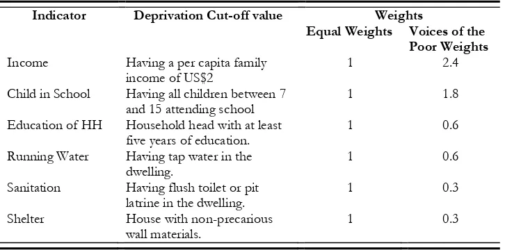
Table 1 presents the dimensions selected to perform the poverty estimates. For the income dimension, the World Bank’s poverty line of US$2 per capita per day was selected. It is acknowledged that this is a rather conservative poverty line for Latin America, but it guarantees full comparability across countries.25

Children’s education is another dimension considered, requiring all children between 7 and 15 years old

20_{The SEDLAC database (CEDLAS and World Bank, 2009) will report multidimensional poverty indicators systematically}

starting in 2009.

21_{In Chile it corresponds to localities of less than 1,000 people or with 1,000 to 2,000 people, of which most perform primary}

activities. In Mexico it refers to localities of less than 2,500 people. In Brazil, rural areas are not defined according to population size but rather they are all those not defined as urban agglomerations by the Brazilian Institute of Geography and Statistics. In El Salvador, rural areas are all those outside the limits of municipalities heads, which are populated centres where the administration of the municipality is located. Again, this definition does not refer to any particular population size.

22_{The Statistics Institute of each country has a criterion to identify invalid income answers (such as reporting zero income}

when working for a salary), which is incorporated in the SEDLAC dataset, as well as other types of invalid answers (such as reporting labour income when being unemployed).

23 _{Cruces and Gasparini (2008) illustrate these inclusion and exclusion effects by studying the targeting of cash transfer}

programs based on a combination of income and other UBN-related indicators.

24

This ‘hybrid method’ can be criticized of potential double-counting, arguing that dimensions that may have been considered in the basic consumption basket used to determine the poverty line are included again as a separate indicator. However, the spearman correlations between income and the other different indicators are relatively low (not exceeding 0.5 in any case) and decreasing over time, suggesting that a multidimensional approach does indeed incorporate new elements to poverty analysis.

25_{This poverty line is prior to the latest amendment by the World Bank (Ravallion, Chen and Sangraula, 2008), which raised}

(inclusive) to be attending school. This indicator belongs to the UBN approach. Households with no children are considered non-deprived in this indicator. A third indicator refers to the educational level of the household head, with the threshold set at five years of education. Again this indicator is part of the UBN approach, although in that approach (a) the required threshold is second grade of primary school and (b) it is usually part of a composite indicator together with the dependency index of the household (considered to be deprived if there are four or more people per employed member). Two years of education seemed a very low threshold, so five years were used instead. Also, given that the income indicator is being included, the high dependency index seemed less relevant in this hybrid approach. The other three indicators used relate to the dwelling’s conditions. The first two; having proper sanitation (flush toilet or pit latrine) and living in a shelter with non-precarious wall materials are typically included in the UBN approach.26_{The third indicator is having access to running water in the dwelling. Although}

this is not usually included in the UBN approach, it is considered important. In the absence of comparable health data, it can be seen as a proxy of this dimension, which is one of the most valued according to the participatory study performed in Mexico “Lo que dicen los pobres” (Székely, 2003)27_.

Table 1: Selected Indicators, Deprivation Cut-Off Values and Weights

Indicator Deprivation Cut-off value Weights

Equal Weights Voices of the Poor Weights

Income Having a per capita family

income of US$2

1 2.4

Child in School Having all children between 7

and 15 attending school

1 1.8

Education of HH Household head with at least

five years of education.

1 0.6

Running Water Having tap water in the

dwelling.

1 0.6

Sanitation Having flush toilet or pit

latrine in the dwelling.

1 0.3

Shelter House with non-precarious

wall materials.

1 0.3

Two alternative weighting systems are used.28_{The first scheme weights each indicator equally. However,}

if more than one indicator is associated with the same dimension, the equal weights are not really equal across dimensions. In this case, three of the indicators used refer to dwelling’s characteristics and two other indicators (children attending school and the education of the household head) refer to the dimension of education of the household. Therefore, the equal weights are implicitly weighting the dwelling conditions three times, and the education dimension twice, compared to the income dimension.

The second weighting structure is derived from a replica performed in Mexico – the participatory study on the voices of the poor – carried out by the country’s Secretaría de Desarrollo Social (Székely, 2003). In this study the poor were asked about their valuation of different dimensions. The number and variety of dimensions included in the questionnaire exceeds those considered here, however, its results are useful for producing a ranking of the six indicators. The new weighting scheme (last column in Table 1)

26_{In the UBN approach (and also in the Uruguay survey) the quality of shelter is defined in terms of “adequate shelter”.}

27 _{Clearly, using the same thresholds for both urban and rural areas is an arguable decision. One could imagine that the}

standards of what is ‘acceptable’ in a rural context (particularly in terms of sanitation, water and shelter) may differ from the standards in an urban context. However, from an ethical point, we see no strong reason why people in rural areas should conform to lower achievements in certain aspects of their living conditions than people in urban ones. We therefore deliberately require households in both areas to meet the same minimum requirements so as to be considered non-deprived. Additionally, this guarantees comparability across these areas.

28_{On the meaning of dimension weights in multidimensional indices of well-being and deprivation and alternative approaches}

gives the income dimension the highest weight, being 1.3 times the weight received by the children’s education, 4 times the weight received by the education of the household head and access to running water, and 8 times the weight received by having access to sanitation and proper shelter. These sets of weights will be referred to in what follows as voices of the poor weights (VP weights).

Three of the indicators are cardinal variables (income, proportion of children in the household not attending school and years of education of the household head) and three are dichotomous (having running water in the household, having proper sanitation and living in a house with non-precarious materials). When poverty measures other than the multidimensional headcount or the M0 measure are

estimated, equal weights assigns higher weight to the dichotomous variables than the continuous ones, because poverty gaps of all those that are poor are equal to 1. Applying measures that require cardinal data to a set of variables that include dichotomous ones is not technically correct. The only reason to do so is to obtain a rough sense of the depth and distribution of the deprivation in these dimensions. Also, when VP weights are used, the two variables that receive the highest weights (income and children in school) are continuous, shifting weight from dichotomous to cardinal variables, which lessens the problem.

5. Empirical results

5.1 Deprivation rates by dimension

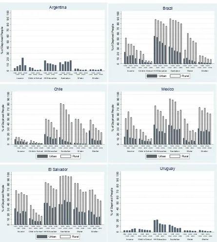
Figure 1 presents the deprivation rates for each dimension in each country and year, in rural and urban areas, except for Argentina and Uruguay where the rates correspond only to urban areas. Despite being a crude poverty measure, the headcount ratio for each dimension, country and year provides a preliminary picture of deprivation in the region. Comparing across countries and regions, one can distinguish two groups: the urban and rural areas of El Salvador, Mexico and Brazil together with the rural areas of Chile, and the urban areas of the southern cone countries – Argentina, Chile and Uruguay. The first group of countries and regions exhibit deprivation rates much higher than those in the second group, producing a sharp contrast. In particular, El Salvador is the country with the highest levels of deprivation in all dimensions. The deprivation rates in this country are high, not only in relative terms to those of the other countries, but also from an absolute point of view: in five out of the six indicators, the rural areas of the country presented deprivation rates of 50 per cent or higher in 2006. For most of the dimensions, deprivation headcounts in rural areas of El Salvador are followed by those of the rural areas of Brazil, Mexico and Chile, and then by the urban areas of El Salvador, Brazil and Mexico. Deprivation rates in the urban areas of Argentina, Chile and Uruguay are, for each dimension, well below those in the aforementioned regions. It is worth noting the disparities within countries between urban and rural areas: deprivation rates in rural areas are at least double urban deprivation rates. In Chile the difference is particularly marked, as if each of these areas – rural and urban – belonged to a different country.

Comparing across dimensions, three interesting features emerge. First, deprivations in the level of education of the household head and in sanitation are the dimensions with the highest headcount ratios in all six countries. They are extremely high in the rural areas of El Salvador, Brazil and Mexico where 70, 75 and 50 per cent of the population, respectively, lived in a household where the household head had less than 5 years of education in 2006 and 96, 80 and 68 per cent, respectively, lived in a household without access to proper sanitation facilities. Comparable deprivation rates in respective urban areas and in rural areas of Chile are between 22 and 45 per cent, whereas in the urban areas of Argentina, Chile and Uruguay they do not exceed 17 per cent. Second, in all countries, income deprivation lies in the middle of the rankings of deprivations, though rates vary significantly across countries (between 58 per

29_{Detailed and complete estimates of all measures, all k cut-offs and weights can be found in a companion document ‘WP 17}

cent in rural El Salvador to 3 per cent in urban Chile). Finally, it is worth noting that, although deprivation in the education level of the household head is one of the most prevalent deprivations in all countries, the percentage of families with at least one child that is not attending school is among the lowest deprivation rates. This is somewhat encouraging. If these low rates were to be sustained or – even better – decreased, future heads of households will be more educated than their parents and educational deprivation will cease to be as severe as at present.

Temporal trends are also encouraging. In almost all cases, deprivation rates declined between 1992 and 2006 and in many cases they were halved. The few exceptions are Uruguay, where income poverty steadily increased throughout the period, and Argentina, where poverty headcounts in income, sanitation and shelter are somewhat higher in 2006 than fifteen years before.30

30_{The evolution of the income poverty headcount reflects the increase of income poverty that the country registered during}

Figure 1: Deprivation Rates by Dimension Rural and Urban Areas, 1992-2006

0 1 0 2 0 3 0 4 0 5 0 6 0 7 0 8 0 9 0 1 0 0 % o f D e p ri v e d P e o p le

Income Child in School HH Education Sanitation Water Shelter

1992

19952000200320061992199520002003200619921995200020032006199219952000200320061992199520002003200619921995200020032006

Argentina 0 1 0 2 0 3 0 4 0 5 0 6 0 7 0 8 0 9 0 1 0 0 % o f D e p ri v e d P e o p le

Income Child in School HH Education Sanitation Water Shelter

1992

19952001200320061992199520012003200619921995200120032006199219952001200320061992199520012003200619921995200120032006

Brazil Urban Rural 0 1 0 2 0 3 0 4 0 5 0 6 0 7 0 8 0 9 0 1 0 0 % o f D e p ri v e d P e o p le

Income Child in School HH Education Sanitation Water Shelter

1992

19962000200320061992199620002003200619921996200020032006199219962000200320061992199620002003200619921996200020032006

Chile Urban Rural 0 1 0 2 0 3 0 4 0 5 0 6 0 7 0 8 0 9 0 1 0 0 % o f D e p ri v e d P e o p le

Income Child in School HH Education Sanitation Water Shelter

1992

19962000200420061992199620002004200619921996200020042006199219962000200420061992199620002004200619921996200020042006

Mexico Urban Rural 0 1 0 2 0 3 0 4 0 5 0 6 0 7 0 8 0 9 0 1 0 0 % o f D e p ri v e d P e o p le

Income Child in School HH Education Sanitation Water Shelter

1991

19952000200320051991199520002003200519911995200020032005199119952000200320051991199520002003200519911995200020032005

El Salvador Urban Rural 0 1 0 2 0 3 0 4 0 5 0 6 0 7 0 8 0 9 0 1 0 0 % o f D e p ri v e d P e o p le

Income Child in School HH Education Sanitation Water Shelter

1992

19952000200320061992199520002003200619921995200020032006199219952000200320061992199520002003200619921995200020032006

Uruguay

4.2. Multidimensional poverty: the multidimensional H and the M₀measure

The Multidimensional Headcount H and the Adjusted Multidimensional Headcount M₀ measures were estimated for k=1,…6, using the two weighting structures detailed above. This section focuses on the most relevant points that can be derived from these results.

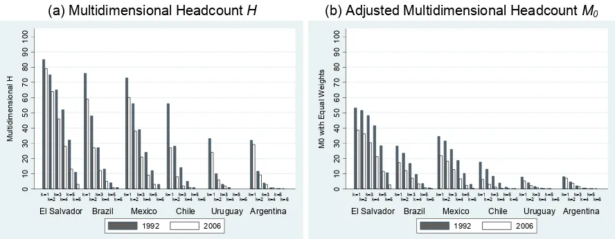
Figure 2 presents the multidimensional headcount (a) and adjusted headcount (b) for the different k

sorted according to their deprivation in 1992 when k=1. It is worth noting that the estimates in Argentina and Uruguay correspond only to urban areas.

Figure 2: Multidimensional Poverty for Different k_{Values and Equal Weights}

1992 and 2006

(a) Multidimensional Headcount H _{(b) Adjusted Multidimensional Headcount} M0

0 1 0 2 0 3 0 4 0 5 0 6 0 7 0 8 0 9 0 1 0 0 M u lt id im e n s io n a l H

El Salvador Brazil Mexico Chile Uruguay Argentina

k=1

k=2k=3k=4k=5k=6k=1k=2k=3k=4k=5k=6k=1k=2k=3k=4k=5k=6k=1k=2k=3k=4k=5k=6k=1k=2k=3k=4k=5k=6k=1k=2k=3k=4k=5k=6

1992 2006 0 1 0 2 0 3 0 4 0 5 0 6 0 7 0 8 0 9 0 1 0 0 M 0 w it h E q u a l W e ig h ts

El Salvador Brazil Mexico Chile Uruguay Argentina

k=1

k=2k=3k=4k=5k=6k=1k=2k=3k=4k=5k=6k=1k=2k=3k=4k=5k=6k=1k=2k=3k=4k=5k=6k=1k=2k=3k=4k=5k=6k=1k=2k=3k=4k=5k=6

1992 2006

Note: Estimates in Uruguay and Argentina correspond only to urban areas.

Among the countries for which data are available for both urban and rural areas, El Salvador is the poorest country, followed by Brazil, Mexico and then Chile. For k=1, Brazil has a higher H than Mexico in 1992, and about the same in 2006, but for higher kvalues, Mexico has much higher H. This suggests that deprivations in Mexico are more coupled than in Brazil: if one person fails to achieve an adequate level in a given indicator, it is more likely that she will also fall short in another indicator in Mexico than in Brazil.

Between 1992 and 2006, all countries reduced their multidimensional headcounts for all k values.31_Most

impressively, Chile halved its headcounts for all k values whereas El Salvador, Mexico and Brazil achieved this sort of reduction for higher k values (k≥4). In Argentina, the reduction in the multidimensional headcount was very mild and indicates that losses in some dimensions (such as income, shelter and sanitation) are being compensated by the gains in others (such as education and water)32

Using the adjusted headcount ratio M0, a measure sensitive to the breadth of poverty shown in (b) of

figure 2, the differences between El Salvador and the rest of the countries for which urban and rural data are available become sharper. Not only does it exhibit the highest multidimensional poverty levels, but it is also well above the estimates for the other countries, doubling or more the next highest estimate for all kvalues. Also, once the multidimensional headcount is adjusted it becomes more evident that Mexico is worse-off than Brazil; the average number of deprivations experienced by the poor in Mexico is higher relative to Brazil. In El Salvador, Mexico, Brazil and Chile, the declines inM₀are larger in relative terms than those in H, most notably for lower values of k. The interpretation of this is that not only that there are fewer deprived people at the end of the period but also that those that are deprived, experience fewer deprivations on average. In urban Uruguay, the reduction of M0was very small and virtually nil for urban

Argentina. All in all, this is a promising picture in terms of poverty for the countries considered and complements the declining trend in inequality documented by Gasparini et al. (2008) for most countries in Latin America over the same period. However, the international financial crisis of 2007–2008 and the

31_{In the case of Argentina and Uruguay this only applies to urban areas as we do not know the evolution in rural ones.}

32_{All estimates were bootstrapped using 200 replications. Results of the bootstraps can be found in the companion document}

ensuing fall in commodity prices of exports by countries in the region might hamper the falling trends in both poverty and inequality in the near future.

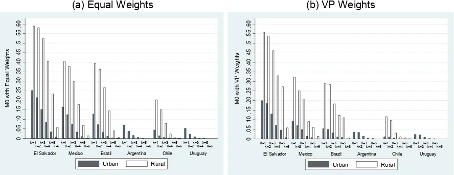
Figure 3: M_{0measure for different} k_{values in 2006}

Urban vs. rural areas

(a) Equal Weights (b) VP Weights

0 .0 5 .1 0 .1 5 .2 0 .2 5 .3 0 .3 5 .4 0 .4 5 .5 .5 5 .6 0 M 0 w it h E q u a l W e ig h ts

El Salvador Mexico Brazil Argentina Chile Uruguay

k=1

k=2k=3k=4k=5k=6k=1k=2k=3k=4k=5k=6k=1k=2k=3k=4k=5k=6k=1k=2k=3k=4k=5k=6k=1k=2k=3k=4k=5k=6k=1k=2k=3k=4k=5k=6

Urban Rural 0 .0 5 .1 0 .1 5 .2 0 .2 5 .3 0 .3 5 .4 0 .4 5 .5 .5 5 .6 0 M 0 w it h V P W e ig h ts

El Salvador Mexico Brazil Argentina Chile Uruguay

k=1

k=2k=3k=4k=5k=6k=1k=2k=3k=4k=5k=6k=1k=2k=3k=4k=5k=6k=1k=2k=3k=4k=5k=6k=1k=2k=3k=4k=5k=6k=1k=2k=3k=4k=5k=6

Urban Rural

Figure 3 presents the most recent estimate of M0using equal weights in (a), and using VP weights in (b).

Whenever possible, urban and rural estimates are presented. Not surprisingly, the rural estimates are at least twice the urban values, in all cases. One particularly important point to note from this figure is that in the urban areas of Argentina, Chile and Uruguay, both with equal and VP weights, the M0 estimate

becomes virtually 0 (less than 5 per cent) with k≥2. This is a consequence of both a small fraction of the population in the urban areas being deprived in two or more dimensions simultaneously and a relatively low average deprivation share among the poor.33_{However, this is not the case for the rural areas of Chile}

and both the urban and rural areas of Brazil, El Salvador and Mexico. For these countries and regions, the M0 estimates become closer to zero only with much higher k values. Note, for example, that in the

rural areas of El Salvador and Mexico, the M₀estimates using equal weights become below 5 per cent only with the intersection approach at the identification step (k=6). This suggests a pattern in terms of coupled versus single deprivations in the analysed countries. In Brazil, Mexico, El Salvador and in the rural areas of Chile, if someone is deprived in one indicator, she is likely to be deprived in several other indicators at the same time, while if she lived in the urban areas of Argentina, Chile or Uruguay, she is likely to be deprived only in that single indicator. Moreover, within Brazil, El Salvador and Mexico, coupled deprivations are more likely in rural areas than in urban ones.

Finally, comparing the two weighting schemes, the M0estimates using the VP weights are smaller than

those using equal weights. This is to be expected, since the requirement to be counted as poor is generally more demanding for a given kthan with equal weighting – unless the person is deprived in the highest weighted dimensions (income and children in school), which is less likely as these are among the lowest deprivation counts.34_{Assuming the participatory study from which these weights were derived is}

representative of the poor in Latin America, the estimates suggest that when dimensions are weighted according to the value ranking the poor assign, multidimensional poverty is lower. They care more about having enough income and their children in school, which have relatively lower deprivation rates, than

33_{Indeed, with equal weights for example, the multidimensional headcount with k=2 in 2006 is 10 per cent in Argentina, 8}

per cent in Chile and 6 per cent in Uruguay, whereas the average deprivation share is about 0.38 in the three countries (2.3 dimensions). This can be verified in panel (a) of figure 2.

34_{For example, when VP weights are used and the cut-off is k=1, someone living in a household deprived either in income or}

having access to sanitation and a household head with five or more year of education, which have relatively higher deprivation rates.

As explained in Section 3 above, the M₀ measure is the product of two informative measures: the multidimensional headcount ratio Hand the average deprivation share across the poor A. The evolution of M0 together with its two components H and Aover the study period is presented in figure 4 for the

case of k=2 and equal weights. Figure 4 panel A refers to rural areas of Brazil, Chile, El Salvador and Mexico, while panel B refers to urban areas of these countries together with Argentina and Uruguay.

k=2 is chosen because it is the minimum k that requires an individual to be deprived in more than one dimension so as to be considered poor (i.e. it is ‘truly’ multidimensional) and at the same time it is meaningful for all countries (for higher k values the aggregate M₀estimate becomes virtually zero in the urban areas of Chile, Argentina and Uruguay).

Figure 4 shows clearly the different patterns of evolution of multidimensional poverty in rural and urban areas of the six countries. Both in the urban and rural areas of Brazil, Chile, El Salvador and Mexico, the reduction in M₀ was the result not only of reductions in the percentage of people deprived in two or more dimensions, but also of the fact that, on average, they became poor in fewer dimensions. However, the proportional reductions in each of the components of M0differed. In both the rural and urban areas

of Chile and Brazil, as well as in the urban areas of Mexico, the reduction in the percentage of the poor was relatively larger than the reduction in the average deprivation, especially in Chile. On the contrary, in both the rural and urban areas of El Salvador the proportional reduction in Awas larger than that of H, while in rural Mexico, both the percentage of the poor and the average deprivation were reduced in similar proportions. In urban Uruguay there was a very small reduction of M0led by a reduction in H;

Figure 4: Evolution Over Time of M0and its Components with k=2 and Equal Weights

Panel A Panel B

Adjusted Headcount Ratio M0

Rural Areas

Adjusted Headcount Ratio M0

Urban Areas 0 .1 0 .2 0 .3 0 .4 0 .5 0 .6 0 .7 0 .8 M 0 w it h k = 2 a n d E q u a l W e ig th s

1992 1995 2000 2003 2006 Year

Rural Brazil Rural Chile Rural El Salvador Rural Mexico

0 0 .1 0 .2 0 .3 M 0 w it h k = 2 a n d E q u a l W e ig th s

1992 1995 2000 2003 2006 Year

Urban Argentina Urban Brazil Urban Chile Urban El Salvador Urban Mexico Urban Uruguay

Multidimensional Headcount Ratio H

Rural Areas

Multidimensional Headcount Ratio H

Urban Areas 0 .2 0 .4 0 .6 0 .8 1 H w it h k = 2 a n d E q u a l W e ig th s

1992 1995 2000 2003 2006 Year

Rural Brazil Rural Chile Rural El Salvador Rural Mexico

0 0 .2 0 .4 0 .6 H w it h k = 2 a n d E q u a l W e ig th s

1992 1995 2000 2003 2006 Year

Urban Argentina Urban Brazil Urban Chile Urban El Salvador Urban Mexico Urban Uruguay

Average Deprivation Share across the poor A

Rural Areas

Average Deprivation Share across the poor A

Urban Areas .4 .5 .6 .7 A w it h k = 2 a n d E q u a l W e ig th s

1992 1995 2000 2003 2006 Year

Rural Brazil Rural Chile Rural El Salvador Rural Mexico

0 .3 0 .4 0 .5 0 .6 A w it h k = 2 a n d E q u a l W e ig th s

1992 1995 2000 2003 2006 Year

Urban Argentina Urban Brazil Urban Chile Urban El Salvador Urban Mexico Urban Uruguay

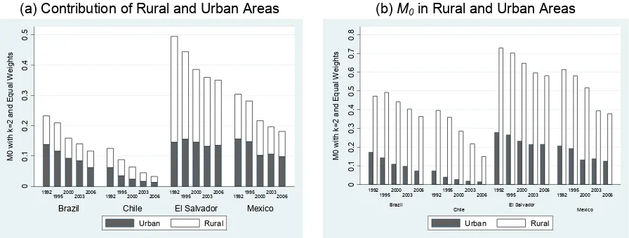
The last figure of this section shows the relative contribution of urban versus rural areas to the aggregate

M₀ estimates using k=2 and equal weights. Panel (a) of figure 5 presents the contribution of each of them to the aggregate M₀estimates. The height of each bar corresponds to the aggregate estimate, and the shaded regions to the relative contributions. To complement this graph, panel (b) presents the actual

In the urban-rural contributions to aggregate poverty, the population weight of urban areas plays a significant role. In Brazil, Chile and Mexico in 1992, although the M₀estimate in rural areas was three or more times that in urban areas, urban poverty accounted for 47 per cent or more of overall poverty because the urban population share was 76 per cent or higher in the three countries. Over the study period, the contribution of urban areas to overall poverty decreased by 8 percentage points in Brazil (to 51 per cent) and by 6 percentage points in Chile (to 41 per cent) because, although the urban population share increased, the poverty reduction achieved in urban areas was larger than that achieved in rural ones. In contrast, the urban contribution to overall poverty increased in Mexico by 4 percentage points: a combination of the increase in the share of urban population and a reduction in multidimensional poverty that was more similar in rural than in urban areas. The only case in which the urban contribution to overall poverty was low (only 28 per cent) in 1992 was El Salvador because multidimensional poverty in rural areas was two an a half times that of urban areas and also because the urban population share was only 52 per cent. Over the period, the contribution of urban areas to aggregate M0 in the country

increased to 37 per cent, given that the share of urban population increased to 63 per cent and the reduction in M₀in rural areas was similar to that in urban areas.

Figure 5: Evolution of Multidimensional Poverty –M0with k=2 and Equal Weights

Rural and Urban Areas, 1992–2006

(a) Contribution of Rural and Urban Areas (b) M0in Rural and Urban Areas

0 0 .1 0 .2 0 .3 0 .4 0 .5 M 0 w it h k = 2 a n d E q u a l W e ig h ts

Brazil Chile El Salvador Mexico

1992

1995200020032006 19921995200020032006 19921995200020032006 19921995200020032006

Urban Rural 0 0 .1 0 .2 0 .3 0 .4 0 .5 0 .6 0 .7 0 .8 M 0 w it h k = 2 a n d E q u a l W e ig h ts Brazil

Chile El Salvador Mexico

1992

1995200020032006 19921995200020032006 19921995200020032006 19921995200020032006

Urban Rural

(c) Evolution of the Urban Population Share Over Time

5 0 5 5 6 0 6 5 7 0 7 5 8 0 8 5 9 0 % o f U rb a n P o p u la ti o n

1992 1995 2000 2003 2006 Year