Evaluating simple metaheuristics for the generalized steiner problem

(1)

Evaluating simple metaheuristics

for the Generalized Steiner Problem

Sergio Nesmachnow

Centro de Cálculo, Instituto de Computación Facultad de Ingeniería, Universidad de la República

Montevideo, 11300, Uruguay.

ABSTRACT

This article presents the empirical evaluation of several simple metaheuristics applied to solve the Generalized Steiner Problem (GSP). This problem models the design of high-reliability communication networks, demanding a variable number of independent paths linking each pair of terminal nodes. GSP solutions are built using intermediate nodes for guaranteeing path redundancy, while trying to minimize the design total cost. The GSP is a NP-hard problem, and few algorithms have been proposed to solve it. In this work, we present the resolution of several GSP instances whose optimal solutions are known, using metaheuristic techniques. The comparative analysis shows promising results for some of the studied techniques. Keywords: metaheuristics, Generalized Steiner Problem, reliable network design.

1 INTRODUCTION

The fast development of network infrastructures, software and Internet services has been driven by the growing demand for data communications over the last twenty years. This is the reason for a renewed interest in network design problems relating to routing information through the net [3,15]. Finding a reliable, fault tolerant connection topology is a capital issue in communication networks design. Since the size of the existing communication networks is continuously enlarging, the underlying instances of related optimization problems frequently pose a challenge to existing algorithms. In consequence, the research community is nowadays searching for new algorithms, able to improve over the traditional ones, whose low efficiency often makes them useless for solving real-life problems of large size in reasonable times. We present the application of several simple metaheuristics for solving problems modeled by the Generalized Steiner Problem. Given a communication network with some distinguished terminal nodes, the GSP consists in designing a minimum cost subnetwork verifying a set of prefixed connection requirements for pairs of terminal nodes. Minimizing the connection costs is in conflict with the reliability maximization of the resulting network. For example, a minimum cost model with no path redundancy would lead to topologies unable to tolerate even a single component failure. The GSP incorporates additional connectivity requirements that real-life situations demand, hence guaranteeing high network reliability. This problem has been scarcely addressed in the past; in previous works, we developed pure and hybrid evolutionary algorithms in the aim of solving it with high numerical accuracy and efficiency [2,12,13]. Since it does not exist a standard GSP test suite, we evaluated our algorithms using randomly generated test instances, whose optimum solutions are unknown. This work presents an empirical evaluation of the results achieved for several simple metaheuristic techniques for solving GSP instances with optimal solutions known.

These test instances were designed replicating small graphs for which its optimal solution can be found using exhaustive methods in moderate execution times.

The article is structured as follows. Next section briefly presents heuristics and metaheuristics techniques. Section 3 describes the GSP and popular variants. The algorithms studied are presented in Section 4 and the implementation details are offered in Section 5. Section 6 presents the test instances generated, just before the discussion on the experiments and results in Section 7. Conclusions and future work are formulated in the last section.

2 HEURISTIC AND METAHEURISTICS

The complexity of known algorithms for solving NP-hard combinatorial optimization problems increases in a super polynomial factor related with the input size. For these problems, the huge time and computational resources they demand limit the applicability of exact algorithms. In this scenario, when using analytical techniques, mathematical programming or exhaustive search methods is impractical, heuristic techniques have emerged as flexible and robust methods. Although they could fail in computing a true optimum for optimization problems, heuristics get appropriate quasi-optimal solutions for problems found in several areas of application. In a higher level of abstraction, metaheuristic techniques propose generic schemata for solving complex problems. These schemata can be instanced for defining specific algorithms, working following the same general features.

In this work, we use population-based metaheuristics (Evolutive Algorithms), trajectory-based metaheuristics (Simulated Annealing and Variable Neighborhood Search), and hybrids algorithms for solving the GSP. The algorithms studied are “simple” metaheuristics, meaning that they do not use specific information related with the problem to solve -except the evaluation of the function to optimize, used for guiding the search-. The search space is explored using fully stochastic mechanisms, defined by random operators for all the algorithms considered.

3 THE GENERALIZED STEINER PROBLEM

3.1 GSP formulation

The GSP formulation considers the following elements: · An undirected graph G = (V,E), where V is the set of

nodes and E is the set of edges representing the bidirectional (full-duplex) communication channels. · A cost matrix C associated to the edges of the graph G. · A fixed subset of the node set T Í V, named terminal

nodes, whose cardinality is nT= |T|, such that 2 £nT£n, where n = |V| is the cardinality of the node set V. · A nT x nT symmetric matrix R = rij, i,j Î T, whose

(2)

Solving the GSP consists in finding a minimum cost subgraph GT ÍG, where any pair of nodes i,jÎT, is rij edge connected in GT. This last means that there must exist

rij disjoint paths, with no single shared edge between terminal nodes i y j en GT. The nodes not belonging to the terminal node set are known as Steiner nodes. No connection requirements are formulated over them, and they can either be included or not in the optimum solution, depending on the convenience of their use.

3.2 Steiner problems, complexity and resolution The GSP complexity is consequence of its general formulation, since the problem allows non-uniform connection requirements between terminal nodes. Some variants of the Steiner problem simplify this requirement. The k–connection problem subclass demand a common number (k) of disjoint paths for every pair of terminal nodes. The simplest case of Steiner problem requires only one single path between terminal nodes. Optimal solutions to this problem exhibit a tree topology, and the problem is thus called the Steiner Tree Problem (STP).

The GSP is on the NP-hard problems class [9]. Even the STP, with the less general path restriction requirement, is NP-complete [10]. As a consequence, the Steiner problem class is not amenable to exact methods as problem instances grow in size. Instead, heuristic methods are usually employed, since they can obtain acceptable or optimal solutions in reasonable execution times.

Several heuristics and metaheuristics techniques have been used for solving the simple variants of Steiner problems (STP and 2–connection problems). However, up to now they have not been proposed for facing the Generalized Steiner Problem. In our working group at Universidad de la República, we designed evolutive algorithms for solving the generalized problem trying to keep the codification and variation operators as simple as possible [2,12,13].

4 ALGORITHMS STUDIED

This section presents the metaheuristics considered in the study: Genetic Algorithms (GA) in its classical formulation and the CHC variant, Simulated Annealing (SA), Variable Neighborhood Search (VNS) y two hybrids combining GA with SA y VNS respectively.

4.1 Genetic Algorithm

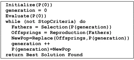
The classical GA formulation is based on the schema for an Evolutionary Algorithm (EA) presented on Figure 1 [4]. EAs are search methods that apply stochastic operators on a pool of individuals (the population) in order to improve their fitness, a measure related to the objective function, which associates a value to individuals indicating their suitability to the problem. Every individual in the population is the encoded version of a tentative solution. Initially, this population is randomly generated.

Iteratively, EAs apply operations like recombination of parts of two individuals and random changes (mutations) in their contents, guided by a selection-of-the-best technique to tentative solutions of higher quality. GA is a particularly popular type of EA, which defines selection, recombination and mutation operators applying them to the population of potential solutions in each generation. In the classical formulation of a GA the ”reproduction” operators include recombination and mutation. GAs have been successfully applied in many real applications of high complexity [4,8]. The GA used in this work is based on previously presented works by the author [2,12,13].

Initialize(P(0)) generation = 0 Evaluate(P(0))

while (not StopCriteria) do

Fathers = Selection(P(generation)) Offsprings = Reproduction(Fathers) NewPop=Replace(Offsprings,P(generation)) generation ++

[image:2.595.310.527.68.166.2]

P(generation)=NewPop return Best Solution Found

Figure 1: Schema for an Evolutionary Algorithm.

4.2 CHC Algorithm

[image:2.595.312.528.394.551.2]

CHC stands for Cross generational elitist selection, Heterogeneous recombination, and Cataclysmic mutation [6]. CHC is a specialization of the classical GA, which uses a conservative selection strategy, perpetuating the k better individuals. In addition, no mutation is applied, and a special recombination operator is introduced: uniform crossover (HUX), which randomly swaps exactly half of the bits that differ between the two parent strings. Parents are randomly selected, but only those that differ from each other by some number of bits are allowed to reproduce (this mating threshold is often set to 1/4 of the chromosome length, and each generation when no offspring is inserted into the new population, the threshold is reduced by 1). CHC introduces diversity by a re-initialization procedure using the best individual found so far as a template for creating a new population after convergence is detected (i.e., when no offspring can be inserted after a number of generations).

Figure 2 presents a schema for CHC algorithm.

Initialize(P(0)) generation = 0

distance = ChromosomeLength/4 Evaluar(P(0))

while (not StopCriteria) do

Fathers = Selection(P(generation)) Offsprings = HUX(Fathers)

Evaluate (Offsprings))

NewPop=Replace(Offsprings,P(generation)) if (NewPop == P(generation)) then

distance -- generation ++

P(generation) = NewPop if (distance == 0) then

Reinitialize(P(generation)) distance = ChromosomeLength/4 return Best Solution Found

Figure 2: Schema for CHC algorithm.

4.3 Simulated Annealing

Simulated Annealing is a local search optimization method based on Metropolis Monte Carlo simulation to find the most stable configuration for an n-body system [11]. SA maintains a current solution for the problem (analogous to the current state of a system) with an associated objective function (analogous to the energy function) for which we want to find its global minimum (analogous to the ground state). SA employs a temperature T to control the probability of accepting worse solutions than the current one. There is no obvious analogy for the temperature T (there is not such a free parameter on the combinatorial optimization problem), and so defining an appropriate “annealing schedule” for avoiding local minima is an art. SA parameters (initial temperature, and number of iterations performed at each step –Markov chain length–) are often determined empirically.

(3)

Initialize(T) step = 0

Sol = InitialSol() Value = Evaluate(Sol) repeat

repeat step ++

NewSol = Generate(Sol,T) // Transition

NewValue = Evaluate(NewSol) if Accept(Value,NewValue,T) Sol = NewSol

Value = NewValue

until ((step mod LengthMarkovChain)==0) T = Update(T)

[image:3.595.72.289.69.225.2]

until (StopCriteria) return Sol

Figure 3: Schema for Simulated Annealing algorithm.

4.4 Variable Neighborhood Search

Variable Neighborhood Search applies a local search defining a systematical neighborhood exploration for finding new solutions [15]. Our VNS algorithm follows a general schema, using two sets of neighborhood structures: one for the random shaking phase, which generates a random solution, and the other one for the local search using a Variable Neighborhood Descendent (VND)

procedure. Figure 4 presents a schema for VNS algorithm. Initialize neighborhood structures Nk, Nj step = 0

Sol = InitialSol() Valor = Evaluate(Sol) repeat

k = 1 repeat

Sol’= Shake(Sol) // Generate sol in Nk NewSol=VND(Sol’,Nj) // Apply VND in Nj

NewValue = Evaluate(NewSol) if NewValue < Value

Sol = NewSol Value = NewValue k = 1

else k ++ until k==k_max until (StopCriteria) return Sol

Figure 4: Schema for VNS algorithm.

4.5 Hybrid algorithms

Hybridization techniques propose including problem dependent knowledge in a general search algorithm [4]. It could be implemented as problem-dependent encoding and/or special operators (strong hybrids) or by combining several algorithms (weak hybrids). In this work, we used this last option, combining the GA evolutive search with the local search proposed by SA and VNS, defining two hybrid algorithms (GA+SA and GA+VNS), incorporating the local search method as an internal operator in the GA.

5 IMPLEMENTATION

5.1 Problem encoding

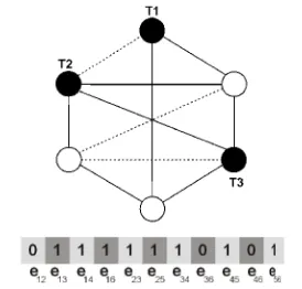
[image:3.595.349.486.70.201.2]

We used an edge-oriented binary representation for encoding GSP solution graphs. A solution is represented as a bit array (indexed from 0 to |E|-1); each bit indicates the presence or absence of a specific edge existing on the original graph. Figure 5 presents an example graph and its encoding using the representation proposed. Terminal nodes are colored dark and labeled T1 to T3 and Steiner nodes are colored white. Present edges on the current solution are drawn with filled lines, while original edges not present on the solution are drawn with dotted lines.

Figure 5: Edge-based binary codification By using such a binary codification, the evolutionary operators (recombination, mutation) are easy to implement. But a difficult must be solved: the operators could work out non-feasible solutions. We worked discarding non-feasible individuals [2, 5, 12, 13]. This decision simplifies the algorithm, avoiding quantifying how far those individuals are from the set of feasible solutions and also avoiding introducing a penalty function for measuring their fitness value. The feasibility check has two components: a simple heuristic discards a solution if the degree of any terminal node is smaller than the maximum connection requirement for this node. When the degrees of all the terminal nodes are compatible with the connection requirements, we use the Ford-Fulkerson algorithm [7] for finding paths between pairs of terminal nodes, considering one of them as the source and the other as the sink. Assuming unitary capacity for each arc, the maximum flow between source and sink matches the maximum number of disjoint paths between the nodes. If this number is smaller than the correspondent connection requirement, then the solution is not feasible.

The population is randomly initialized using a procedure that arbitrarily eliminates up to 5% of the edges from the original graph representation. After that, the feasibility check is applied to discard non-feasible initial solutions. Each non-feasible solution detected is dropped from the initial population and the initialization procedure is applied again to generate another one.

5.2 Optimizing function

The optimizing function evaluates the total cost of the network represented by the solution graph, adding the cost of each edge, as Eq. (1) formulates.

å

-=

= 1

0 ) ( E

i i C

f (1)

5.3 Operators and parameters

The operators and parameters used by the algorithms are: · SA: Transition inverts five edges, proportional decaying

schema for temperature (Tk = a.Tk-1, a = 0.99).

· GA: Proportional selection, two point recombination, bit-flip mutation.

· CHC: HUX crossover, elitist selection, re-initialization based on SA movement, applied until generating a feasible solution.

· VNS: Neighborhood defined by Hamming distance in the binary codification.

[image:3.595.73.285.334.526.2]

(4)

We use a stop criterion of 2000 generations for the EAs, and 10000 iterations for SA and VNS. EAs use a population of 120 individuals, randomly initialized eliminating up to 5% of the edges until obtaining feasible solutions. The probability of recombination is fixed at 0.9 for the GA and the hybrids, and the mutation probability has a value of 0.01. In CHC the reinitialization procedure involves the 35 % of the individuals in the population.

VNS parameters are kmax=3 for the shaking phase, and j=3

i<=>?@ ABC@E?C FB>G Ei<HIJKL

In the hybrid algorithms, the local search operator is applied with probability 0.01 in each generation. GA+SA uses a short Markov chain (length 10) and 20 iterations, for reducing the computational effort of applying SA as an inner operator in the GA.

5.4 The MALLBA library

We implemented the algorithms using MALLBA, a library that provides skeletons for optimization algorithms [1]. The algorithms and its interaction with the problem are implemented by C++ classes that represent an abstraction of the entities participating in the resolution method: · Provided classes implements internal aspects of the

skeleton in a problem-independent way. The most importantprovided classes are Solver (the algorithm) and SetUpParams.

· Required classes specify problem-related information. Each skeleton includes the provided classes Problem and Solution that encapsulate the problem-dependent entities needed by the resolution method.

The MALLBA library is available publicly at http://neo.lcc.uma.es/mallba/easy-mallba.

5.5 Execution platform

The algorithms were executed on an Intel Pentium IV computer at 2.4 GHz having 512 Mb RAM and the SuSE Linux 8.1 operating system.

6 GSP TEST SUITE

The GSP has been scarcely addressed, and therefore there do not exist standardized problem benchmarks or test suites. In previous works, we used a random test instances generator for evaluating the algorithms designed [12,13]. Since we do not know the instances optimum values, a comparative analysis is possible, but we cannot evaluate the distance to the optimum values. In this work, we propose the empirical analysis of the results obtained by

simple metaheuristics for GSP instances with known optimal values. These test instances were designed replicating small graphs whose optimal solutions can be obtained using exhaustive search methods. The replicas have a structure splitted in several connected components, but this fact is indifferent for the algorithms, which do not use problem-dependant operators, thus they consider the replicated graph as a problem with unknown structure. Obviously, these test instances are not realistic scenarios, and they do not formulate the worst case complexity. However, using these optimum-known instances we are able to evaluate the quality of results obtained by the proposed metaheuristics.

Table 1 presents the non replicated graphs details, showing the total number of nodes and terminal nodes, edges, and the connectivity degree (number of edges number of edges in a complete graph). Figures 6, 7, 8 and 9 present the non replicated test instances.

Instance Nodes Terminals Edges Connectivity degree

graph_1 6 4 15 1.000

graph_2 10 2 37 0.561

graph_3 16 6 25 0.077

[image:4.595.308.531.262.330.2]

graph_4 15 5 26 0.248

Table 1: Non replicated graphs details.

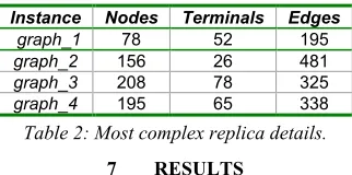
We replicated the instances shown in Table 1 between 2 and 13 times, building more complex instances allowing studying the algorithms efficacy when the problems grow in size. K?=C ils for the most complex replica generated (13

replicas) are shown in Table 2.

[image:4.595.338.499.389.469.2]

Instance Nodes Terminals Edges graph_1 78 52 195 graph_2 156 26 481 graph_3 208 78 325 graph_4 195 65 338

Table 2: Most complex replica details.

7 RESULTS

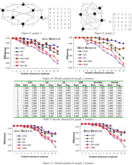
[image:4.595.70.497.578.711.2]

Tables 3, 4, 5 and 6 present the results obtained by the studied algorithms for the GSP instances generated, presenting best and average values of “efficiency” (ratio result/optimum) achieved for each algorithm on 10 independent runs for each replicated graph. Figures 10, 11, 12 and 13 summarize the information, showing graphics for average and best results for each algorithm (we omit best values for the GA+SA algorithm since they do not differ significantly for those obtained by the GA).

Figure 6: graph_1. Figure 7: graph_2.

÷÷ ÷ ÷ ÷

ø ö

çç ç ç ç

è æ

=

0 2 3 4

2 0 2 3

3 2 0 2

4 3 2 0

R

÷÷ ø ö çç è æ =

0 4

4 0 R

(5)

Figure 8: graph_3. Figure 9: graph_4.

0.76 0.80 0.84 0.88 0.92 0.96 1.00

1 2 3 4 5 6 7 8 9 10 11 12 13

Problem dimension (replicas)

E ff ic ie n c y CHC GA SA GA+VNS VNS GA+SA

Figure 10: Results quality for graph_1 instance.

CHC GA SA VNS GA+VNS GA+SA

#rep Best Avg. Best Avg. Best Avg. Best Avg. Best Avg. Best Avg.

1 1.000 1.000 1.000 1.000 1.000 1.000 1.000 1.000 1.000 1.000 1.000 1.000 2 1.000 1.000 1.000 1.000 1.000 0.987 1.000 0.995 1.000 1.000 1.000 1.000 3 1.000 1.000 1.000 1.000 1.000 0.975 1.000 0.977 1.000 1.000 1.000 1.000 4 1.000 1.000 1.000 0.972 0.958 0.956 0.979 0.962 1.000 0.989 1.000 0.977 5 1.000 0.993 0.983 0.961 0.966 0.936 0.983 0.951 1.000 0.968 0.984 0.963 6 1.000 0.987 0.972 0.966 0.958 0.934 0.972 0.961 1.000 0.972 0.973 0.966 7 1.000 0.984 0.964 0.959 0.940 0.923 0.964 0.947 0.988 0.977 0.967 0.953 8 0.989 0.950 0.968 0.931 0.916 0.900 0.937 0.918 0.989 0.958 0.966 0.946 9 0.981 0.947 0.963 0.921 0.898 0.881 0.925 0.903 0.990 0.938 0.964 0.923 10 0.983 0.948 0.933 0.931 0.883 0.874 0.916 0.889 0.950 0.959 0.933 0.929 12 0.977 0.940 0.916 0.906 0.863 0.853 0.878 0.865 0.931 0.922 0.916 0.901 13 0.965 0.946 0.888 0.891 0.833 0.818 0.861 0.856 0.923 0.918 0.923 0.912

[image:5.595.68.510.64.615.2]

Table 3: Results obtained for graph_1 instance.

1 1.000 1.000 1.000 0.998 1.000 0.970 1.000 0.985 1.000 1.000 1.000 1.000 2 1.000 0.999 1.000 0.979 1.000 0.950 1.000 0.977 1.000 0.990 1.000 0.981 3 1.000 0.983 1.000 0.956 0.970 0.920 0.990 0.951 1.000 0.962 1.000 0.965 4 1.000 0.971 0.979 0.945 0.964 0.893 0.979 0.932 0.993 0.953 0.981 0.948 5 1.000 0.961 0.989 0.929 0.960 0.871 0.994 0.894 1.000 0.938 0.983 0.932 6 0.981 0.952 0.957 0.901 0.919 0.850 0.952 0.891 0.962 0.922 0.960 0.921 7 0.976 0.940 0.959 0.874 0.918 0.832 0.931 0.862 0.980 0.914 0.954 0.894 8 0.968 0.928 0.918 0.855 0.893 0.812 0.900 0.839 0.946 0.898 0.920 0.875 9 0.978 0.919 0.879 0.844 0.870 0.793 0.879 0.823 0.914 0.871 0.874 0.863 10 0.937 0.900 0.891 0.821 0.854 0.782 0.886 0.801 0.917 0.859 0.890 0.838 12 0.935 0.890 0.883 0.804 0.836 0.771 0.870 0.790 0.896 0.843 0.885 0.821 13 0.933 0.892 0.902 0.800 0.840 0.754 0.881 0.775 0.919 0.825 0.890 0.812

0.82 0.86 0.90 0.94 0.98

1 2 3 4 5 6 7 8 9 10 11 12 13

E ff ic ie n c y CHC GA SA GA+VNS VNS ÷ ÷ ÷ ÷ ÷ ÷ ø ö ç ç ç ç ç ç è æ = 0 1 1 1 1 1 0 1 2 2 1 1 0 3 3 1 2 3 0 3 1 2 3 3 0 R ÷ ÷ ÷ ÷ ÷ ÷ ÷ ÷ ø ö ç ç ç ç ç ç ç ç è æ = 0 2 3 2 3 2 2 0 2 3 2 3 3 2 0 2 3 2 2 3 2 0 2 3 3 2 3 2 0 2 2 3 2 3 2 0 R

A

VG

.

R

ESULTS

B

EST

R

ESULTS

0.82 0.86 0.90 0.94 0.98

1 2 3 4 5 6 7 8 9 10 11 12 13

E ff ic ie n c y CHC GA SA GA+VNS VNS

A

VG

. R

ESULTS

B

EST

R

ESULTS

0.80 0.84 0.88 0.92 0.96 1.00

1 2 3 4 5 6 7 8 9 10 11 12 13

(6)

[image:6.595.78.517.78.554.2]

1 1.000 1.000 1.000 1.000 1.000 1.000 1.000 1.000 1.000 1.000 1.000 1.000 2 1.000 1.000 1.000 1.000 1.000 0.987 1.000 0.995 1.000 1.000 1.000 1.000 3 1.000 1.000 1.000 1.000 1.000 0.975 1.000 0.977 1.000 1.000 1.000 1.000 4 1.000 1.000 1.000 0.972 0.958 0.956 0.979 0.962 1.000 0.989 1.000 0.977 5 1.000 0.993 0.983 0.961 0.966 0.936 0.983 0.951 1.000 0.968 0.984 0.963 6 1.000 0.987 0.972 0.966 0.958 0.934 0.972 0.961 1.000 0.972 0.973 0.966 7 1.000 0.984 0.964 0.959 0.940 0.923 0.964 0.947 0.988 0.977 0.967 0.953 8 0.989 0.950 0.968 0.931 0.916 0.900 0.937 0.918 0.989 0.958 0.966 0.946 9 0.981 0.947 0.963 0.921 0.898 0.881 0.925 0.903 0.990 0.938 0.964 0.923 10 0.983 0.948 0.933 0.931 0.883 0.874 0.916 0.889 0.950 0.959 0.933 0.929 12 0.977 0.940 0.916 0.906 0.863 0.853 0.878 0.865 0.931 0.922 0.916 0.901 13 0.965 0.946 0.888 0.891 0.833 0.818 0.861 0.856 0.923 0.918 0.923 0.912

0.80 0.84 0.88 0.92 0.96 1.00

1 2 3 4 5 6 7 8 9 10 11 12 13

E

ff

ic

ie

n

c

y

CHC GA SA GA+VNS VNS

#rep #rep Best Avg. Best Avg. Best Avg. Best Avg. Best Avg. Best

[image:6.595.95.505.402.721.2]

1 1.000 1.000 1.000 1.000 1.000 1.000 1.000 1.000 1.000 1.000 1.000 1.000 2 1.000 1.000 1.000 1.000 1.000 0.987 1.000 0.995 1.000 1.000 1.000 1.000 3 1.000 1.000 1.000 1.000 1.000 0.975 1.000 0.977 1.000 1.000 1.000 1.000 4 1.000 1.000 1.000 0.972 0.958 0.956 0.979 0.962 1.000 0.989 1.000 0.977 5 1.000 0.993 0.983 0.961 0.966 0.936 0.983 0.951 1.000 0.968 0.984 0.963 6 1.000 0.987 0.972 0.966 0.958 0.934 0.972 0.961 1.000 0.972 0.973 0.966 7 1.000 0.984 0.964 0.959 0.940 0.923 0.964 0.947 0.988 0.977 0.967 0.953 8 0.989 0.950 0.968 0.931 0.916 0.900 0.937 0.918 0.989 0.958 0.966 0.946 9 0.981 0.947 0.963 0.921 0.898 0.881 0.925 0.903 0.990 0.938 0.964 0.923 10 0.983 0.948 0.933 0.931 0.883 0.874 0.916 0.889 0.950 0.959 0.933 0.929 12 0.977 0.940 0.916 0.906 0.863 0.853 0.878 0.865 0.931 0.922 0.916 0.901 13 0.965 0.946 0.888 0.891 0.833 0.818 0.861 0.856 0.923 0.918 0.923 0.912

Best Avg. Best Avg. Best Avg. Best Avg. Best Avg. Best Avg.

> 0.95 > 0.90 > 0.88 > 0.80 > 0.83 > 0.71 > 0.83 > 0.85 > 0.92 > 0.87 > 0.90 > 0.88

Table 7: Comparative results.

0.70 0.75 0.80 0.85 0.90 0.95 1.00

1 2 3 4 5 6 7 8 9 10 11 12 13

E

ff

ic

ie

n

c

y

CHC GA SA GA+VNS VNS GA+SA

0.80 0.84 0.88 0.92 0.96 1.00

1 2 3 4 5 6 7 8 9 10 11 12 13

E

ff

ic

ie

n

c

y

CHC GA SA GA+VNS VNS

0.80 0.84 0.88 0.92 0.96 1.00

1 2 3 4 5 6 7 8 9 10 11 12 13

E

ff

ic

ie

n

c

y

CHC GA SA GA+VNS VNS GA+SA

B

EST

R

ESULTS

A

VG

.

A

VG

. R

ESULTS

A

VG

. R

ESULTS

(7)

Instance CHC GA SA VNS GA+VNS GA+SA

graph_1 10.0 14.7 3.2 5.9 25.7 21.3

graph_2 15.2 21.9 5.2 9.0 35.7 29.1

graph_3 13.4 19.8 4.5 8.6 32.5 26.6

[image:7.595.159.443.81.129.2]

graph_4 14.7 21.0 4.9 8.8 34.9 28.9 Table 8: Average execution times (minutes).

Population-based techniques show their superiority for solving all GSP instances studied: CHC, GA and the hybrids achieve superior results than VNS and SA. Using simple operators, trajectory-based techniques are less competitive, showing difficulties to manage the GSP complexity. VNS exhaustive search allows achieving better results than SA, which shows the worst results for all instances. Hybridizing GA with VNS or SA helps to improve the results, since the inner operator provides a new source of diversity in the evolutive search.

CHC achieved systematically the best results, surpassed only in specific cases for GA+VNS. This fact confirms previous results [12,13] where CHC showed as the best alternative for solving the GSP, since its special operators define a more diversified, robust and effective search. The best results achieved for all metaheuristics yielded over 80% respect the optimum value for the largest problems studied. CHC always achieved 95% respect the optimum, while GA and the hybrids results were in the range of 90-95%. This results show that even using simple operators, without including problem-dependant information, EAs are able to achieve high-quality results. Even though we solved low complexity instances, which are not representative of real life scenarios, the high quality of results suggests that previously obtained results for randomly generated scenarios are accurate.

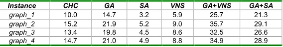
The computational performance was not the main objective of the work, however, we analyzed the execution times for the metaheuristics studied.

Table 8 presents average execution times over 10 independent runs for solving the largest instances studied (13 replicas). Trajectory-based metaheuristics solve the problem quickly since they work with only one solution, while population-based algorithms are between three and four times slower. Hybridization significantly increases the execution times for solving all instances studied.

8 CONCLUSIONS AND FUTURE WORK

This work presents an empirical evaluation of results achieved for several metaheuristic techniques for solving GSP instances with optimal solutions known. The metaheuristics work with the high level of algorithmic simplicity, without incorporating problem-dependant information. Even though we solved non-realistic and medium level complexity instances, the high quality of results achieved promotes previous results obtained for randomly generated and real-life scenarios.

Population-based techniques showed promising results for solving the four GSP instances studied. Using the simple operators proposed, trajectory-based algorithms are less competitive. CHC confirmed previous results obtained for randomly generated instances, achieving the best results, with an error less than 5% for the largest problems. In addition, CHC compute well-suited individuals in a moderately low number of generations. Hybridization techniques improve the results, since they incorporate a new source of diversity in the evolutive search. However, including internal operators significantly increases the execution times.

The study has left two main lines for future work. We shall face theoretical analysis for designing more realistic GSP instances for evaluating the algorithms. On the other hand, several further analysis of the algorithms behavior shall be performed, to study the contribution of advanced operators and hybridization techniques in order to achieve better results. There is room to improve the algorithms to solve larger and more complex GSP instances, for which the current algorithms would need a long time. Related to this point, we are currently working on parallel versions for the algorithms studied, to solve very complex GSP instances by using the computational power of larger clusters of machines.

REFERENCES

[1] E. Alba, C. Cotta. “Optimización en entornos

geográcamente distribuidos. Proyecto MALLBA”,

Congreso Español de Algoritmos Evolutivos y

Bioinspirados, pp. 38–45, 2002.

[2] M. Aroztegui, S. Arraga, S. Nesmachnow, “Resolución del Problema de Steiner Generalizado utilizando un algoritmo genético paralelo”, Congreso Español de Metaheurísticas, Algoritmos Evolutivos y Bioinspirados, pp. 387-394, 2003.

[3] . Corne, M. Oates, G. Smith, Telecommunications

optimization, Wiley, 2000.

[4] L. avis. Handbook of genetic algorithms, Van

Nostrand Reinhold, New York, 1991.

[5] H. Esbensen, “Computing near-optimal solutions to the Steiner problem in a graph using a genetic algorithm”, Networks 26, pp. 173-185, 1995.

[6] L. Eshelman, “The CHC adaptive search algorithm: how to have safe search when engaging in nontraditional genetic recombination”, Foundations of Genetic Algorithms, pp. 265-283, 1991.

[7] L. Ford, . Fulkerson, Flows in Networks. Princeton

University Press, Princeton, 1962.

[8] . Goldberg, Genetic Algorithms in Search,

Optimization and Machine Learning, Addison-Wesley, 1989. [9] V. Kahn, P. Crescenzi, A compendium of NP

optimization problems, online at

http://www.nada.kth.se/theory/problemlist.html

, consulted November 2005.

[10] R. Karp, “Reducibility among combinatorial

problems”, Complexity of Computer Communications, pp. 85-103, 1972.

[11] S. Kirkpatrik, C. Gelatt, M. Vecchi, “Optimization by simulated annealing”, Science, pp. 671–680, 1983.

[12] S. Nesmachnow, H. Cancela, E. Alba. “Técnicas evolutivas aplicadas al diseño de redes de comunicaciones confiables”, Congreso Español de Metaheurísticas, Algoritmos Evolutivos y Bioinspirados, pp. 388-395, 2004. [13] S. Nesmachnow, “Algoritmos genéticos paralelos y su aplicación al diseño de redes de comunicaciones confiables”, Master Thesis, PE Informática, Universidad de la

República, Uruguay, 2004.

[14] W. Pedrycz, A. Vasilakos, Computational intelligence in telecommunications networks, CRC Press, 2001.