Clases características de haces de superficies

(1)

C

_{ENTRO DE}

I

_{NVESTIGACIÓN Y DE}

E

_STUDIOS

A

_{VANZADOS DEL}

I.P.N.

Unidad Zacatenco

Departamento de Matem´aticas

Clases Caracter´

ısticas de

Haces de Superficies

Tesis que presenta

Juan Carlos C

ASTRO

C

ONTRERAS

Para obtener el grado de

Maestro en Ciencias

en la especialidad de Matemáticas

Director de la Tesis

Miguel Alejandro X

ICOTÉNCATL

M

ERINO

(2)

(3)

C

_{ENTER FOR}

R

_{ESEARCH AND}

A

_DVANCED

S

_{TUDIES OF THE}

I.P.N.

Zacatenco Campus

Departament of Mathematics

Characteristic Classes of

Surface Bundles

A dissertation submitted by

Juan Carlos C

ASTRO

C

ONTRERAS

To obtain the degree of

Master of Science in Mathematics

Advisor

Miguel Alejandro X

ICOTÉNCATL

M

ERINO

(4)

(5)

Introduction

Surface bundles are a natural generalization of vector bundles. In this theory as in the

theory of vector bundles characteristic classes of surface bundles provide a powerful tool to

measure how nontrivial a given surface bundle is. Surface bundles are, roughly speaking,

differentiable fiber bundles with fiber a closed orientable surface. Characteristic classes

of surface bundles are elements of cohomology group of classifying space of

orientation-preserving diffeomorphism group of a surface. In the case when the genus of surface

is higher than one the cohomology of such a space turns out to be the same as the

cohomology of mapping class group of surface; in fact, there exist classes called

Munford-Morita-Miller classes that were used by Madsen and Weiss to give a characterization of

the rational cohomology group of stable mapping class group in terms of these classes [18].

If the genus of surface is equal to one, the cohomology of classifying space of

orientation-preserving diffeomorphism group of torus is related to space of automorphic forms using

the Eichler–Shimura isomorphism [12].

These notes follow the work which was worked out in the late 80’s by Shigeyuki Morita

[25, 26, 27]. We study the definition, existence of characteristic classes of surface bundles

and do some explicit calculations.

In the first chapter we introduce the definition of characteristic classes of a surface

bundle and its classification according to the surface used as fiber, namely S2_, _T2 _{or Σ}

g,

the 2-dimensional sphere, the torus or a surface of higher genus, respectively. We argue

why we only study the case when the fiber is either a torus or a surface of higher genus.

In the second chapter we talk about the torus bundles, we give the dimensions of the

rational cohomology groups of the classifying space of orientation-preserving

diffeomor-phism group of T2 _{and provide an example of non-trivial characteristic class of a torus}

bundle.

In the last chapter we define certain characteristic classes of a Σg-bundle, that is, the

Miller-Morita-Mumford classes, and prove the non-triviality of the first characteristic class

of a Σg-bundle.

(10)

(11)

1

Surface Bundles

In this chapter we define the notion of surface bundle, and we give the motivation to

define the characteristic classes of such surface bundles.

1.1 Characteristic classes of differentiable fiber bundles

In this section we give the motivation and the definition of characteristic classes for

dif-ferentiable fiber bundles.

Definition LetF be aC∞_{manifold. An}_F_-_bundle_{is a differentiable fiber bundle whose}

fibers are diffeomorphic toF.

Here DiffF, the diffeomorphism group of F equipped with the C∞ _{topology, is the}

structure group of such bundles. It is interesting in its own right, it also has a relationship

with K-theory but here it is related to the fundamental problem of determine the set of all isomorphism classes ofF-bundles

π :E _−→M

over a given manifold M. It is well-known ([21] or [16] chapter 4 sect. 11–13) that if BDiffF denotes its classifying space, then there is a natural bijection:

{isomorphism classes of F-bundles over M_{} ∼}= [M,BDiffF]

where the right hand side stands for the set of homotopy classes of continuous mappings

(12)

Example Suppose thatM is the n-dimensional sphere Sn_{, we have canonical}

identifica-tions ([31], Corollary 18.6)

[Sn,BDiffF]∼=πn(BDiffF)/π1(BDiffF)

∼

=πn−1(DiffF)/π0(DiffF).

Here the quotient is under the action ofπ1(BDiffF) which is by conjugation. So that we

need to know the homotopy groups of BDiffF or DiffF. It becomes almost impossible to compute these groups for a general manifold F, for example in the case when n = 1, [S1_,_BDiff_F_{] can be identified with the set of all conjugancy classes of} _π

0(DiffF) which is

the group of path components of DiffF. Unfortunately, however, it is almost impossible to compute these groups for a general manifold F. The problem to determine the set [M,BDiffF] should be even more difficult.

In such a situation, it is natural to seek methods of determining whether two given

F-bundles (over the same manifold) are isomorphic to each other o not. One such method is obtained by applying characteristics classes of F-bundles.

Definition Let A be an abelian group and let k be a nonnegative integer. Suppose that, to any F-bundle π : E _−→ M, there is associated a certain cohomology class

α(π) _∈ Hk₍_M_;_A_{) of the base space in such a way that it is natural with respect to any}

bundle map. Then we say thatα(π) is a characteristic class of F-bundles of degree

k with coefficients in A. Here by natural we mean that for any bundle map

E1

f

/

π1

E2

π2

M1 _f //M2

between two F-bundles πi :Ei −→Mi withi= 1,2, we have the equality

(13)

In the terminology of the classifying space, we can write α _∈ Hk_(BDiff_F_;_A_{) and if}

f : X _−→ BDiffF is the classifying map of the given bundle π : E _−→ M, then we haveα(π) =f∗₍_α_{). Namely characteristic classes of} _F_{-bundles are nothing but elements}

of cohomology group of BDiffF. It follows immediately from the definition that two

F-bundles over the same base space which have a different characteristic class are not isomorphic to each other. Thus it is desirable to define as many characteristic classes as

possible.

1.2 Surface bundles

In this section we define what a surface bundle is, we also give the concept of tangent

bundle along the fiber which is going to be useful to define characteristic classes of a

surface bundle. Finally we rewrite the main problem stated before in terms of surface

bundles.

A 2-dimensional C∞ _{manifold, which is compact, connected and without boundary,}

will simply be called a closed surface. The classifying of closed surfaces was done already

in the beginning of twentieth century. As it is well know, the Euler characteristic together

with the property of being orientable or not can serve as a complete set of invariants.

In particular, the set of the diffeomorphism classes of closed orientable surfaces can be

described by the series:

S2, T2, Σg (g = 2,3,· · ·).

HereS2_and_T2 _{denote the 2-dimensional sphere and torus, respectively, and Σ}

g stands for

a closed orientable surface of genus g. Of course we have Σ0 =S2, Σ1 =T2. Henceforth

we assume that an orientation is fixed on each Σg.

Definition A differentiable fiber bundle with fiber Σg is called a surface bundle or a

Σg-bundle.

Let π : E _−→ M be a Σg-bundle. Then the set of all tangent vectors on the total

spaceE which are tangent to the fibers, namely the set:

(14)

becomes a 2-dimensional vector bundle over E. We call ξ the tangent bundle along the fiber of the given Σg-bundle. Sometimes the notation T π will also be used for ξ.

This concept is defined not only for surface bundles but also for general fiber bundles.

Definition A surface bundle π : E _−→ M is said to be orientable if its tangent bundle along the fiber T π is orientable. If a specific orientation is given on T π, then it is called an oriented surface bundle.

Henceforth in this work, all surface bundles are assumed to be oriented and all bundle

maps between them are assumed to preserve the orientation on each fiber.

Definition Two Σg-bundle πi : Ei −→ M with i = 1,2 over the same manifold M are

said to be isomorphic if there exist a diffeomorphismfe:E1 →E2 such that the following

diagram

E1

f

/

π1

E2

π2

M M

commutes andfepreserves the orientation on each fiber.

Our main problem can now be stated as follows:

Determine the set of isomorphism classes of

Σg-bundles over a given manifold.

Let Diff+Σg denote the group of all the orientation preserving diffeomorphisms of Σg

equipped with the C∞ _{topology. It serves as the structure group of oriented Σ}

(15)

1.3 Mapping class group of surfaces

Next we introduce the mapping class group of a surface. It is connected with many areas

in mathematics. Here, for instance, is related to the cohomology groups of classifying

space of structural group of the surface bundles as it is pointed out in Section 1.4.

Let F be a C∞ _{manifold and let Diff}_F _{be its diffeomorphism group. The group of}

path components of DiffF, namely

π0(DiffF),

is called thediffeotopy groupof F. In this work, we denote this group by _D(F). If we write Diff0F for the identity component of DiffF, then we have

D(F) = DiffF/Diff0F.

We can also define this group as follows:

Definition Two diffeomorphismϕ, ψ_∈DiffF of aC∞_manifold_F _{are said to be}_isotopic

to each other if there exist aC∞ _mapping

Φ :F _×[0,1]_−→F

such that Φ(₋,t) : F _{× {}t_{} −→} F is a diffeormorphism for any t _∈ [0,1] and Φ(₋,0) =

ϕ,Φ(₋,1) = ψ.

It can be shown that this notion of isotopy is an equivalence relation. In fact, two

dif-feomorphisms are isotopic if and only if they belong to the same connected component of

DiffF. Hence we can say that_D(F) is the group of all isotopy classes of diffeomorphisms ofF. It follows that in the case of bundles overM =S1_{, we have a natural identification:}

{isomorphism classes of F-bundles overS1_}

∼

={conjugacy classes of _D(F)_}.

Now we restrict to the case when F is a closed orientable surface Σg and consider only

(16)

consider the orientation preserving diffeotopy group of Σg, D+(Σg), also known as the mapping class group _Mg of Σg.

As it will be mentioned later in the last chapter, the mapping class group _Mg plays

an important role also in the Teichm¨uller theory regarding complex structures on Σg. For

this reason,_Mg is also called the Teichm¨uller modular group.

It is clear from the definition that isotopy is a much stronger condition than homotopy.

However, in the case of two-dimensional manifolds, it is classically known that they are

equivalent. Hence we can say that _Mg is the group of all homotopy classes of

orienta-tion preserving diffeomorphism of Σg. Moreover it is also known that Mg is canonically

isomorphic to the group of all homotopy classes of orientation preserving homotopy

equiv-alences of Σg. In fact, since the time of Nielsen, who flourished in the first half of the

twentieth century, it has been known that there exist a natural isomorphism:

Mg ∼= Out+π1(Σg) = Aut+π1(Σg)/Innπ1(Σg).

Here Aut+π1(Σg) denotes the normal subgroup of the automorphism group ofπ1(Σg), with

index two, consisting of those elements which act onH2(Σg;Z) = H2(π1(Σg);Z) trivially,

and Innπ1(Σg) denotes the normal subgroup of all the inner automorphism.

We refer the reader to the book [4] for basic facts about the mapping class group.

1.4 Classification of surface bundles

In this section we overview what we are going to carry out, in a thorough way, in the next

two chapters.

In the case where g = 0, namely for the sphere, it was proved by Smale [29] that the natural inclusion

SO(3) _⊂Diff+S2

is a homotopy equivalence. It follows from this fact that anyS2_{-bundle is isomorphic to the}

sphere bundle of some uniquely defined 3-dimensional oriented vector bundle. Hence the

(17)

oriented vector bundles overM. Since the homotopy type of the classifying spaceBSO(3) is known [23], we may say that this problem is solved.

♠

Next we consider the case g = 1, namely surface bundle whose fibers are diffeomorphic to the torus T2_{. If we identify} _T2 _with _R2_/_Z2_{, then} _T2 _{acts on itself by diffeomorphism}

(which just are translations.) Hence T2 _{can be naturally considered as a subgroup of}

Diff0T2 which is the indentity component of DiffT2. Moreover it is known by Earle-Ells

[10] that the inclusion

T2 _⊂Diff0T2

is a homotopy equivalence. On the other hand, we have an isomorphism

Diff+T2/Diff0T2 =M1 ∼=SL(2;Z).

Passing to classifying space we obtain a fibration

BT2 _−→BDiff+T2 −→BSL(2;Z)

(see [24], Proposition 8.1 & Theorem 11.4.) Notice that BSL(2;Z) is an Eilenberg-MacLane space K(SL(2;Z),1), and thus the cohomology of BSL(2;Z) is that of the discrete group SL(2;Z). The structure of the group SL(2;Z) is classically well known, and we have a homotopy equivalence BT2 ∼₌ _CP∞

×CP∞ (it is because ES1 _×_ES1 _is

contractible space with free action S1 _×_S1_{, the quotient by this action is} _BS1_×_BS1 _so

B(T2_{) =}_B₍_S1_×_S1₎∼₌_BS1_×_BS1_{, therefore} _BT2 ∼₌_CP∞

×CP∞.) Based on these facts we can compute the cohomology of BDiff+T2 which serve as the characteristic classes of

T2_{-bundles. More about this is going to be developed in the second chapter.}

♠

In the case whereg _≥2, the situation changes drastically. More precisely, Earle and Eells proved in [11] Theorem 1.c, that Diff0Σg is contractible so that

BDiff+Σg =K(Mg,1).

(18)

Proposition 1.1 Let g _≥2. Then for anyC∞ _manifold _M_{, we have a natural bijection:}

{isomorphism class of Σg-bundle over M}

∼₌_{conjugacy class of homomorphism π1(M)−→ Mg}

(see [13] lemma 1.19.) In particular if M is simply connected, then any Σg-bundle over

it is trivial since π1(M) = 0 and the constant homomorphism to the identity would be

the only one, therefore just one class of isomorphisms of Σg-bundle would be, in fact, it is

going to be the class of the trivial bundle. However in general, it is almost impossible to

determine the set of all conjugacy classes of homomorphism from a given group to_Mg. It

may be better to understand the above proposition as starting point for the construction

of a classification theory rather than a direct role.

Now let α be a characteristic class of Σg-bundle of degreek with coefficients in a abelian

groupA. Then we can write

α_∈Hk_{(BDiff Σ}

g;A) = Hk(K(Mg,1);A) =:Hk(Mg;A)

(19)

2

Characteristic Classes of

Torus Bundles

In this chapter we study the problem to determine the non-triviality of characteristic

classes of differentiable fiber bundles whose fibers are diffeomorphic to the 2-dimensional

torus T2_{, that is, the problem to compute the cohomology group} _H∗_(BDiff

+T2). More

precisely, we determineH∗_(BDiff

+T2;R) for R=Q orZp with p6= 2,3.

2.1 Introduction

Let Diff0T2 be the connected component of the identity of Diff+T2. Then as is

well-known the factor group Diff+T2/Diff0T2, which is the mapping class group of T2, can

be naturally identified withSL(2;Z). Therefore we have a fibration

BDiff0T2 −→BDiff+T2 −→K(SL(2;Z),1). (2.1)

T2 _{acts on itself by “translations” (viewed} _T2 ₌ _R2_/_Z2_{) and hence it can be considered}

as subgroup of Diff0T2. We see that the action by conjugation of SL(2;Z) on this group

T2 _⊂ _Diff

0T2 is the same as the standard one. Earle and Eells (see [10], Corollary 7.G)

proved that the inclusion T2 _⊂_Diff

0T2 is a homotopy equivalence so that BDiff0T2 has

the homotopy type of BT2 _≃_B_S1_×_B_S1 _≃_CP∞

×CP∞. If we choose suitable elements

x,y _∈H2_(BDiff

0T2;Z), we can write

H∗_(BDiff

(20)

on which SL(2;Z) acts through the automorphism of it given by γ _→ t_γ−1_{, where} _γ _∈

SL(2;Z).

Now let _{Es,t

r ,dr} be the Serre spectral sequence for cohomology (with coefficients in

a commutative ring R) of the fibration 2.1. Then by the above argument, the E2-term is

given by

∞

M

t=0

E₂s,t =Hs(SL(2;Z);R[x,y]) _⇒ H∗(BDiff+T2).

SinceSL(2;Z) =_hα,β _| α4 ₌_α2_β−3 _{= 1}_i₌_Z

4∗Z2 Z6 (see [28], I.4) where

α=

   0 1

−1 0

 

 and β =

   0 1

−1 1

  

therefore the abelianizationH1(SL(2;Z)) ofSL(2;Z) is a cyclic group of order 12 and the

kernel of the natural surjection SL(2;Z)_→H1(SL(2;Z)) is the commutator subgroup of

SL(2,Z), which in turn is isomorphic to a free group of rank 2 (see [5], Exercise 8 in II.4). Moreover the composition of the restriction map with the transfer map

H∗₍_SL_(2;_Z₎₎

×12

(

res

/

/_H∗₍_F₂₎ tr //_H∗₍_SL_(2;Z))

is multiplication by 12 (see [1], Chapter II.5.) Hence applying an argument of group

cohomology (see [6], Proposition III.10.1), we obtain

Proposition 2.1 If s_≥2, then

∞

M

t=0

E₂s,t =Hs(SL(2;Z);R[x,y]) is annihilated by 12. In particular if R=Q or Zn with (n,12) = 1, then

∞

M

t=0

E2s,t =Hs(SL(2;Z);R[x,y]) = 0 for s≥2.

Corollary 2.2 Let k =Q or Zp (p is a prime different from 2 and 3). Then

Hn_(BDiff

(21)

2.2 The action of

SL

(2;

Z

)

on cohomology of the fiber

As is well-knownSL(2;Z) has the following presentation (see [28])

SL(2;Z) = _hα,β _|α4 =α2β−3 = 1_i.

Here, for the convenience of later computations, we choose two generatorsα =

   0 1

−1 0

  

and β =

   0 1

−1 1

 

. The action of SL(2;Z) on H∗_(BDiff

0T2;Z) = Z[x,y] is given by

α(x) =₋y, α(y) =x

β(x) = x₋y, β(y) = x

becauset_α−1 ₌_α _and t_β−1 ₌

   1 1

−1 0

  .

Now for each q _∈ N, let Lq be the submodule of Z[x,y] consisting of homogeneous

elements of degree 2q. Equivalently,Lqis the 2q-th cohomology groupH2q(BDiff0T2;Z) =

H2q_(B_T2_;_Z_{). We choose a basis} _{_xq_,xq−1_y,_{· · ·} _,xyq−1_,yq

} for Lq and let

Aq, Bq ∈SL(q+ 1;Z)

be the matrix representations of the actions of α and β on Lq with respect to the above

basis. Observe that

Aq = (a

(q)

i,j) =              

0 0 _{· · ·} 0 (₋1)q

0 0 _{· · ·} (₋1)q−1 ₀

... ... ... ...

0 ₋1 _{· · ·} 0 0

1 0 _{· · ·} 0 0

(22)

and

Bq = (b( q) i,j)              

1 1 _{· · ·} 1 1

−q ₋(q₋1) _{· · · −}1 0

... ... ... ...

(₋1)q+1_q ₍₋₁₎q+1 _{· · ·} ₀ ₀

(₋1)q+2 ₀ _{· · ·} ₀ ₀

             

are given by

a(_i,jq)=δij :=     

(₋1)q+1−i _j ₌_q_{+ 2}

−i,

0 otherwise

(i,j = 1,_{· · ·} ,q+ 1).

b(_i,jq) = (₋1)i+1

q₋j+ 1

i₋1

where s t

= 0 if t > s (i,j = 1,_{· · ·} , q+ 1).

In the following section we study some basic properties of the matrices Aq and Bq,

their modpreduction and rationalization. In particular we begin computing their minimal polynomials. We will use these facts in Section 2.4 to compute H0₍_SL_(2;_Z_);_L

q(p)) and

H1₍_SL_(2;_Z_);_L

q(p)) with rational and mod p coefficients. Then we will assemble all this

information to getH∗_(BDiff

+T2;Q) andH∗(BDiff+T2;Zp) forp6= 2,3.

2.3 Some technical lemmas

Let p denotes either a prime or 0. We write Aq(p) and Bq(p) for the corresponding

elements ofSL(q+ 1,Zp) ifp is a prime or of SL(q+ 1;Q) ifp= 0. It is easy to prove Lemma 2.3 1. If q is odd, then A2

q = Bq3 = −I. Moreover the minimal polynomials

of Aq and Bq are t2+ 1 and t3+ 1 respectively.

2. If q is even, then A2

q =Bq3 =I and the minimal polynomials of Aq andBq aret2−1

(23)

Corollary 2.4 If q is odd, then both of Aq(p) +I and Bq(p)−I are invertible provided

p₆= 2. In fact we have

(Aq(p) +I)−1 =−

1

2(Aq(p)−I) and

(Bq(p)−I)−1 =−

1 2(B

2

q(p) +Bq(p) +I).

Now let Lq(p) be either Lq ⊗Zp if p is a prime or Lq ⊗Q if p= 0. Aq(p) and Bq(p)

act onLq(p). We assume q is even and define

L−

q(p) ={u∈Lq(p)|Aq(p)u=−u})

L′

q(p) ={u∈Lq(p)|(Bq2(p) +Bq(p) +I)u= 0}.

Lemma 2.5 If p₆= 2 and q= 2r, then

dimL−q(p) =     

r+ 1 r: odd

r r : even

Proof. It is easy to see that

{xq₋yq,xq−1y+xyq−1,xq−2y2₋x2yq−2,_{· · ·} ,xr+1yr−1₋xr−1yr+1,xryr_} r : odd

or

{xq₋yq,xq−1y+xyq−1,xq−2y2₋x2yq−2,_{· · ·} ,xr+1yr−1+xr−1yr+1_} r : even

forms a basis of L−

q(p).

Next we determine dimL′

q. We first consider the casep= 0.

(24)

Proof. Observe that Bq = (b( q)

ij ), where

b(_i,jq) = (₋1)i+1

q₋j+ 1

i₋1

(i,j = 1,_{· · ·}, q+ 1).

(Here we understand that s_t= 0 if t > s). In other words the j-th column ofBq consist

of coefficients of the polynomial (1₋t)q−j+1_.

(1₋t)5 ₍₁₋_t₎4 ₍₁₋_t₎3 ₍₁₋_t₎2 ₍₁₋_t₎ ₍₁₋_t₎0

· · · 1

+ ' ' 1 + ' ' 1 + ' ' 1 + ' ' 1 + ' ' 1

· · · −5 ₋4

+ ' ' −3 + ' ' −2 + ' ' −1 + ' '

0 = TraceB1

· · · 10 6 3

+ ' ' 1 + ' ' 0 + ' '

0 = TraceB2

· · · −10 ₋4 ₋1 0

+ ' ' 0 + ' '

0 = TraceB3

· · · 5 1 0 0 0

+

'

0 = TraceB4

· · · −1 0 0 0 0 0 = TraceB5

... ... ... ... ... ...

Bq is naturally a minor matrix of Bq+1 and if we multiply (1−t)q−j+1 bytq−j+1, we find

out that

TraceBq = the coefficient oftq in the power series

1 +t(1₋t) +t2₍₁₋_t₎2₊_{· · ·}

But we have

∞

X

n=0

(t(1₋t))n = 1 1₋t+t2

= 1

(t₋ω)(t₋ω)

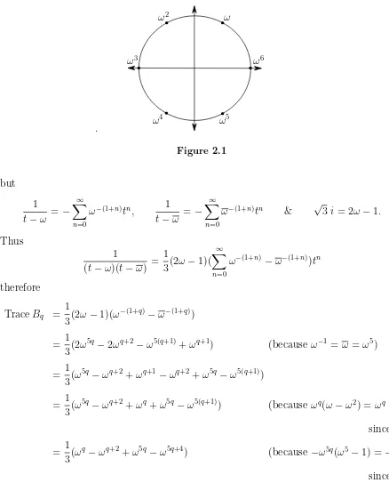
whereω = exp(2πi/6) = 1 2 +

√

3 2 i. Note that 1 ω₋ω =− √ 3 3 i so 1

(t₋ω)(t₋ω) =−

√

3 3 i·

1

t₋ω + √

3 3 i·

1

(25)

ω ω2

ω3

ω4 _ω5

ω6

[image:25.612.86.524.73.616.2]

.

Figure 2.1

but

1

t₋ω =−

∞

X

n=0

ω−(1+n)_tn_, 1

t₋ω =−

∞

X

n=0

ω−(1+n)_tn _& √₃_i_{= 2}_ω

−1.

Thus

1

(t₋ω)(t₋ω) = 1

3(2ω−1)(

∞

X

n=0

ω−(1+n)₋ω−(1+n))tn

therefore

TraceBq =

1

3(2ω−1)(ω

−(1+q)

−ω−(1+q))

= 1 3(2ω

5q

−2ωq+2

−ω5(q+1)₊_ωq+1₎ _(because _ω−1 ₌_ω ₌_ω5₎

= 1 3(ω

5q

−ωq+2₊_ωq+1

−ωq+2₊_ω5q

−ω5(q+1)₎

= 1 3(ω

5q

−ωq+2+ωq+ω5q₋ω5(q+1)) (because ωq₍_ω

−ω2_{) =} _ωq

since ω₋ω2 _{= 1)}

= 1 3(ω

q

−ωq+2₊_ω5q

−ω5q+4₎ _(because

−ω5q₍_ω5₋_{1) =}₋_ω5q+4

since ω5₋_{1 =}_ω4_.)

Then the desired result follows from a direct computation.

Lemma 2.7 If q is even, then

(26)

Proof. According to Lemma 2.3 (ii), the characteristic polynomial of Bq is

(t₋1)a(t2+t+ 1)b

for somea,b_∈N. MoreoverLq = Ker(Bq−I)⊕Ker(Bq2+Bq+I), where dim Ker(Bq−I) = a

and dim Ker(B2

q +Bq+I) = 2b. Because the degree of characteristic polynomial of Bq is

q+ 1 and

(t₋1)a₍_t2₊_t_{+ 1)}b _{= (}_ta

−ata−1₊ (a−1)a

2 t

a−2₊

· · ·) t2b +bt2b−1+bt2b−2+_{· · ·}

=ta+2b_{+ (}_b

−a)ta+2b−1₊_{· · ·}

we obtain

a+ 2b =q+ 1 and a₋b= TraceBq.

but by Lemma 2.6, TraceBq= 1,0,−1 as q = 6k,6k+ 2 or 6k+ 4 respectively.

A simple computation implies the result.

Next we show that the above lemma also holds even if we replace Bq by Bq(p) for

p₆= 3.

Lemma 2.8 Let Bq = (b( q)

ij ) and define Cq = (c( q)

ij ) by

c(ijq) =b

(q)

q+2−i,q+2−j.

Then we haveCq =Bq−1. In other words,Bq andBq−1 are mutually symmetric with respect

to the “center” of them.

Proof. We use induction on q. If q = 1, then

B1C1 =

   1 1

−1 0

  

  0 −1

1 1

  =I.

We assume that BiCi =I for i= 1,· · · ,q−1. Now let b( q)

i be the i-th row of Bq and let

c(jq) be the j-th column of Cq. We can write

Bq =  

 ∗ Bq−1

(₋1)q ₀  

, Cq =        0

c(qq+1)

Cq−1

(27)

Hence by the induction assumption, it sufficies to prove

b(iq)c

(q)

q+1 =δi,q+1

fori= 1,_{· · ·} , q+ 1. Now

i X

k=1

b(_kjq) =

i X

k=1

(₋1)k+1

q₋j+ 1

k₋1

=

q₋j + 1 0 + i X k=2

(₋1)k+1

q₋j k₋2

+

q₋j k₋1

= (₋1)i+1

q₋j i₋1

=b(i,jq)+1 =b (q−1)

ij

for any i,j wherej _≤q. Hence we have

b₁(q)+b(₂q)+_{· · ·}+b(_iq) = (b_i(₁q−1) b_i(₂q−1) _{· · ·} b(_iqq−1) 1)

= (b(_iq−1) 1) (i= 1,_{· · ·} , q) and

b(₁q)+b(₂q)+_{· · ·}+b(_qq₊₁) = ((₋1)q q−1

q

(₋1)q q−2

q

· · · (₋1)q 0

q

1)

= (0 1).

From this we can deduce

b_i(q)= (b(_iq−1) 1)₋(b_i(q₋−₁1) 1) (i= 2,_{· · ·} , q).

Also we have

i X

k=1

c(_k,qq)₊₁=

i X

k=1

b(_qq₊₂) ₋_k,₁

=

i X

k=1

(₋1)q+3−k

q q+ 1₋k

= (₋1)q+2

q q + i X k=2

(₋1)q+3−k

q₋1

q₋k

+

q₋1

q+ 1₋k

= (₋1)q+3−1

q₋1

q₋i

= ₋b(qq−)i+1,2 =−c (q)

i+1,q =−c

(q−1)

(28)

so

i−1

X

k=1

c_k,q(q)₊₁+c_i,q(q)₊₁ = ₋c(_iqq−1)

−c(iqq)+c

(q)

i,q+1 =

thus we obtain

c(_qq₊₁) =c(q)

q −   c

(q−1)

q

0

  .

Now it is easy to see that

b(₁q)c(_qq₊₁) =

q+1

X

k=1

ck,q+1

=

q+1

X

k=1

b(_kq₁) = (₋1)q

q₋1

q

= 0

and b(_qq₊₁) c(_qq₊₁) = 1.

On the other hand if 2_≤i_≤q, then

b(iq)c

(q)

q+1 =b (q)

i

c(qq)− c

(q−1) q

0

=₋b(_iq) c(qq−1)

0

= ((b(iq−−11) 1)−(b (q−1)

i 1)) c(qq−1)

0

= 0

by the induction assumption (the second equality follows from the fact that b(_iq)c(qq) =

b(iq−1)c

(q−1)

q ). This completes the proof.

Lemma 2.9 For eachq let Bq,s(r) where 1≤r ≤q+ 1 and1≤s≤q+ 2−r be the matrix

defined by

B(r)

q,s =       

b(₁q)s b

(q)

1 s+1 · · · b (q) 1 s+r−1

... ...

b(r sq) b(r sq)+1 · · · b (q)

r s+r−1

       .

(29)

Proof. First observe that Bq,s(r) = B_q(r₋)_s₊₁_,₁. Hence we may assume that s = 1 and we

simply write Bq(r) instead of B_q,(r₁). If r = q+ 1, then detB_qq+1 = detBq = 1. So assume

that r < q+ 1. As in the proof of Lemma 2.8 we have

i X

k=1

b(_kjq)=b(_ijq−1)

for any i,j where j _≤q. Hence if we define B(qr) to be the matrix obtained from B

(r)

q by

the following rule:

the i-th row of B(qr) = i X

k=1

(the k-th row of B(r)

q ),

then we have

B(qr)=B

(r)

q−1

and clearly detBq(r) = detB

(r)

q = detB

(r)

q−1. Hence inductively we have

detB(r)

q = detB

(r)

q−1 =· · ·= detB (r)

r−1 = detBr−1 = 1.

This completes the proof.

Lemma 2.10 Assume that q is even and p₆= 3. Then we have

rank(B_q2(p) +Bq(p) +I) = 2k+ 1 if q = 6k,6k+ 2 or 6k+ 4.

Proof. Clearly we have

rank(B2q(p) +Bq(p) +I)≤rank(B2q +Bq+I).

Hence, in view of Lemma 2.7 we have only to show the existence of a minor of (B2

q+Bq+I)

of size (2k+ 1)_×(2k+ 1) (for q= 6k,6k+ 2 or 6k+ 4), whose determinant is a power of 3. Now observe that if i+j > q+ 2, then

b(ijq)= 0.

We are assuming thatq is even so thatB2

q =Bq−1 (see Lemma 2.3 (ii)). Hence by Lemma

2.8, if i+j < q+ 2, then

(30)

Therefore the (i,j)-component of B2

q+Bq+I coincides with that ofBq if (i,j) belongs to

the set

K =_{(i,j)_|i+j < q+ 2 andj > i_}.

If q = 6k+ 2 or 6k + 4, then the minor matrix B_q,(2₂k_k+1)₊₂ of Bq is completely contained in

the region ofBq corresponding to K

b11 b12 · · · b1,2k+2 b1,2k+3 · · · b1,4k+2 · · · b1q b1,q+1

b21 b22 · · · b2,2k+2 b2,2k+3 · · · b2,4k+2 · · · b2q b2,q+1

... ... ... ... ... ... ...

b2k,1 b2k,2 · · · b2k,2k+2 b2k,2k+3 · · · b2k,4k+2 · · · b2k,q b2k,q+1

b2k+1,1 b2k+1,2 · · · b2k+1,2k+2 b2k+1,2k+3 · · · b2k+1,4k+2 · · · b2k+1,q b2k+1,q+1

... ... ... ...

bq+1,1 bq+1,2 · · · bq+1,q bq+1,q+1

                                 

so thatB_q,(2₂k_k+1)₊₂ can also be considered to be minor matrix of B2

q +Bq+I. But we have

detB_q,(2₂k_k+1)₊₂ = 1

by Lemma 2.9. Now if q = 6k, choose the minor matrix B_q,(2₂k_k+1)₊₁, then the bottom ele-ments of the first and the last columns of B_q,(2₂k_k+1)₊₁ are not contained in the region of Bq

corresponding to K.

b11 b12 · · · b1,2k+1 b1,2k+2 · · · b1,4k+1 · · · b1q b1,q+1

b21 b22 · · · b2,2k+1 b2,2k+2 · · · b2,4k+1 · · · b2q b2,q+1

... ... ... ... ... ... ...

b2k,1 b2k,2 · · · b2k,2k+1 b2k,2k+2 · · · b2k,4k+1 · · · b2k,q b2k,q+1

b2k+1,1 b2k+1,2 · · · b2k+1,2k+1 b2k+1,2k+2 · · · b2k+1,4k+1 · · · b2k+1,q b2k+1,q+1

... ... ... ...

bq+1,1 bq+1,2 · · · bq+1,q bq+1,q+1

                                 

If we denote D_q,(2₂k_k+1)₊₁ = (dij) for the corresponding minor matrix ofBq2+Bq+I, then all

the entries ofD(2_q,₂k_k+1)₊₁ coincide with those of B_q,(2₂k_k+1)₊₁ except the following two components:

d2k+1,1 =b(

q)

(31)

d2k+1,2k+1 =b(

q)

2k+1,4k+1+ 1 = 2.

Here we have used Lemma 2.8 to deduce the second equality. Then by Lemma 2.9 we

conclude that

detD(2_q,₂k_k+1)₊₁ = detB(2_q,₂k_k+1)₊₁+det

      

b1,2k+2 · · · b1,4k+1

... ...

b2k,2k+2 · · · b2k,4k+1

       +det       

b1,2k+1 · · · b1,4k

... ...

b2k,2k+1 · · · b2k,4k       

= 3.

This completes the proof.

2.4 Cohomology of

BDiff

+

T

2

with twisted coefficients

In this section we compute H∗₍_SL_(2;_Z_);_k_[_x,y_{]) for} _k ₌ _Q _or _Z

p for p 6= 2,3. Notice

that H∗_(BDiff

+T2;k) can be deduced immediately from here using Proposition 2.1 and

Corollary 2.2.

Recall that we denote Lq(p) for Lq ⊗Zp is p is a prime or for Lq⊗Q if p = 0. Now

let Z1₍_SL_(2;_Z_{)) be the set of all 1-cocycles of} _SL_(2;_Z_{) with values in} _L

q(p), namely it is

the set of all crossed homomorphisms

f :SL(2;Z)_−→Lq(p).

defined by f(ab) = f(a) +a_·f(b) where the action is the multiplication of the matrix represented inSL(q+1;Zp). SinceSL(2;Z) is generated by two elementsαandβ, crossed

homomorphism f : SL(2;Z) _→ Lq(p) is completely determined by two values f(α) and

f(β). We have the following properties of the crossed homomorphism:

1. f(1) = 0,

2. f(α4_{) =} _f₍_α_{) +}_α_·_f₍_α_{) +}_α2_·_f₍_α_{) +}_α3_·_f₍_α_),

3. f(α2) = f(α) +α_·f(α),

(32)

Moreover the two relationsα4 _{= 1 and} _α2 ₌_β3 _imply

(A3q(p) +A2q(p) +Aq(p) +I)f(α) = 0

(Aq(p) +I)f(α) = (Bq2(p) +Bq(p) +I)f(β).

Conversely if two elements f(α) and f(β) of Lq(p) satisfy the above two equations, then

there is defined the associated crossed homomorphism f : SL(2;Z) _→ Lq(p) with

pre-scribed values atα,β. If we combine the above argument with Lemma 2.3, we can conclude

Lemma 2.11 1. If q is odd, then

Z1(SL(2;Z);Lq(p)) ={(u,v)∈Lq(p)×Lq(p)|(Aq(p)+I)u= (Bq2(p)+Bq(p)+I)v}.

2. If q is even, then

Z1(SL(2;Z);Lq(p)) ={(u,v)∈Lq(p)×Lq(p)|(Aq(p)+I)u= 0,(Bq2(p)+Bq(p)+I)v = 0}.

Now let

δ :Lq(p)−→Z1(SL(2;Z);Lq(p))

be the homomorphism defined by

δ(u)(γ) = (γ₋1)u (u_∈Lq(p), γ ∈SL(2;Z)).

Then by the definition of cohomology of groups ([7] Chaper IX.4), we have

H0₍_SL_(2;_Z_);_L

q(p)) = kerδ

=_{u_∈Lq(p)| Aq(p)u−u=Bq(p)u−u= 0} and

H1₍_SL_(2;_Z_);_L

q(p)) = Cokerδ.

Proposition 2.12 H0₍_SL_(2;_Z_);_Q_[_x,y_{]) =}_Q_.

(33)

Remark 1 According to a classical result of Dickson [9] (see also Tezuka [32]), the

sub-ring ofZp[x,y] consisting of those elements which are invariant by the action of SL(2;Z),

namely H0₍_SL_(2;_Z_);_Z

p[x,y]), is the polynomial ring generated by the following two

ele-ments

xp_y

−xyp _and xp

2

y₋xyp2

xp_y₋_xyp ≡y

p(p−1)_{+ (}_xp

−xyp−1₎p−1_.

Hence if we writedq(p) for dimH0(SL(2;Z);Lq(p)), then we have

∞

X

q=0

dq(p)tq =

1

(1₋tp+1₎₍₁₋_tp(p−1)₎.

Proposition 2.13 If q is odd and p₆= 2, then

H0(SL(2;Z);Lq(p)) =H1(SL(2;Z);Lq(p)) = 0.

Proof. According to Corollary 2.4, Bq(p)−I and Aq(p)−I are invertibles and so the

homomorphismδ:Lq(p)→Z1(SL(2;Z);Lq(p)) is injective. HenceH0(SL(2;Z);Lq(p)) =

0. Next let (u,v)_∈Z1(SL(2;Z);Lq(p)) be any element (see Lemma 2.11 (1)) so that

(Aq(p) +I)u= (Bq2(p) +Bq(p) +I)v.

By Corollary 2.4, we have

u=₋1

2(Aq(p)−I)(B

2

q(p) +Bq(p) +I)v.

Since Bq(p)−I is invertible, there is an element w ∈Lq(p) such that v = (Bq(p)−I)w.

Then

u= (Aq(p)−I)w.

Therefore

(u,v) = ((Aq(p)−I)w,(Bq(p)−I)w) =δw

and henceH1₍_SL_(2;_Z_);_L

q(p)) = 0.

Henceforth we assume that q is even and consider H1₍_SL₍₂_,_Z_);_L

q(p)). According to

Lemma 2.11 (2), we have an identification

Z1₍_SL_(2;_Z_);_L

(34)

whereL−

q(p) and L′q(p) have been defined in Section 2.2.

Proposition 2.14 If q is even, then

dimH1(SL(2;Z);Lq(0)) =                   

2m₋1 q = 12m

2m+ 1 q = 12m+ 2,12m+ 4,12m+ 6,

or 12m+ 8

2m+ 3 q = 12m+ 10.

Proof. We know that the homomorphism δ : Lq(0) → Z1(SL(2;Z);Lq(0)) is injective

(Proposition 2.12). Hence we have

dimH1₍_SL_(2;_Z_);_L

q(0)) = dimZ1(SL(2;Z);Lq(0))−(q+ 1)

= dimL−

q(0) + dimL′q(0)−(q+ 1).

Then the result follows from Lemma 2.5 and Lemma 2.7.

Proposition 2.15 Assume q is even and let dq(p) = dimH0(SL(2;Z);Lq(p)) (see the

Remark 1) Then for p₆= 2,3, we have

dimH1(SL(2;Z);Lq(p)) = dimH1(SL(2;Z);Lq(0)) +dq(p). Proof. By a similar argument as in the proof of Proposition 2.14, we have

dimH1(SL(2;Z);Lq(p)) = dimL−q(p) + dimL

′

q(p)−(q+ 1) +dq(p).

Then the result follows because we have

dimL−q(p) = dimL−q(0) (p6= 2)

by Lemma 2.5 and also we have

dimL′_q(p) = dimL′_q(0) (p₆= 3)

(35)

Finally, the next two theorems follow from the previous computations

Theorem 2.16

dimHen_(BDiff

+T2;Q) =

                          

0 n _6≡1 (mod 4)

2m₋1 n= 24m+ 1

2m+ 1 n= 24m+ 5, 24m+ 9, 24m+ 13

or 24m+ 17

2m+ 3 n = 24m+ 21

Proof. From Corollary 2.2 we have

Hn_(BDiff

+T2;Q)∼=E20,n⊕E 1,n−1 2

but by Proposition 2.12 it turns out

Hn_(BDiff

+T2;Q)∼=E21,n−1.

Thus Theorem 2.16 follows from Proposition 2.13 and Proposition 2.14.

Remark 2 Since 5_≡1 (mod 4) and 5 = 24_·0 + 5, this implies that the first non-trivial group isH5_(BDiff

+T2;Q)∼=Q, on the other hand, taking 4k+ 1 = 24m+ 13 implies that

k= 3(2m+ 1), therefore the dimH4k+1_(BDiff

+T2;Q) is approximately 1₃k. Note that the

ring structure onH∗_(BDiff

+T2;Q) defined by the cup product is trivial.

We can also obtain information on the torsion ofH∗_(BDiff

+T2;Z) and use it to obtain:

Theorem 2.17 Mod 2 and 3 torsion, we have

e

Hn(BDiff+T2;Z) =

                  

torsion n_≡0 (mod 4)

free abelian group of rank n_≡1 (mod 4)

indicated in Theorem 2.16

(36)

Proof. Ifp₆= 2,3, Corollary 2.2, Proposition 2.13 and Proposition 2.15 imply

dimHn_(BDiff

+T2;Zp) =             

dq(p) n= 2q (q : even)

dimHn_(BDiff

+T2;Q) +dq(p) n = 2q+ 1 (q: even)

0 n _≡2,3 (mod 4).

where dq(p) = dimH0(SL(2;Z);Lq(p)) and the dq(p)’s are given by the generating

func-tion

∞

X

q=0

dq(p)tq =

1

(1₋tp+1₎₍₁₋_tp(p−1)₎

Hence if n_≡2,3 (mod 4), then

Hn(BDiff+T2;Z) = 0 mod 2,3 torsions

by the universal coefficient theorem. Similarly it is easy to deduce thatHn(BDiff+T2;Z)

has nop-torsion (p₆= 2,3) if n_≡1 mod 4. This completes the proof.

Moreover it turns out thatp-torsion appears in H4k(BDiff+T2;Z) for any prime p.

Remark 3 H∗(BDiff+T2;Z) has actually 2 and 3 torsion. This follows from the

fol-lowing argument. The projection BDiff+T2 →K(SL(2;Z),1) has a right inverse because

SL(2,Z) can be naturally considered as a subgroup of Diff+T2. Hence the homology

H∗(SL(2;Z);Z)∼=H∗(K(Z12,1);Z)

embeds intoH∗(BDiff+T2;Z) as a direct summand. It is easy to check thatH1(BDiff+T2;Z)∼=

Z12 and H2(BDiff+T2;Z) = 0.

Remark 4 By Theorem 2.16 and Theorem 2.17, we have an isomorphism

H4k(BDiff+T2;Zp) = Hom(H4k(BDiff+T2;Z),Zp) (p6= 2,3).

On the other hand we have

H4k_(BDiff

(37)

by Corollary 2.2, where the right hand side denotes the subspace of L2k(p) consisting of

those elements which are left invariant by the action ofSL(2;Z). Then in view of Remark 1, we can conclude that the p-primary part of H4k(BDiff+T2;Z) is non-trivial provided

2k can be expressed as a linear combination of p+ 1 andp(p₋1) with coefficients in non-negative integers. Also it can be shown that mod 2 and 3 torsion we have an isomorphism

H4k(BDiff+T2;Z)∼=L2k/K2k

whereK2k denotes the submodule of L2k generated by elements γ(u)−uwhere u∈L2k,

and γ _∈SL(2;Z).

2.5 Non-triviality of the characteristic classes

In this final section we construct an element ofH5(BDiff+T2;Z) which has infinite order.

First it can be shown by a direct computation that the crossed homomorphism

f :SL(2;Z)_−→L2(0)

given byf(α) = x2₋_y2 _and_f₍_β_{) = 0 represents a non-zero element of}_H1₍_SL_(2;_Z_);_L 2(0))

∼

= Q (see Proposition 2.14.) We write [f] _∈ H5_(BDiff

+T2;Q) for the corresponding

element (see Corollary 2.2.) Now let η be the canonical line bundle over CP2 _{and let}

T2 _→_E₍_k,l₎ _→_C_P2 _{be the} _T2_{-bundle associated to the complex 2-plane bundle} _ηk

⊕ηl

onCP2_with_k,l_∈_Z_{. Let}_T2 _→_E′₍_k,l₎_→_C_P1_{be the restriction of}_E₍_k,l_{) to}_C_P1 _⊂_C_P2_.

Then we can write

E′(k,l) = D2_×S1_×S1[

gk,l

D2_×S1_×S1

where the pasting map gk,l :∂D2×S1 ×S1 →∂D2×S1 ×S1 is given by

gk,l(z1,z2,z3) = (z1−1,z1kz2,zl1z3)

where z1 ∈ ∂D2, and z2,z3 ∈ S1. Now for an element γ =

  a b

c d

 

 ∈ SL(2;Z), let

hγ :D2×S1 ×S1 →D2×S1×S1 be the diffeomorphism defined by

(38)

with z1 ∈D2 and z2,z3 ∈S1. It is easy to show that if two relations:

ak+bl=k and ck+dl =l

are satisfied, then hγ extends to a diffeomorphism h′γ : E′(k,l) → E′(k,l) which is an

automorphism as a T2_{-bundle. Then since} _π

3(Diff+T2) = 0, we can extend h′γ to an

automorphismHγ :E(k,l)→E(k,l). Hγ is nothing but the automorphism of E(k,l) as a

principal T2_{-bundle defined by the automorphism of} _T2 _{given by} _γ_{. Let} _M

γ(k,l) be the

mapping torus of Hγ. The natural projection

Mγ(k,l)−→S1×CP2

has the structure of a T2_{-bundle. Clearly the classifying map of this} _T2_{-bundle is given}

by

CP2 _/_/

i0

S1_×_C_P2 _/_/

i

S1

ei

BDiff0T2 //BDiff+T2 //K(SL(2,Z),1)

wherei0 is characterized by the induced map i∗0 :H2(BDiff0T2;Z)→H2(CP2;Z) which

is given byi∗

0(x) = kι, i∗0(y) =lι where ι ∈H2(CP2;Z) is the first Chern class of η, and

the mapei representsγ−1 _∈π1(K(SL(2;Z),1)) =SL(2;Z). Therefore we conclude that

h[S1_×CP2],i∗([f])_i=i∗₀(f(γ−1))_∈H4(CP2;Q)∼=Q.

If we choose γ =

  2 −1

1 0

 

and k =l= 1, then γ =β−1_αβ−1 _{so that} _f₍_γ−1_{) =} _y2₋₂_xy

and hence i∗0(f(γ−1)) =−ι2. This proves that the corresponding T2-bundle represents a

non-zero element of H5(BDiff+T2;Q). Similarly we can construct non-zero elements of

(39)

3

Characteristic classes of

Σ

_g

-bundles with

g

_≥

2

This chapter is focused in the non-triviality of the first Miller-Morita-Munford

character-istic classe1 of a surface bundle, with fiber of genus greater than one taking as base space

a surface. In order to define these classes and prove the non-triviality of e1 we introduce

some technical tools like the Gysin homomorphism and ramified coverings, as well as some

of their properties.

3.1 The Gysin homomorphism

In Section 3.4 we define characteristic classes of surface bundle where we shall make

essential use of the Gysin homomorphism. This homomorphism is very important for the

study of surface bundles as well as general manifolds. In this section we briefly summarize

basic facts concerning it.

LetF be an oriented closed manifold and let

π :E _−→M

be an F-bundle over M. We assume this bundle is oriented; that is the tangent bundle along the fiber of π, denoted by ξ = _{X _∈ T E _| π∗X = 0}, is orientable and is given a

specific orientation. Although we are only concerned with the case F = Σg, the Gysin

homomorphism is defined for general F-bundles. If we denote by _{Ep,q

(40)

sequence for the cohomology of the aboveF-bundle, then itsE2 term is given by

E₂p.q ∼=Hp(M;_Hq(F))

(see [20], Theorem 5.2.) Here _Hq₍_F_{) stands for the local coefficient system associated}

to the q-dimensional cohomology Hq₍_π−1₍_p_);_Z_{) with} _p _∈ _M _{of the fibers. If} _F _is _n

-dimensional, then clearly _Hq₍_F_{) = 0 for} _{q > n}_{so that}

E₂p,q = 0 (q > n).

By the assumption, _Hn₍_F_{) is isomorphic to the constant local system} _Z_{. Hence}

E2p,n∼=Hp(M;Z)

On the other hand, the homomorphism dr :Erp−r,n+r−1 −→ Erp,n is trivial for any p and

r_≥ 2, it is because E2p−r,n+r−1 =Hp−r(M;Hn+r−1(F)) and n+r−1≥ n+ 1 for r ≥2,

since _Hq _{= 0 for} _{q > n}_{so that} _Ep−r,n+r−1

r+1 ⊂E

p−r,n+r−1

2 = 0 for r ≥2.

0 = Ep−r.n+r−1

r

dr=0

'

Ep,n r

dr

%

Ep+r,n−r+1

r

where Erp,n+1 = ker dr⊂Erp,n, so that we obtain a series of monomorphism

Ep,n

∞ ⊂ · · · ⊂E

p,n

3 ⊂E

p,n

2 ∼=Hp(M;Z).

Now we denote the homomorphism

Hp₍_E_;_Z₎

−→Ep−n,n

∞ ⊂E

p−n,n

2 ∼=Hp−n(M;Z)

which is the composition of the natural projection Hp₍_E_;_Z₎

−→ Ep−n,n

∞ with the above

monomorphism (with shifted degree) by

(41)

and call it the Gysin homomorphism of the F-bundle π : E _−→ M. Sometimes the symbolπ! is used instead ofπ∗. Note that this homomorphism goes in the opposite

direc-tion to the usual one which is induced by the projecdirec-tion π and also that it decreases the degree byn, namely the dimension of fiber. Similarly we have the Gysin homomorphism

π∗ :Hp(M;Z)−→Hp+n(E;Z) (3.2)

in homology.

The above method of defining the Gysin homomorphism using the spectral sequence

is valid over Z, and we may say that it is theoretically the best one. However, it might not be easy to see its geometrical meaning. To cover this point, let us examine the Gysin

homomorphism in the context of de Rham cohomology, although the coefficients must be

reduce to R. The Gysin homomorphism can be explained by means of an operation

π∗ :Ap(E)−→Ap−n(M)

defined in the de Rham complex called integration along the fiber. Any differential

p-form on E can be expressed locally as a sum of the forms like

ω=X

i,j

fi,j(x,y)dxi1 ∧ · · · ∧dxis ∧dyj1 ∧ · · · ∧dyjt.

Here x1,· · · ,xm with m = dimM and y1,· · ·yn is assumed to coincide with the given

orientation of F. Here the summation is taken over the multiindices i = (i1,· · · ,is),

i1 <· · ·< is, j = (j1,· · · ,jt), j1 <· · ·< jt with s+t=p. We now set

π∗(ω) =

X

i,j(t=n)

Z

F

fij(x,y)dy1∧ · · · ∧dyn

dxi1 ∧ · · · ∧dxip−n.

It can be easily shown that π∗ is in fact uniquely define by the above. The integration

along the fiber commutes with the exterior differentiald, namely

d_◦π∗ =π∗◦d.

Hence it induces a homomorphism

(42)

and it can be shown that this coincides with the Gysin homomorphism which was defined

by using the spectral sequence.

In the cases where the base space M is an oriented closed manifold, there is a simple interpretation of the Gysin homomorphism in terms of Poincar´e duality. Namely, given a

continuous mapping f :N _−→N′ _{between two oriented closed manifolds} _N,N′_{, there is}

a homomorphism

f∗ :Hp(N;Z)−→Hp−d(N′;Z)

(also called the Gysin homomorphism) defined by the composition

Hp₍_N_;_Z₎ _/_/ D ∼=

Hp−d₍_N′_;_Z₎

Hn−p(N;Z) f∗

/

/_H_n₋_p₍_N′_;Z)

(D′₎−1

∼

=

O

Heren= dimN, d= dimN₋dimN′_{, and}_D _and _D′ _{denote the Poincar´e duality maps of}

N,N′ _{respectively. Similarly, the Gysin homomorphism}

f∗ _:_H

p(N′;Z)−→Hp+d(N;Z)

in homology is defined by settingf∗ ₌_D−1_◦_f∗_◦_D′_{. Now let us go back to the original}

situation where we are given anF-bundle π:E _−→M and assume that M is an oriented closed manifold. Then the total space E is also a closed manifold with the induced orientation which is locally equal to the one on the product M _×F. In this case, it can be shown that the Gysin homomorphism

π∗ :Hp(E;Z)−→Hp−n(M;Z)

π∗ :Hp(M;Z)−→Hp+n(E;Z)

associated to the projectionπ defined through Poincar´e duality coincide with the former definition (3.1), (3.2).

The following proposition concerns basic properties of the Gysin homomorphism.

Proposition 3.1 1. Let F be an oriented closed manifold and let π :E _−→M be an oriented F-bundle. Then for any α_∈Hp₍_M_;_Z₎ _and _β _∈_Hq₍_E_;_Z₎_{, the equality}

(43)

holds.

2. For any u_∈Hp(M;Z) and γ ∈Hp+n(E;Z), we have

hγ,π∗(u)_i=_hπ∗(γ),ui

where _h−,_−i is the Kronecker pairing.

In particular, in the situation of (1), if we further assume that M is an oriented closed manifold and p+q= dimE, then

hπ∗(α)_∪β,[E]_i=_hα_∪π∗(β),[M]i.

3. The Gysin homomorphism is natural with respect to bundle maps. More precisely,

given a map of oriented F-bundles

E f //

π

E′

π′

M fe //M′

the following diagram commutes

H∗₍_E₎

π∗

H∗₍_E′₎

π′ ∗

f∗

o

H∗₍_M₎_o_o fe∗ _H∗₍_M′₎

The following lemma gives a geometric description of the Gysin homomorphism in the

special case for covering maps. We will use it in Section 3.6.

Lemma 3.2 Let M be an n-dimensional oriented closed manifold and let π :Mf_−→M

be a finite covering. We give Mf the orientation induced from M. Suppose that the Poincar´e dual[M]_∩α_∈Hn−k(M;Z) of a cohomology class α∈Hk(M;Z) is represented

by an (n ₋k)-dimensional oriented submanifold B of M. Then the Poincar´e dual of

(44)

Proof. Let N(B) be a closed tubular neighborhood of B in M. If we denote by ν the normal bundle ofB, then we can identify N(B) with the disk bundle D(ν) with respect to a suitable metric. We set W = M _\IntN(B) and consider the following natural homomorphism:

Hk₍_D₍_ν₎_,∂D₍_ν_);_Z₎∼

=Hk₍_N₍_B₎_,∂N₍_B_);_Z₎

∼

=Hk₍_M,W_;_Z₎

−→Hk₍_M_;_Z₎_.

If we denote by U _∈ Hk₍_D₍_ν₎_,∂D₍_ν_);_Z_{) the Thom class; then as is well known (see,}

for example, [3] Proposition 6.24 (a)), the image of U under the above homomorphism is nothing but the Poincar´e dual of [B], namely α _∈ Hk₍_M_;_Z_{). On the other hand,}

π−1₍_N₍_B_{)) can serve as a closed tubular neighborhood} _N₍_B_e_{) of} _B_e_{, and moreover under}

the homomorphism

Hk₍_N₍_B₎_,∂N₍_B_);_Z₎ π∗

−→Hk₍_N₍_B_e₎_,∂N₍_B_e_);_Z₎

induced by the projection, the above Thom class U clearly goes to that of the normal bundle ofBe. The claim follows from this immediately.

3.2 Ramified coverings

In Section 3.6 we prove the non-triviality of the characteristic classes of surfaces bundles

defined in Section 3.4. The proof will be given by explicitly constructing surface bundles

with non-zero characteristic classes. In this section, we briefly discuss ramified coverings,

which are essential in such construction.

The concept oframified covering(or branched covering) is obtained by generalizing

that of covering spaces, and there are various formulations in the framework of algebraic

varieties, complex manifolds or differentiable manifolds. Roughly speaking, a submanifold,

called theramification locus or branch locus, is given in the base manifold, and away

from there it is a usual covering space. Suitable conditions are required on the ramification

locus according to each framework mentioned above.

Here we consider only the most simple type of ramified coverings, namely cyclic

(45)

Let m be a positive integer. An m-fold cyclic ramified covering is defined by taking the map

C_∋z _7→zm

∈C

as a model. This is the identity at the origin, and the usual covering map inC×=C_\{0_}. From a slightly different viewpoint we can also interpret it as follows. The cyclic group

Z/m acts onC naturally by

C_∋z_7→ζ_·z = exp

2πi m

z _∈C

where ζ denotes the generator of Z/m. This action is free outside of the origin, and the quotient space can be canonically identified with C. Moreover it is easy to see that the projection to the quotient space

C_−→C/(Z/m)∼=C

is equivalent to the above map.

Now a ramified covering is defined, locally, by taking a direct product of this model

with other manifolds. More concretely, assume that the cyclic group Z/m acts on an orientedC∞_manifold_N _{by orientation preserving diffeomorphism satisfying the following}

condition: the fixed point set

F =_{p_∈N _|ζ_·p=p_}

is a submanifold onN of codimension 2, and the action is free outside of F. Then, it can be checked that the quotient spaceN =N/(Z/m) has a natural structure of an oriented

C∞ _{manifold by investigating the action of} _Z_/m _{on the normal bundle of each connected}

component ofF. If we denote by

π:N _−→N

the natural projection to the quotient space, then F = π(F) becomes a submanifold of

N of codimension 2. Moreover the restriction π : F _−→ F is a diffeomorphism and

π : N _\F _−→ N _\F is a covering map in the usual sense. Finally it is easy to see that the map π :N _−→N is equivalent to the above model F _×C_∋(p,z)_7→(p,zm₎

∈F _×C

(46)

N

N π

Figure 3.1

In such a situation, we callπ:N _−→N anm-fold cyclic ramified covering, ramified along

F. It is also called simply an m-fold ramified covering.

3.3 Construction of ramified coverings

Let M be an oriented closed C∞ _{manifold. Assume that there is given an oriented}

submanifold B _⊂ M of codimension 2. Following Atiyah [2] and Hirzebruch [14], let us recall a sufficient condition for the existence of anm-fold ramified covering ofM ramified alongB.

Let α _∈ H2₍_M_;_Z_{) be the Poincar´e dual of the fundamental homology class of} _B_,

[B]_∈Hn−2(M;Z), where n = dimM. Recall that there is a canonical bijection

{isomorphism classes of line bundles over M_{} ∼}=H2(M;Z),

taking a line bundle L to its first Chern class c1(L) ∈ H2(M;Z) (see [8] Theorem 5.A.)

Hence there exist a complex line bundle η overM which corresponds to α. This bundle can be constructed explicitly as follows: letν be the normal bundle ofB inM and denote byE(ν) its total space. Thenν is a 2-dimensional real vector bundle overB, and it has a natural orientation induced by those ofM and B. Hence we can consider ν as a complex line bundle. LetN(B) be a closed tubular neighborhood ofB. Then as is well known, by choosing a Hermitian metric on ν, we can construct a diffeomorphism

ϕ :N(B)∼={v _∈E(ν)_{| ||}v_||< ε_} where ε >0

such thatB _⊂N(B) is sent to the 0-section of ν (cf. Figure 3.2). Letπ :E(ν)_−→B be the projection and set

(47)

B M

N(B)

B E(ν)

Figure 3.2

The total space of the pullback bundle η0 = (π′)∗(ν) of ν by the map π′, which is a

complex line bundle overN(B), can be described as

E(η0) ={(p,v)|p∈N(B), v ∈π−1(π′(p))}.

Then a natural section s:N(B)_−→E(η0) is defined by

N(B)_∋p_7−→s(p) = (p,ϕ(p))_∈E(η0).

B

N(B)

s

Figure 3.3

This section never vanishes over N(B)_\B. Hence it induces a trivialization

η0|N(B)\B = (∼ N(B)\B)×C.

Now setW =M_\B and paste the trivial bundleW_×Ctoη0 by the above trivilization to

obtain a complex line bundleηoverM. More precisely, we identify (p,z)_∈(N(B)_\B)_×C

with (p,zs(p))_∈ E(η0). We can extend the section s of η0 to that of η by setting s = 1

Clases características de haces de superficies

C

ENTRO DE

I

NVESTIGACIÓN Y DE

E

STUDIOS

A

VANZADOS DEL

I.P.N.

Unidad Zacatenco

Departamento de Matem´aticas

Clases Caracter´

ısticas de

Haces de Superficies

Tesis que presenta

Juan Carlos C

ASTRO

C

ONTRERAS

Para obtener el grado de

Maestro en Ciencias

en la especialidad de Matemáticas

Director de la Tesis

Miguel Alejandro X

ICOTÉNCATL

M

ERINO

C

ENTER FOR

R

ESEARCH AND

A

DVANCED

S

TUDIES OF THE

I.P.N.

Zacatenco Campus

Departament of Mathematics

Characteristic Classes of

Surface Bundles

A dissertation submitted by

Juan Carlos C

ASTRO

C

ONTRERAS

To obtain the degree of

Master of Science in Mathematics

Advisor

Miguel Alejandro X

ICOTÉNCATL

M

ERINO

Contents

Introduction

1

Surface Bundles

1.1

Characteristic classes of differentiable fiber bundles

1.2

Surface bundles

1.3

Mapping class group of surfaces

1.4

Classification of surface bundles

2

Characteristic Classes of

Torus Bundles

2.1

Introduction

2.2

The action of

SL

(2;

Z

)

on cohomology of the fiber

2.3

Some technical lemmas

2.4

_{ENTRO DE}

_{NVESTIGACIÓN Y DE}

_STUDIOS

_{VANZADOS DEL}

_{ENTER FOR}

_{ESEARCH AND}

_DVANCED

_{TUDIES OF THE}

_g

_≥