Within and between panel cointegration in the German Regional Output Trade FDI Nexus

Texto completo

(1)Empirical contributions. 07-TIMO.indd 91. 22/2/12 11:22:40.

(2) 07-TIMO.indd 92. 22/2/12 11:22:40.

(3) © Investigaciones Regionales. 21 – Pages 93 to 118 Section Empirical contributions. Within and Between Panel Cointegration in the German Regional Output-Trade-FDI Nexus Timo Mitze *. Abstract: For spatial data with a sufficiently long time dimension, the concept of «global» cointegration has been recently introduced to the econometrics research agenda. Global cointegration arises when non-stationary time series are cointegrated both within and between spatial units. In this paper, we analyze the role of globally cointegrated variable relationships using German regional data (NUTS1 level) for GDP, trade, and FDI activity during the period 1976-2005. Applying various homogeneous and heterogeneous panel data estimators to a Spatial Panel Error Correction Model (SpECM) for regional output growth allows us to analyze the short- and long-run impacts of internationalization activities. For the long-run cointegration equation, the empirical results support the hypothesis of export- and FDI-led growth. We also show that for export and outward FDI activity positive cross-regional effects are at work. Likewise, in the short-run SpECM specification, direct and indirect spatial externalities are found to be present. JEL Classification: C21, C23, F43. Keywords: Global cointegration, Spatial Durbin model, Growth, Trade, FDI. Cointegración de panel entre e intra-grupos: las relaciones entre producción, comercio e inversión extranjera directa para las regiones alemanas RESUMEN: El concepto de cointegración global ha sido recientemente introducido en la agenda de la investigación econométrica para datos espaciales con una dimensión de tiempo suficientemente larga. La cointegración global surge cuando series temporales no estacionarias están cointegradas, tanto dentro como entre las unidades espaciales. En este trabajo se analiza el papel de las relaciones cointegradas globales a partir de datos regionales de Alemania (a nivel de NUTS1) para * RWI & Ruhr University Bochum. – This article is a shorter version of Chapter 7 in my doctoral thesis published as «Empirical Modelling in Regional Science –Towards a Global Time-Space– Structural Analysis», Lecture Notes in Economics and Mathematical Systems, vol. 657, 2012, pp. 191-215, Mitze, T. I kindly acknowledge the permission from Springer Science + Business Media to reprint the research results here. – All correspondence to: Timo Mitze, Rheinisch-Westfälisches Institut für Wirtschaftsforschung (RWI), Hohenzoller nstr. 1-3, 45128 Essen, Germany. Tel.: +49 201 8149223. E-mail: Mitze@rwi-essen.de. Received: 16 june 2011 / Accepted: 1 september 2011. 93. 07-TIMO.indd 93. 22/2/12 11:22:40.

(4) 94. Mitze, T.. el PIB, el comercio y la Inversión Extranjera Directa (IED) durante el periodo 1976-2005. La aplicación de varios estimadores de datos de panel homogéneos y heterogéneos a un modelo de corrección de error espacial de panel (SpECM) al crecimiento de la producción regional, nos permite analizar los efectos a corto y largo plazo de la internacionalización de las actividades. Para la ecuación de cointegración de largo plazo, los resultados empíricos apoyan la hipótesis de que las exportaciones y la IED son los motores del crecimiento. También se observan externalidades interregionales positivas para la exportación y la IED. Asimismo, en la especificación del SpECM en el corto plazo, se detecta la presencia de externalidades espaciales directas e indirectas. Clasificación JEL: C21, C23, F43. Palabras clave: Cointegración global, modelo espacial Durbin, Crecimiento, comercio, inversión extranjera directa.. 1.. Introduction. The relationship between economic growth and internationalization activity is an active field of economic research at the firm, regional and national levels. Two of the central transmission channels through which trade and international investment activity (the latter typically in the form of Foreign Direct Investment, henceforth FDI) may affect economic growth and development are the existence of technological diffusion via spillovers and the exploitation of market-size effects. While the latter mechanism is closely related to the classical work on «export-led-growth» in the field of trade theory and regional economics (see, e.g., Hirschman, 1958), the importance of technological diffusion and spillover effects has been particularly emphasized in the new growth theory (see, e.g., Barro & Sala-i-Martin, 2004, for an overview). In seminal papers, Romer & Rivera-Batiz (1991) as well as Rivera-Batiz & Xie (1993) already hinted at the importance of knowledge spillovers in generating permanent growth effects from trade opening, while Feenstra (1990) demonstrated that, without technological diffusion, an economy will experience a decline of its growth rate after liberalizing trade. Summarizing the findings of the theoretical literature dealing with the spatial distribution of growth related to trade openness, Tondl (2001) argues that perfect integration with trade liberalization and technology diffusion may spur growth and eventually lead to income convergence among the group of participating regions/countries in an endogenous growth world. However, for the medium run, imperfect integration may lead to growth divergence or convergence among different «clubs». In this sense, it may be important to account for potentially different short- and long-run effects of trade on growth in a more complex empirical modelling framework. The likely uneven evolution of economic growth due to internationalization activity across time and space is also prominently discussed within the field of new economic geography (NEG). Long-run spatial divergence may be the result of a con-. 07-TIMO.indd 94. 22/2/12 11:22:40.

(5) Within and Between Panel Cointegration in the German Regional Output-Trade-FDI Nexus. 95. centration of economic activity in certain agglomerations. In almost all NEG models, free trade and capital movement play a key role. Whether agglomeration or dispersion forces dominate depends crucially on the underlying core-periphery pattern as well as the impact of trade liberalization on the reduction of the transaction costs and the size of agglomeration effects such as market size and economies of scale. Especially for FDI, the latter size factors are identified as key determinants across space rather than differences in saving rates as typically specified in the standard Solow model of growth. The latter neoclassical transmission channel is assumed to solely operate via capital accumulation, which takes place across space, when the capitalto-labour ratio is low and marginal products from capital investment are high. While the Solow model predicts (conditional) convergence, for models driven by market potential and increasing economies of scale, Martin & Ottaviano (1996) as well as Baldwin et al. (1998) show that along the lines of the new economic geography and growth models there might be a long-term equilibrium, which exhibits an asymmetric (divergent) location pattern. As the discussion above shows, the interplay between economic growth and internationalization activity is a complex issue both across time and space. It is rather difficult to derive clear-cut results, given the plurality of different approaches. In this paper, we thus tackle this issue at the empirical level by analyzing the growthtrade-FDI nexus for West German federal states (NUTS1 Level) for the period 19762005. Our methodological approach rests on the analysis of merging the long- and short-run perspective by means of cointegration analysis, which aims to identify co-movements of the variables within and between cross-sections. The notion of a global panel cointegration approach has been recently introduced by Beenstock & Felsenstein (2010). This framework allows us to specify spatial panel error correction models (SpECM) which are able to identify short- and long-run co-movements of the variables in focus and avoid any bias stemming from spurious regressions. From a statistical point of view, a proper handling of variables that may contain unit roots in the time dimension is of vital importance 1. The merit of the global cointegration approach is that it aims at analyzing the consequences of spatial effects for the time series behavior of variables. That is, consider the case of two regions of which one region is heavily engaged in international trade or FDI and directly bene fits from this activity in terms of output growth, e.g. through the exploitation of market potentials and technological diffusion. The second region instead is not actively engaged in trade activity but benefits from the first region’s openness via forward and backward linkages, which in turn raise output for the second region, too. Thus, rather than having a stable long-run co-movement between its own level of internationalization activity and output evolution, the inclusion of a spatially lagged trade variable is needed to ensure cointegration of the second region’s output level with trade and FDI activity. Moreover, apart from the importance of spatial lags in finding stable cointegration relationships for output, trade, and FDI in a time-series perspective, the 1 Note that this analysis does not address the handling of variables containing spatial unit roots in the definition of Fingleton (1999).. 07-TIMO.indd 95. 22/2/12 11:22:40.

(6) 96. Mitze, T.. method may also help to control for any cross-sectional dependence in the long- and short-run specification of the SpECM. The remainder of the paper is organized as follows. In the next section, we give a brief overview of recent empirical contributions regarding the relationship of economic growth, trade, and international capital movement. So far, the empirical literature has focused on the time-series perspective, aiming at identifying cointegration relationships and analyzing the direction of causality among the variables involved. Opening up the field of research to an explicit account of space may add further insights. Section 3 then briefly discusses the database used and presents some stylized facts at the German regional level. Section 4 presents the econometric specification used and, in Section 5 we report the main estimation results for our chosen SpECM modelling framework. Section 6 concludes the analysis.. 2.. Theory and Empirics of Output-Trade-FDI Linkages. As already sketched above, there are various approaches in order to motivate the link between output determination and internationalization activity at the regional level. To elaborate different testable hypothesis, in the conduct of this analysis we start from export-base driven theoretical models (see, e.g., McCann, 2001, for an overview) 2. According to the export base approach, regional output determination is mainly driven by its internationalization activity given that the regional private and public consumption level is limited to a certain amount. In contrast, foreign demand for regional products does not face these capacity constraints. Regional agents have then to decide about how to serve foreign demands, either by means of export or FDI activity. As argued above, next to this direct link between internationalization activity and regional output, the latter may also be determined by indirect spatial spillovers given that intranational input-output relationships exist. A stylized output function can then be written as Yt = f ( FDI t , TRt , FDI t*, TRt*, Ω),. (1). where Yt denotes the aggregate production of the economy at time t as a function of internationalization activity in terms of FDI and Trade (TR), where «*» indicate variables measuring spatial spillovers. Details on how to construct such spatial lag variables are given in Section 4. Ω is a vector of further domestic determinants of the region’s output level. We use this augmented export base framework as a starting point for our empirical model specification with theoretically motivated variable selection. At the empirical level, many studies have already hinted at the strong correlation among these variables either in a pairwise or more general testing approach. An alternative starting point would be the specification of an aggregate production function framework, which is particularly useful to highlight the link between internationalization activity and techno logy growth (see, e.g., Edwards, 1998). 2. 07-TIMO.indd 96. 22/2/12 11:22:40.

(7) Within and Between Panel Cointegration in the German Regional Output-Trade-FDI Nexus. 97. In a recent survey dealing with the FDI-growth relationship, the OECD (2002) finds for 11 out of 14 studies that FDI contributes positively to income growth and factor productivity. A further meta-analysis of the latter literature is also presented by Ozturk (2007). The author likewise concludes that most studies find a positive effect of FDI on growth. Investigating the simultaneous interference of trade and FDI on growth and vice versa, Ekanayake et al. (2003), Dritsaki et al. (2004), Wang et al. (2004), Makki & Somwaru (2004) as well as Hansen & Rand (2006) among others use cointegration analysis to identify the long- and short-run effects among the variables and, by means of Granger causality tests, get general evidence for a bi-directional causal relationship between internationalization activity and economic growth. Using data for North and South American countries between 1960 and 2001 (including Brazil, Canada, Chile, Mexico, and USA), Ekanayake et al. (2003), for instance, report evidence in favor of trade-led growth, while results for (inward) FDI-led growth are mixed. For a panel of 79 countries, Wang et al. (2004) report that FDI has a positive impact on growth in high- and middle-income countries, but not in low-income countries. Looking closer at a subsample of developing countries, Hansen & Rand (2006) find that FDI has an impact on GDP via knowledge transfers and the adoption of new technology. Only very few studies give an explicit account of spatially related variables in the analysis of the trade-FDI-growth nexus. One exception is Ozyurt (2008), who estimates a long-run model for labour productivity of Chinese provinces driven by trade and FDI as well as their respective spatial lags 3. The author finds that FDI and trade volumes have a positive direct effect on labour productivity. The results for the sample period 1979-2006 show that the geographical environment has a subsequent influence on labour productivity in a certain region. Besides the spatial lag of the endogenous variable as a «catch-all» proxy for spatial effects, FDI spillovers turn out to be of specific interregional nature. These findings give a first indication that spillovers from internationalization activity are not restricted to a direct effect, but may also influence the economic development of neighboring regions. The above sketched literature gives rise to a set of testable hypotheses, which can be summarized as follows: — Hypothesis 1: Trade and FDI activities are directly related through market size and intraregional technological spillover effects to the economy’s output performance both in the long- and short-run («Trade-led» and «FDI-led» growth). — Hypothesis 2: Trade and FDI activities are indirectly related to the eco nomy’s output performance through forward and backward linkages as a source of interregional spillover effects both in the long- and short-run. — Hypothesis 3: Besides trade and FDI spillovers, there are also direct shortrun linkages between the economic growth performances of neighboring regions, which may stem from domestic rather than international sources. 3 Additionally, there is a growing literature with respect to third-country effects of FDI activity. See, e.g., Baltagi et al. (2007).. 07-TIMO.indd 97. 22/2/12 11:22:40.

(8) 98. Mitze, T.. The different direct and indirect transmission channels from internationalization activity for the stylized case of two regions are illustrated in Figure 1. Solid arrows in the figure indicate a direct relationship between regional output and the region’s internationalization activity, while dashed arrows mark indirect spatial spillover effects. The reader has to note that the reduction of the system to a single equation approach, with causality being assumed to run from trade and FDI to growth, abstracts from the likely role of feedback effects and bidirectional causality. Figure 1. Sources of internationalization effects on regional output. 3.. Data and Stylized Facts. For the empirical analysis, we use regional panel data for the 10 West German federal states between 1976 and 2005. Our data comprise GDP levels, export and import volumes, as well as inward and outward stocks of FDI. All data are used in real terms. For the analysis, all variables are transformed into logarithms 4. We use a spatial weighting scheme that contains binary information on whether two states share a common border or not (queen contiguity). The spatial weighting matrix is used in its row-standardized form. The sources and summary statistics of the data are given in Table 2. Additionally, Figure 2 plots the time evolution of the variables for each West German federal state. As the figure shows, all variables increase over time. The evolution of real GDP shows the smoothest time trend, while the values for trade and FDI activities show a more volatile pattern. The figure also displays that both inward as outward FDI stocks start from a rather low level in the 1970s but increase rapidly over time. Except for the small states Bremen and Saarland, which show to have a strong trade performance, the gap between trade and FDI activity gradually decreases 4 It would be desirable to have a higher degree of regional disaggregation rather than N =10 with T = 30. However, no such data on trade and FDI activity is available. The panel structure of the data is nevertheless still comparable to Beenstock & Felsenstein (2010) with N = 9 and T =18, so that it should be feasible to apply their proposed method to our regional data.. 07-TIMO.indd 98. 22/2/12 11:22:41.

(9) Within and Between Panel Cointegration in the German Regional Output-Trade-FDI Nexus. 99. Table 1. Data sources and summary statistics of the variables Variable. Description. Source. Obs.. in logarithms Mean. Std. Dev.. Min. Max. y. Real GDP (in Euro). VGR der Länder (VGRdL, 2009). 300. 10.95. 1.17. 8.19 13.12. ex. Real Exports (in Euro). Destatis (2009). 300. 9.66. 1.12. 7.19. im. Real Imports (in Euro). Destatis (2009). 300. 9.76. 1.01. 7.37 11.93. fdi in. Real Stock of inward FDI (in Euro). Deutsche Bundesbank (2009). 300. 8.16. 1.57. 5.3. 11.57. fdi out. Real Stock of outward FDI Deutsche Bundes(in Euro) bank (2009). 300. 8.32. 2.03. 3. 12.36. 11.9. Table 2. Panel unit root tests IPS test for N =10, T =30 Variable. W[t-bar] (P-Value). Av. Lags. CADF test for N =10, T =30 Z[t-bar] (P-Value). Av. Lags. y. 0.07 (0.53). 1.50. 0.53 (0.70). 2. ex. –1.37* (0.09). 1.10. –1.16 (0.12). 1. im. 2.69 (0.99). 0.50. –0.59 (0.28). 1. fdi in. 0.56 (0.71). 1.20. –2.21** (0.02). 1. fdi out. –0.91 (0.18). 0.70. ∆y. –9.27***(0.00). 1.10. –4.51***(0.00). 1.45 (0.93). 1. 1. ∆ ex. –13.52*** (0.00). 0.70. –7.08*** (0.00). 1. ∆ im. –9.85*** (0.00). 0.70. –6.83*** (0.00). 1. ∆ fdi in. –13.58*** (0.00). 0.70. –5.34*** (0.00). 1. ∆ fdi out. –9.81*** (0.00). 0.90. –3.88*** (0.00). 1. Note: ***, **, * denote significance at the 1, 5 and 10% level. For IPS, the optimal lag length is chosen according to the AIC. H0 for both panel unit root test states that all series contain a unit root.. over time. In the following, we will more carefully account for the co-evolution of GDP and internationalization activity by means of cointegration analysis. As we have seen from Figure 1 all variables grow over time, indicating that the variables are likely to be non-stationary. To analyze this more in depth, we therefore compute standard panel unit root tests proposed by Im et al. (2003) as well as Pesaran (2007). The latter test has the advantage that it is more robust to cross-sectional correlation brought in by spatial dependence (see, e.g., Baltagi et al., 2007), while the Im et al. (2003) test is found to be oversized, when the spatial autocorrelation coefficient of the residual is large (around 0.8). The results of both panel unit root. 07-TIMO.indd 99. 22/2/12 11:22:41.

(10) 100. Mitze, T.. Figure 2. GDP, trade and FDI by German states (in logs). Source: See Table 1. Note: BW = Baden Württemberg, BAY = Bavaria, BRE = Bremen, HH = Hamburg, HES = Hessen, NIE = Lower Saxony, NRW = North Rhine-Westphalia, RHP = Rhineland-Palatine, SAAR = Saarland, SH = Schleswig-Holstein.. tests are reported in Table 2. As the results show, both test statistics give evidence that all variables are integrated of order I(1) and are stationary after taking first differences.. 4.. Econometric Specification. The estimation of I(1) –variables has a long tradition in time-series modelling and has recently been adapted to panel data econometrics (see, e.g., Hamilton, 1994, Baltagi, 2008). In this section, we expand the scope of the analysis from a withinpanel perspective to a simultaneous account of between-panel linkages, leading to a more global concept of cointegration (see Beenstock & Felsenstein, 2010). To show this, we start from a spatial panel data model with the following general long-run form: Yit = α i + β X it + θYit* + δ X it* + uit. 07-TIMO.indd 100. (2). 22/2/12 11:22:42.

(11) Within and Between Panel Cointegration in the German Regional Output-Trade-FDI Nexus. 101. where Yit is the dependent variable of the model for i = 1, 2, …, N spatial crosssections, t = 1, 2, …, T is the time dimension of the model. Xit is a vector of exoge nous control variables; αi denote cross-sectional fixed effects, and uit is the model’s residual term. Both Y and X are assumed to be time-integrated of order Y ~ I(d) and X ~ I(d) with d ≤ 1. If X and Y are co-integrated, the error term u should be stationary as u ~ I(0). Asterisked variables refer to spatial lags defined as N. Yit* = ∑ wijY jt ,. (3). j ≠i. N. X it* = ∑ wij X jt ,. (4). j ≠i. where wij are typically row-standardized spatial weights with ∑j wij = 1. As Beenstock & Felsenstein (2010) point out, in an aspatial specification uit may be potentially affected by cross-sectional dependence. However, the presence of spatial lags should capture these effects and account for any bias stemming from omitted variables. Further, since the spatial lags Y *it and X *it are linear combinations of the underlying data, they have the same order of integration as Y *it and X *it, respectively. For the nonstationary case, the presence of spatial lags thus enlarges the cointegration space to find long-run specifications with a stationary residual term uit. As pointed out in the seminal work of Engle & Granger (1987), cointegration and error correction are mirror images of each other. We may thus move from the specification of the long-run equation in eq.(2) to a dynamic specification in first differences, which nevertheless preserves the information of the long-run equation. The resulting (Vector) error correction model [(V)ECM] describes the dynamic process through which cointegrated variables are driven in the adjustment process to their long-run equilibrium. In the following we build on the concept proposed by Beenstock & Felsenstein (2010) and specify a spatial ECM (SpECM) as dynamic process, in which spatially cointegrated variables co-move over time. We allow for deviations from a stable long-run equilibrium relationship in the short-run. Howe ver, the «error correction» mechanism ensures the stability of the system in the long-run. Therefore, the SpECM concept encompasses three important types of cointegration: (i) If cointegration only applies within spatial units but not between them, we refer to «local» cointegration. The latter is the standard concept of cointegration with respect to (panel) time series analysis. (ii) «Spatial» cointegration refers to the case in which non-stationary variables are cointegrated between spatial units but not within them. As Beenstock & Felsenstein (2010) point out, in this case, the long-term trends in spatial units are mutually determined and do not depend upon developments within spatial units. (iii) Finally, if nonstationary spatial panel. 07-TIMO.indd 101. 22/2/12 11:22:42.

(12) 102. Mitze, T.. data are both cointegrated within and between cross-sections, we refer to «global» cointegration. The resulting SpECM associated with eq.(2) in its first-order form can be written: ∆Yit = γ 0 i + γ 1 ∆Yit −1 + γ 2 ∆X it −1 + γ 3 ∆Yit*−1 + γ 4 ∆X it*−1 + γ 5uit −1 + γ 6uit* −1 + eit. (5). where eit is the short-run residual which is assumed to be temporally uncorrelated, but might be spatially correlated such that Cov(eit ejt) = σij is nonzero. The terms uit-1 and u*it-1 are the (spatially weighted) residuals from the long-term relationships of the system. The latter are stationary for the case of a cointegration system. The coefficients for u and u* can be interpreted as error correction coefficients, which drive the system to its long-run equilibrium state. Global error correction arises if γ5 and γ6 are non-zero. For the nested case of local cointegration, we typically assume that γ5 < 0 in order to restore the long-run equilibrium. It is straightforward to see that if the coefficients for u and u* are zero, the longrun information used for estimation drops out and the system in eq.(5) reduces to a single equation in a spatial VAR (SpVAR) formulation. Note, that in the short run, X may affect Y differently from how it affects Y in the long run. Hence, γ2 in eq.(5) may be different from δ in eq.(2). It is also important to note that the coefficient for the time lag of the dependent variable (γ1) is typically expected to have the same sign as the coefficient for u* (γ6), since the dynamics of Y will be affected by u* among neighbors. For the case of γ5, γ6 ≠ 0 the resulting SpECM specification exhibits «global error correction». As Beenstock & Felsenstein (2010) point out, the SpECM in eq.(5) should only contain contemporaneous terms for ∆ X and ∆ X * if credible instrument variables could be specified for them or if these variables are assumed to be exogenous. The latter implies for our empirical case, that error correction runs from X to Y but not the other way around.. 5.. Empirical Results. 5.1. Within Panel Cointegration and ECM. In this section, we first start with the analysis of a aspatial model for output and internationalization activity as typically done in the empirical literature. We then test whether the inclusion of spatial lags improves our empirical model – both from a statistical as well economic perspective. As it has been shown in Table 2, all five variables are integrated time series. In order to use both the information in levels as well in first differences, the variables should be co-integrated to avoid the risk of getting spurious estimation results. Several methods have been derived to test for panel cointegration (see, e.g., Wagner & Hlouskova, 2009, for a recent survey and performance test of alternative approaches). These can be classified as. 07-TIMO.indd 102. 22/2/12 11:22:42.

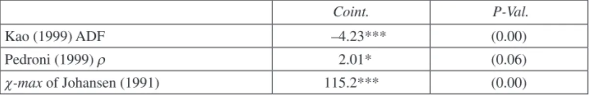
(13) Within and Between Panel Cointegration in the German Regional Output-Trade-FDI Nexus. 103. single-equation and system tests, with the most prominent operationalizations in time-series analysis being the Engle-Granger (1987) and Johansen (1991) VECM approaches, respectively. For this analysis, we apply the Kao (1999) and Pedroni (1999) panel ρ tests as residual based approaches in the spirit of the Engle-Granger and additionally a Fisher (1932) type test, where the latter combines the probability values for single cross-section estimates of the Johansen (1991) system approach 5. If we get evidence for a stable cointegration relationship among the variables, we are then able to move on and specify different regression models which are capable of estimating non-stationary panel data models including information in levels and first differences. Since we have rather limited time-series observations, this makes it hard to estimate individual models for each German region. A natural starting point would thus be to pool the time-series and cross-section data for purposes of estimation. However, this is only feasible if the data is actually «poolable» (see, e.g., Baltagi, 2008). Among the common estimation alternatives in this setting with small N and increasing T are the pooled mean group (PMG) and the dynamic fixed effects (DFE) model. While the PMG estimator allows for cross-section specific heterogeneity in the coefficients of the short run parameters of the model (see Pesaran et al., 1999), the DFE model assumes homogeneity of short and long-run parameters in the estimation approach. Given a consistent benchmark (such as the standard mean group estimator, see Pesaran & Smith, 1995), we are also able to test for the appropriateness of the pooling approach by means of standard Hausman (1978) tests. Table 3 first presents the results of the cointegration tests among output, trade and FDI, Table 4 then gives a detailed overview of the regression output for the PMG and DFE estimator using the sample period 1976 to 2005. Table 3.. Panel cointegration tests for regional output, trade and FDI in the aspatial model. Kao (1999) ADF Pedroni (1999) ρ. χ-max of Johansen (1991). Coint.. P-Val.. –4.23***. (0.00). 2.01*. (0.06). 115.2***. (0.00). Note: ***, **, * denote significance at the 1, 5 and 10% level. H0 for panel cointegration tests is the no-cointegration case. For the Johansen maximum eigenvalue test MacKinnon-Haug-Michelis (1999) p-values are reported. The test is applied to the null hypothesis of rank (r ≤ 0) against the alternative of (r + 1).. 5 The Fisher-type test can be defined as –2 ∑Ni= 1 log(φi) → χ22N, where φi is the p-value from an individual Johansen cointegration test for cross-section i. Here, we apply the Fisher test to the maximum eigenvalue (χ-max) of the Johansen (1991) approach, which tests the null hypothesis of r cointegration relationships against the alternative of (r + 1) relationships. At this point we restrict the Johansen approach to test the null hypothesis of rank ≤ 0. If the null hypothesis is rejected, for the underlying single cointegration vector we then assume that it has the form of a stylized output equation driven by trade and FDI as, e.g., outlined for the case of the augmented export base model outlined above.. 07-TIMO.indd 103. 22/2/12 11:22:42.

(14) 104. Mitze, T.. Table 4. Aspatial model estimates for the growth-trade-FDI Nexus Dep. Var.: ∆ y exit imit fdi outit fdi init. uit-1. ∆ yit-1 ∆ exit ∆ imit ∆ fdi outit ∆ fdi init Hausman Test χ 2(4) p-value STMI residuals p-value p b-value. PMG Long run estimates 1.02*** (0.337) -0.42* (0.224) -0.21 (0.157) 0.16 (0.118) Short run estimates -0.06*** (0.009) 0.29*** (0.048) -0.08** (0.038) 0.10*** (0.016) 0.07*** (0.019) 0.06*** (0.012) 15.29*** (0.00) 5.96*** (0.00) (0.00). DFE 0.78*** (0.299) -0.47 (0.323) -0.15 (0.235) 0.16 (0.169) -0.05*** (0.014) 0.33*** (0.048) -0.01 (0.033) 0.07*** (0.022) 0.06*** (0.013) 0.06*** (0.013) 0.01 (0.00) 7.45*** (0.00) (0.00). Note: ***, **, * denote significance at the 1, 5 and 10% level. Standard errors in brackets. The Hausman test checks for the validity of the PMG and DFE specifications against the MG estimation results. STMI is the spatio-temporal extension of the Moran’s I statistic, which tests for H0 of spatial independence among observations. Since we are dealing with a small number of cross-sections, we use standard as well as bootstrapped p-values of the test. The latter are marked by a «b».. If we first look at the panel cointegration tests in Table 3, we see that the Kao (1999) and Fisher-type Johansen (1991) tests clearly rejects the null hypothesis of no cointegration for the five variables employed. However, the result of the Pedroni pa nel ρ test is less clear cut. Here, we only get empirical support for a stable cointegration relationship at the 10% significance level. Regarding the estimated coefficients, the results in Table 4 show that we find a positive long-run effect of export activity on growth, both for the PMG and the DFE models. This is consistent with the exportled growth theory of regional economics. However, for imports, we find a negative impact on GDP, which is, however, only statistically significant at the 10% level.. 07-TIMO.indd 104. 22/2/12 11:22:42.

(15) Within and Between Panel Cointegration in the German Regional Output-Trade-FDI Nexus. 105. The models do not find any long-run causation from FDI activity (both inward and outward) to GDP. Looking at the short-run coefficients, we see that the coefficient of the error correction term is statistically significant and of expected sign, although the speed of adjustment to the long-run equilibrium is rather slow (around 5-6% per year). Though we do not find a statistical long-run impact of import and FDI activity on economic growth, there is a multidimensional positive short-run correlation from import and both FDI variables to output growth. The sole exception is export flows, for which we do not find any short-run effect in the DFE model and a reversed coefficient sign in the PMG model. If we finally check for the statistical appropriateness of the respective estimators, we see from the results of the Hausman m-statistic that only for the DFE model we cannot reject the null hypothesis of consistency and efficiency of the DFE relative to the benchmark mean group (MG) estimator 6. On the contrary, the PMG is found to be inconsistent. Thus, we conclude that the DFE is the preferred (aspatial) model specification in the context of the German growth-trade-FDI nexus. So far we did not account for the spatial dimension of the data. As Beenstock & Felsenstein (2010) point out, this may lead to a severe bias of the estimation results both in terms of the cointegration space of the variables as well as incomplete handling of spatial dependence in the model. To check for the appropriateness of our aspatial cointegration relationship from Table 4, we calculate a spatio-temporal extension to the Moran’s I statistic (thereafter labeled STMI) for the estimated models’ residuals, which has recently been proposed by Lopez et al. (2011). Since we are dealing with a small number of cross-sections, we compute both asymptotic as well as bootstrapped test statistics to get an indication of the degree of misspecification in the model. Lin et al. (2009) have shown that bootstrap based Moran’s I values are an effective alternative to the asymptotic test in small-sample settings. Details about the computation of the STMI and bootstrapped inference are given in the Appendix. As the results show, the STMI strongly rejects the null hypothesis of spatial independence among the observed regions for both the asymptotic as well bootstrapped-based test statistic using a distance matrix based on common borders among German states. In sum, these results may be seen as a first strong indication that the absence of explicit spatial terms in the regression may induce the problem of spurious regression. 5.2. Global Cointegration and SpECM. We now move on to an explicit account of the spatial dimension both in the long- and short-run specification of the model. First, we estimate the long-run equation for the relationship of GDP, trade, and FDI. The results for the augmented panel 6 We do not report regression results of the MG estimator here. They can be obtained from the author upon request. The MG estimator assumes individual regression coefficients in the short- and long-run and simply averages the coefficients over the individuals. Pesaran & Smith (1995) have shown that this results in a consistent benchmark estimator.. 07-TIMO.indd 105. 22/2/12 11:22:42.

(16) 106. Mitze, T.. cointegration tests and different estimation strategies are shown in Table 5 and Table 6, respectively. We start from a simple fixed effects specification. However, due to the inclusion of spatial lags, OLS estimation may lead to inconsistent estimates of the regression parameters (see, e.g., Fischer et al., 2009). Since eq.(2) takes the form of a general spatial Durbin model, it may be appropriately estimated by maximum likelihood (ML), which has recently been proposed for panel data settings in Beer & Riedl (2009). The estimator of Beer & Riedl (2009) makes use of a fixed-effects (generalized Helmert) transformation proposed by Lee & Yu (2010) and maximizes the log-likelihood function with imposed functional form for the individual variances to keep the number of parameters to be estimated small (for details, see Beer & Riedl, 2009). The authors show by means of a Monte Carlo simulation experiment that the SDM-ML estimator has satisfactory small-sample properties. Besides the SDM-ML model, which includes spatial lags of the endogenous and exogenous variables, we also estimate a spatial Durbin error model (SDEM), which includes spatial lags of the exogenous variables and a spatially lagged error term as well as estimate the SDM by GMM. Table 5. Panel cointegration tests for regional output, trade and FDI in spatially augmented model Kao (1999) ADF Pedroni (1999) ρ. χ-max of Johansen (1991). Coint.. P-Val.. –3.70***. (0.00). 2.74***. (0.00). 741.0***. (0.00). Note: ***, **, * denote significance at the 1, 5 and 10% level. H0 for panel cointegration tests is the no-cointegration case. For the Johansen maximum eigenvalue test MacKinnon-Haug-Michelis (1999) p-values are reported. The test is applied to the null hypothesis of rank (r ≤ 0) against the alternative of (r + 1).. Again, we first look at the obtained test results from the panel cointegration tests including spatial lags of the exogenous variables. The results in Table 5 give strong empirical evidence that the variables cointegrated. Compared to the aspatial specification the result of the Pedroni (1999) test is improved (statistically significant at the 1% level), indicating that the inclusion of spatial lags of exogenous variables is necessary to ensure a stable cointegration relationship for a regional economic model as already pointed out by Felsenstein & Beenstock (2010). Regarding the estimated coefficients, again we observe a positive effect from exports on GPD in the spatially augmented long-run relationship. The estimated elasti city is somewhat smaller compared to the aspatial estimators from above. Next to the direct export effect for the DFE, we also observe an indirect effect from the spatial lag of the export variable (ex*). That is, an increased export activity in neighboring regions also spills over and leads to an increased GDP level in the home region. The effect, however, becomes insignificant if we move from a simple FEM regression to a ML based estimator for the general spatial Durbin model (SDM) and spatial Durbin. 07-TIMO.indd 106. 22/2/12 11:22:42.

(17) Within and Between Panel Cointegration in the German Regional Output-Trade-FDI Nexus. 107. error model (SDEM) as well as the GMM approach in Table 6 7. All specifications show a significant direct effect of outward FDI on regional output. The latter can be associated with the FDI-led growth hypothesis. Additionally, the SDM-ML model also finds a significant positive coefficient for interregional spillovers from outward FDI stocks on the output level. The direct impact of import flows turns out to be insignificant. However, we get a significant negative coefficient for the indirect spillover effect (both for the FEM and SDM-ML), indicating that higher importing activity in neighboring regions are correlated with GDP levels in the own region. For inward FDI, we hardly find any direct or indirect spatial effect on GDP. While the partial derivatives of direct and indirect effects for each exogenous variable can be immediately assessed for the FEM and SDEM-ML results in TaTable 6. Dep. Var.: y. Spatially augmented long-run estimates of GDP, trade and FDI Spatial FEM 0.27***. exit. (0.098) 0.08. imit. (0.086) fdi outit. 0.28*** (0.040). fdi init. 0.04 (0.037). ex. * it. im*it. SDM-ML 0.49*** (0.089) –0.03 (0.106) 0.28*** (0.057) –0.01 (0.049). SDEM-ML 0.41***. SDM-GMM 0.55**. (0.076). (0.232). 0.06. 0.40. (0.072). (0.247). 0.19*** (0.029) 0.06** (0.028). 0.36** (0.158) –0.41 (0.258). 0.19*. 0.07. 0.05. (0.101). (0.049). (0.078). (0.320). –0.20**. –0.10**. 0.03. 0.33. (0.103). (0.042). (0.082). 0.04 (0.049). (0.032). (0.036). (0.084). fdi in*it. –0.01. –0.05*. –0.02. –0.01. (0.048). (0.029). (0.034). (0.147). y. error. * it. 0.04. (0.285). fdi out*it. * it. 0.18***. –0.02. –0.04. –0.23***. –0.06. (0.021). (0.582) 0.19*** (0.012). Note: ***, **, * denote significance at the 1, 5 and 10% level. Standard errors in brackets. The SDM-GMM uses up to two lags for the exogenous variables and their spatial lags, as well as the twice lagged value of the spatial lag of the endogenous variable.. We specify the GMM approach in extension to the ML estimators, since the model may be a good candidate for estimation of the time and spatial dynamic processes in the second step short-run specification. 7. 07-TIMO.indd 107. 22/2/12 11:22:43.

(18) 108. Mitze, T.. ble 6 8, LeSage & Pace (2009) have recently shown that for model specifications including a spatial lag of the endogenous variable, impact interpretation is more complex. Table 7 therefore additionally computes summary measures for the SDMML based on a decomposition of the average total effect from an observation into the direct and indirect effect. The table shows that there is a significant total effect of export flows on the regional GDP level, which can be almost entirely attributed to its direct effect. Imports and inward FDI are not found to have either a significant direct or indirect effect, while for the case of outward FDI, we find both a positive direct as well as indirect effect. The latter results contrast findings from the SDEMML, indicating a significant effect running from inward FDI to growth. As LeSage & Pace (2009) point out, we cannot directly judge about the validity of one of the two models, since the SDEM does not nest the SDM and vice versa. However, one potential disadvantage of the SDEM compared to the SDM is that it could result in severe underestimation of higher-order (global) indirect impacts (see LeSage & Pace, 2009, for details). We may thus argue that SDM-ML is the most reliable specification for the long-run estimation of the output-Trade-FDI system. Table 7.. Direct, indirect and total effect of variables in SDM-ML direct. indirect. exit. 0.52***. –0.07. imit. 0.03. –0.14. fdi outit. 0.21***. fdi init. 0.03. 0.17*** –0.08. total 0.46*** –0.11 0.37*** –0.05. Note: ***, **, * denote significance at the 1, 5 and 10%-level using simulated parameters as described in LeSage & Pace (2009).. We then move on and use the obtained long-run cointegration relationship in a SpECM framework for regional GDP growth. The estimation results of the SpECM are shown in Table 8. For estimation of the SpECM, we apply the standard DFE model, the SDM-ML from Beer & Riedl (2009), as well as the spatial dynamic GMM specification. The latter estimator explicitly accounts for the endogeneity of the time lag of the dependent variable by valid instrumental variables. Although the time dimension of our data is reasonably long, the bias of the fixed effects estimator may still be in order.9 The spatial dynamic GMM estimator using an augmented instrument set in addition to the aspatial version proposed by Arellano & Bond (1991) as well as Blundell & Bond (1998) has recently performed well in Monte Carlo simulations (see Kukenova & Monteiro, 2009) as well as in empirical applications (e.g., Bouayad-Agha & Vedrine, 2010). Valid moment conditions for instrumenting the spatial lag of the endogenous variable besides the time lag are given in the Ap8 This also holds for the SDM-GMM since the spatial lag coefficient of the dependent variable is insignificant. 9 Using Monte Carlo simulations, Judson & Owen (1999), for instance, report a bias of about 20% of the true parameter value for the FEM, even when the time dimension is T = 30.. 07-TIMO.indd 108. 22/2/12 11:22:43.

(19) Within and Between Panel Cointegration in the German Regional Output-Trade-FDI Nexus. Table 8.. Spatially augmented short-run estimates of GDP, trade and FDI}. Dep. Var.: ∆ y uit-1. DFE –0.16*** (0.025). u*it-1. 0.14*** (0.025). ∆ yit-1. 0.49*** (0.040). ∆ exit ∆ imit. ∆ im*it ∆ fdi out*it ∆ fdi in*it. –0.21***. (0.033). (0.034). –0.01 (0.012) 0.36*** (0.099). 0.20*** (0.036) 0.47*** (0.049). 0.06. 0.03. (0.051). (0.044). 0.10*** 0.09*** 0.06*** (0.012). ∆ ex*it. SDM-GMM. 0.04. (0.016). ∆ fdi init. SDM-ML –0.05*. (0.032) (0.024). ∆ fdi outit. 109. 0.06 (0.047) 0.07*** (0.025) 0.06*** (0.020). 0.14*** (0.011) 0.08*** (0.019) 0.06*** (0.011). 0.05**. 0.01. 0.02*. (0.021). (0.026). (0.010). –0.04*. –0.01. –0.04**. (0.019). (0.183). 0.01. 0.02. (0.009). (0.014). 0.01 (0.011). ∆ y*it. 0.06*** (0.011) 0.22***. (0.013) –0.02 (0.018) 0.01 (0.010) 0.11**. (0.036). (0.044). STMI residuals. –2.85***. –1.08. –1.41. p-value. (0.00). (0.14). (0.08). p b-value. (0.00). (0.84). (0.12). Note: ***, **, * denote significance at the 1, 5 and 10% level. Standard errors in brackets. SMTI is the spatio-temporal extension of the Moran’s I statistic, which tests for Ho of spatial independence among observations. Since we are dealing with a small number of cross-sections, we use standard as well as bootstrapped p-values of the tests. The latter are marked by a «b».. pendix. The inclusion of time and spatial lags in the SpECM results in a «time-spacesimultaneous» specification (see, e.g., Anselin et al., 2007). With respect to the included variables, all model specifications report qualitatively similar results. For the standard EC-term we get a highly significant regression parameter in the DFE- and GMM-based specification, which is of expected sign. Besides the results from the panel cointegration tests from Table 6, this is a further. 07-TIMO.indd 109. 22/2/12 11:22:43.

(20) 110. Mitze, T.. indication that GDP and the variables for internationalization activity co-move over time in a long-run cointegration relationship, where short-term deviations balance out in the long-run. For the size of the EC-term, the spatial dynamic GMM model comes closest to values typically found in the empirical literature, with about onefifth of short-run deviations being corrected after one year (see, e.g., Ekanayake et al., 2003). Also, the coefficient for the spatialized EC-term (u*) is significantly different from zero in the DFE and GMM specification. Looking at the short-run correlation between growth, trade, and FDI in Table 8, we see that both direct and indirect (spatial) forces are present. As for the direct effects, the results do not differ substantially from the aspatial SpECM specification in Table 4. We do not find any significant short-run effect from export activity on growth. However, all other variables are positively correlated with the latter. Looking more carefully at the spatial transformations of these variables, we see that a higher export activity has a positive spillover effect on the output growth of neighboring regions while imports have a negative indirect effect (in line with the long-run findings). We also check for the significance of spatial lags in the endogenous variable and the error term. Here we find that there are indeed spatial spillovers from an increased growth performance in neighboring regions, a result which mirrors related findings for German regional growth analysis (see, e.g., Niebuhr, 2000, as well as Eckey et al., 2007). This result is also supported by the significant and positive coefficient for the spatial lag of the error correction variable (u*). We do not find any sign for significant spatial autocorrelation left in the residuals of the SDM-ML and SDMGMM using the (bootstrapped) STMI test.. 6.. Conclusion. The aim of this paper was to analyze the role of within and between panel cointegration for the German regional output-trade-FDI nexus. While investigating the comovements among non-stationary variables is by now a common standard in panel time-series analysis, less attention has been paid to the importance of spatial lags in the long-run formulation of a regression model. Applying the novel concept of global cointegration, as recently proposed by Beenstock & Felsenstein (2010), enables us to estimate spatially-augmented error correction models (SpECM) for West German data between 1976 and 2005. Our results show that both direct as well as indirect spatial linkages among the variables matter when tracking their long-run co-movement. First, the regression results for the long-run equation give empirical support for a direct cointegration relationship among economic output and internationalization activity. In particular, export flows show a significant and positive long-run impact on GPD, supporting the export-led growth hypothesis from regional and international economics. Moreover, we also get evidence that outward FDI drives output in the long-run. Second, besides these direct effects, the latter variable is also found to exhibit significant positive spatial spillovers. In general, augmenting the model by spatial lags of the trade and FDI variables significantly increases the model perfor. 07-TIMO.indd 110. 22/2/12 11:22:43.

(21) Within and Between Panel Cointegration in the German Regional Output-Trade-FDI Nexus. 111. mance both regarding the applied panel cointegration tests as well as tests for spatial dependence in the regression residuals. Our results can thus be interpreted in similar veins as Beenstock & Felsenstein (2010), who find that the inclusion of spatial lags of exogenous variables may have important implications for the stability of a cointegration relationship among variables for a regional economic system. As empirical identification strategy in the spatially augmented model we employ both ML- as well as GMM-based estimators. Regarding the short-run determinants of economic growth, for most variables in the specified spatial error correction model (SpECM) we observe positive direct effects. Regarding the spatial lags, we find that a rise in the export flows in neighboring regions significantly increases the region’s own growth rate, while imports show negative feedback effects. Finally, we also find positive growth relationship among German regions if we augment the model by the spatial lag of the endogenous variables. This result mirrors earlier evidence for Germany, reporting positive spatial autocorrelation in regional growth rates. Our specified SpECM (both using ML as well as GMM with appropriate instruments for the time and spatial lag of the endo genous variable) passes residual based spatial dependence tests. For the latter, we use a spatio-temporal extension of the Moran’s I statistic, for which we calculate both asymptotic as well as bootstrapped standard errors.. References Anselin, L.; Le Gallo, J., and Jayet, H. (2007): «Spatial Panel Econometrics», in: Matyas, L.; Sevestre, P. (eds.): The Econometrics of Panel Data, Fundamentals and Recent Developments in Theory and Practice, 3.th ed., Dordrecht. Arellano, M., and Bond, S. (1991): «Some tests of specification for panel data: Monte Carlo evidence and an application to employment equations», Review of Economic Studies, vol. 58, pp. 277-297. Baldwin, R.; Martin, P., and Ottaviano, G. (1998): «Global income divergence, trade and industrialization: The geography of growth take-offs», NBER Paper, n.º 6458. Baltagi, B. (2008): Econometric Analysis of Panel Data, 4.th ed., Wiley. Baltagi, B.; Bresson, G., and Pirotte, A. (2007): «Panel unit root tests and spatial dependence», Journal of Applied Econometrics, vol. 22 (2), pp. 339-360. Baltagi, B.; Egger, P., and Pfaffermayr, P. (2007): «Estimating Models of Complex FDI: Are There Third-Country Effects?», Journal of Econometrics, vol. 140 (1), pp. 260-281. Barro, R., and Sala-i-Martin, X. (2004): Economic growth, 2.nd. ed., Cambridge. Beenstock M., and Felsenstein D. (2010): «Spatial Error Correction and Cointegration in Non Stationary Panel Data: Regional House Prices in Israel», Journal of Geographical Systems, vol. 12, n.º 2, pp. 189-206. Beer, C., and Riedl, A. (2009): «Modeling Spatial Externalities: A Panel Data Approach», Paper presented at the III, World Congress of the Spatial Econometrics Association, Barcelona. Blomstroem, M.; Globerman, S., and Kokko, A. (2000): «The Determinants of Host Country Spillovers from Foreign Direct Investment», CEPR Papers, n.º 2350. Blundell, R., and Bond, S. (1998): «Initial conditions and moment restrictions in dynamic panel data models», Journal of Econometrics, vol. 87, pp. 115-143.. 07-TIMO.indd 111. 22/2/12 11:22:43.

(22) 112. Mitze, T.. Bouayad-Agha, S., and Vedrine, L. (2010): «Estimation Strategies for a Spatial Dynamic Panel using GMM. A New Approach to the Convergence Issue of European Regions», Spatial Economic Analysis, vol. 5, n.º 2, pp. 205-227. Bowsher, C. (2002): «On Testing Overidentifying Restrictions in Dynamic Panel Data Models», Economics Letters, vol. 77 (2), pp. 211-220. Destatis (2009): «Außenhandel nach Bundesländern», various issues, German Statistical Office, Wiesbaden. Deutsche Bundesbank (2009): «Deutsche Direktinvestitionen im Ausland und ausländische Direktinvestitionen in Deutschland nach Bundesländern», Statistical Publication 10, Bestandserhebungen über Direktinvestitionen S130, various issues, Frankfurt. Dritsaki, M.; Dritsaki, C., and Adamopoulus (2004): «A Causal Relationship between Trade, Foreign Direct Investment and Economic Growth for Greece», American Journal of Applied Science, vol. 1 (3), pp. 230-235. Eckey, H. F.; Kosfeld, R., and Tuerck, M. (2007): «Regionale Entwicklung mit und ohne räumliche Spillover-Effekte», Jahrbuch für Regionalwissenschaften/Review of Regional Science, vol. 27, n.º 1, S. 23-42. Edwards, S. (1998): «Openness, productivity and growth: What do we really know?», Economic Journal, vol. 108 (2), pp. 383-398. Ekanayake, E.; Vogel, R., and Veeramacheneni, B. (2003): «Openness and economic growth: Empirical evidence on the relationship Between output, inward FDI, and trade», Journal of Business Strategies, vol. 20, n.º 1, pp. 59-72. Elhorst, J. P. (2010): «Applied Spatial Econometrics: Raising the Bar», Spatial Economic Analysis, vol. 5, n.º 1, pp. 5-28. Engle, R., and Granger, C. (1987): «Cointegration and Error Correction: Representation, Estimation and Testing», Econometrica, vol. 55, pp. 251-276. Everaert, G., and Pozzi, L. (2007): «Bootstrap-based bias correction for dynamic panels», Journal of Economic Dynamics & Control, vol. 31, pp. 1160-1184. Fisher, R. A. (1932): Statistical Methods for Research Workers, Edinburgh. Feenstra, R. (1990): «Trade and uneven growth», NBER Working Paper, n.º 3276. Fingleton, B. (1999): «Spurious Spatial Regression: Some Monte Carlo Results with Spatial Unit Roots and Spatial Cointegration», Journal of Regional Science, vol. 39, pp. 1-19. Fischer. M.; Bartkowska, M.; Riedl, A.; Sardadvar, S., and Kunnert, A. (2009): «The impact of human capital on regional labor productivity in Europe», Letters in Spatial and Resource Sciences, vol. 2 (2), pp. 97-108. Hamilton, J. D. (1994): Time Series Analysis, Princeton. Hansen, H., and Rand, J. (2006): «On the Causal Links between FDI and Growth in Develo ping Countries», World Economy, vol. 29 (1), pp. 21-41. Hausman, J. (1978): «Specification Tests in Econometrics», Econometrica, vol. 46, pp. 12511271. Hirschman, A. (1958): The strategy of economic development, New Haven. Im, K.; Pesaran, M., and Shin, Y. (2003): «Testing for unit roots in heterogeneous panels», Journal of Econometrics, vol. 115, pp. 53-74. Johansen, S. (1991): «Estimation and hypothesis testing of cointegration vectors in gaussian vector autoregressive models», Econometrica, vol. 59 (6), pp. 1551-1580. Judson, R., and Owen, A. (1999): «Estimating dynamic panel data models: a guide for ma croeconomists», Economics Letters, vol. 65, pp. 9-15. Kao, C. (1999): «Spurious Regression and Residual-Based Tests for Cointegration in Panel Data», Journal of Econometrics, vol. 90, pp. 1-44 Kelejian, H., and Prucha, I. (2001): «On the asymptotic distribution of the Moran I test statistic with applications», Journal of Econometrics, vol. 104, pp. 219-257.. 07-TIMO.indd 112. 22/2/12 11:22:43.

(23) Within and Between Panel Cointegration in the German Regional Output-Trade-FDI Nexus. 113. Kukenova, M., and Monteiro, J. A. (2009): «Spatial Dynamic Panel Model and System GMM: A Monte Carlo Investigation», MPRA Paper, n.º 11569. Lee, L., and Yu, J. (2010): «Estimation of spatial autoregressive panel data models with fixed effects», Journal of Econometrics, vol. 154 (2), pp. 165-185. LeSage, J., and Pace, K. (2009): Introduction to Spatial Econometrics, London. Lin, K.; Long, Z., and Ou, B. (2009): «Properties of Bootstrap Moran’s I for Diagnostic Tes ting a Spatial Autoregressive Linear Regression Model», Paper presented at the 3.th World Congress of the Spatial Econometrics Association, Barcelona. — (2010): «The Size and Power of Bootstrap Tests for Spatial Dependence in a Linear Regression Model», Computational Economics, forthcoming. Lopez, F.; Matilla-Garcia, M.; Mur, J., and Ruiz, M. (2011): «Four tests of independence in spatio temporal data», Papers in Regional Science, vol. 90 (3), pp. 663-685. MacKinnon, J.; Haug, A., and Michelis, L. (1999): «Numerical Distribution Functions of Likelihood Ratio Tests for Cointegration», in: Journal of Applied Econometrics, vol. 14, n,º 5, pp. 563-577. MacKinnon, J. (2002): «Bootstrap inference in econometrics», Canadian Journal of Econo mics, vol. 35, n.º 4, pp. 616-645. Makki, S., and Somwaru, A. (2004): «Impact of Foreign Direct Investment and Trade on Economic Growth: Evidence from Developing Countries», American Journal of Agricultural Economics, vol. 86 (3), pp. 793-801. Martin, P., and Ottaviano, G. (1996): «Growth and Agglomeration», CEPR Discussion Paper, n.º 1529. Mitze, T. (2012): «Empirical Modelling in Regional Science: Towards a Global Time-SpaceStructural Analysis», Lecture Notes in Economics and Mathematical Systems, vol. 657, Berlin et al.: Springer. Niebuhr, K. (2000): «Räumliche Wachstumszusammenhänge. Empirische Befunde für Deutschland», HWWA Discussion Paper, n.º 84. OECD (2002): «Foreign direct investment for development: Maximizing benefits, minimizing costs», Paris. Ozturk, I. (2007): Foreign Direct Investment - Growth Nexus: A Review of the Recent Literature, International Journal of Applied Econometrics and Quantitative Studies, vol. 4-2, pp. 79-98. Ozyurt, S. (2008): «Regional Assessment of Openness and Productivity Spillovers in China from 1979 to 2006: A Space-Time Model», Working Papers, n.º 08-15, LAMETA, University of Montpellier. Pedroni, P. (1999): «Critical Values for Cointegration Tests in Heterogeneous Panels with Multiple Regressors», Oxford Bulletin of Economics and Statistics, vol. 61, pp. 653-670. Pesaran, M. H. (2007): «A simple panel unit root test in the presence of cross-section depen dence», Journal of Applied Econometrics, vol. 22 (2), pp. 265-312. Pesaran, M. H., and Smith, R. (1995): «Estimating long-run relationships from dynamic heterogeneous panels», Journal of Econometrics, vol. 68, pp. 79-113. Pesaran, M. H.; Shin, Y., and Smith, R. (1999): «Pooled Mean Group Estimation of Dyna mic Heterogeneous Panels», in: Journal of the American Statistical Association, vol. 94, pp. 621-634. Rivera-Batiz, L., and Xie, D. (1993): «Integration among unequals», Regional Science and Urban Economics, vol. 23, pp. 337-354. Roodman, D. (2009): «How to Do xtabond2: An introduction to difference and system GMM in Stata», Stata Journal, vol. 9 (1), pp. 86-136. Romer, P., and Rivera-Batiz, L. (1991): «Economic Integration and endogenous growth», Quarterly Journal of Economics, vol. 106, pp. 531-555. Statistisches Bundesamt (1970): «Eisenbahnverkehr», Fachserie H, Reihe 4. Tondl, G. (2001): Convergence after divergence?, Berlin et al.. 07-TIMO.indd 113. 22/2/12 11:22:43.

(24) 114. Mitze, T.. VGRdL (2009): «Volkswirtschaftliche Gesamtrechnungen der Bundesländer» (Regional Accounts for German States), available at https://vgrdl.de. Wang, C.; Liu, S., and Wei, Y. (2004): «Impact of Openness on Growth in Different Country Groups», World Economy, vol. 27 (4), pp. 567-585. Wagner, M., and Hlouskova, J. (2009): «The Performance of Panel Cointegration Methods: Results from a Large Scale Simulation Study», Econometric Reviews, vol. 29 (2), pp. 182223. Won, Y., and Hsiao, F. (2008): «Panel Causality Analysis on FDI - Exports - Economic Growth Nexus in First and Second Generation ANIEs», The Journal of the Korean Economy, vol. 9, n.º 2, pp. 237-267.. Appendix A.1. Bootstrapping the Spatio-Temporal Extension of Moran’s I. Recently, different attempts have been made to improve statistical inference based on the Moran’s I statistic to detect spatial dependence in the data. First, Lin et al. (2009 & 2010) have shown that the power of Moran’s I statistic can be enhanced in small sample settings if bootstrapped test statistics are calculated instead of their asymptotic counterparts. Second, Lopez et al. (2011) have extended Moran’s I to the case of spatio-temporal data. The authors label the extended version as the «STMI test». In the following, we will combine both proposals for the application in spatial panel data settings with a small number of cross-sections. We thus first sketch the STMI test and then build a «wild» bootstrap version of the test in the spirit of Lin et al. (2009). The STMI test proposed by Lopez et al. (2011) is a straightforward extension of the cross-section test. In the latter setting, Moran’s I can be defined as I=. N S. ∑. r ≠s. ( yr − y ) wrs ( ys − y ). ∑. R. (y − y) r =1 r. (6). where y– is the sample mean for a variable y, wrs is the (r,s) element of a spatial weighting matrix W, N is the total number of cross-sections and S is a measure of overall connectivity for the geographical system. The null hypothesis of Moran’s I is the absence of correlation between the spatial series yr with r = 1, …, N and its spatial lag ∑ Ns= 1 wrs ys. Building upon I and a measure for its standard deviation, Moran’s I statistic is shown to be asymptotically normal with (see Lopez et al. (2011) as well as Kelejian & Prucha, 2001, for details) I ∼ N (0,1). Var ( I ). 07-TIMO.indd 114. (7). 22/2/12 11:22:43.

(25) Within and Between Panel Cointegration in the German Regional Output-Trade-FDI Nexus. 115. As Lopez et al. (2011) point out, it is not strictly necessary to restrict the application of Moran’s I to just one time period. Starting from a model with T consecutive cross-sections with N observations in each of them, stacked in an (NT x 1) vector, the authors show that the spatio-temporal version of Moran’s I can be computed as * NT ∑ ( t ,s )≠( r ,k )( yts − y ) w( t −1) T + s ,( r −1) T + k ( yrk − y ) , STMI = S ∑ ts( yts − y )2. (8). where yts is a spatio-temporal process with t ∈ Z and s ∈ S, where Z and S are sets of time and spatial coordinates with cardinality |Z|=T and |S| = R, respectively. Each element w* is taken from the following weighting matrix:. * WNT. WN   IN  0 =    0   0. 0 WN IN  0 0. 0 0 WN  0 0. … 0 … 0 … 0   … WN … IN.         WN  0 0 0  0. (9). where the cross-section based spatial weighting matrix of order N x N appears along the main diagonal and the diagonal below the main diagonal contains the temporal weighting matrix IN. The latter is defined as the identity matrix of order N (for further details, see Lopez et al., 2011). In a Monte Carlo simulation, Lopez et al. (2011) show that the STMI test is robust to different types of distribution functions and has satisfactory finite sample properties. Building upon the findings in Lin et al. (2009), we additionally develop a «wild» bootstrap based test version for the STMI, which is implemented through the follo wing steps: ^. Step 1: Estimate the residuals ê it as ê it = y – V d for the spatial or aspatial esti^ mator with regressors V and coefficients d (either short- or long-run specification) in focus and obtain a value for the STMI. Save the obtained STMI. Step 2:. Re-scale and re-center the regression residuals e~it according to  eit eit = , (1 − hit )1/ 2. (10). where hit is the model’s projection matrix so that a division by (1 – hit)1/2 ensures that the transformed residuals have the same variance (for details, see MacKinnon, 2002).. 07-TIMO.indd 115. 22/2/12 11:22:44.

(26) 116. Mitze, T.. Step 3: Choose the number of bootstrap samples B and proceed as follows for any j sample with j = 1, …, B: Step 3.1: According to the wild bootstrap procedure, multiply e~it with v~it, where the latter is defined as a two-point distribution (the so-called Rademacher distribution) with  1 with probability 1/2 ν it =  obability 1/2 −1 with pro. (11). Step 3.2: For each of the i = 1, …, N cross-sections, draw randomly (with replacement) T observations with probability 1/T from e~it × v~it to obtain e~*it. Step 3.3:. Generate a bootstrap sample for variable y (and its spatial lag) as yit* = V *δˆ + eit*. (12). where V * = (Wy*it,y*it–1}, X) and, for a time-dynamic specification, initialization as y*i0 = yi0. Thus, for a regression equation with a lagged endogenous variable, we condition on the initial values of yi0, the exogenous variables X, and the spatial weighting matrix W 10. Step 3.4: Obtain the residuals from the regression including y* and V *, calculate the bootstrap based STMI*. The full set of resulting bootstrap test statistics are STMI*1, STMI*2, …, STMI*B. From the empirical distribution, we can then calculate p-values out of the nonparametric bootstrap exercise in order to perform hypothesis testing. There are various ways to do so. Lin et al. (2009), for instance, express equal-tail p-values for STMI* as 1 B  1 B P* ( STMI * ) = 2 min ∑C ( STMI *j ≤ STMI ), ∑C ( STMI *j > STMI ) , B j =1  B j =1 . (13). where C(.) denotes the indicator function, which is equal to 1 if its argument is true and zero otherwise. Then, given a nominal level of significance α, we compare P*(STMI*j) with α. Following Lin et al. (2009), one can reject the null hypothesis of no spatial dependence if P* (STMI*j) < α.. 10 See, e.g., Everaert & Pozzi (2007) for the treatment of initial values to bootstrap dynamic panel data processes. In the following, by default, we generate y* based on the long-run cointegration specification, where we do not face the problem of time dynamics in the bootstrapping exercise. However, we additionally need to account for the generated error term and its spatial lag as explanatory regressors in the short-run equation.. 07-TIMO.indd 116. 22/2/12 11:22:44.

(27) Within and Between Panel Cointegration in the German Regional Output-Trade-FDI Nexus. 117. A.2. Moment Conditions for the Spatial Dynamic GMM Model. The use of GMM-based inference in dynamic panel data models is a common practice in applied research. Most specifications rest on instruments sets as proposed by Blundell & Bond (1998). Their so-called system GMM (SYS-GMM) approach combines moment conditions for the joint estimation of a regression equation in first differences and levels. The latter part helps to increase the efficiency of the GMM methods compared to earlier specifications solely in first differences (e.g., Arellano & Bond, 1991). Subsequently, extensions of the SYS-GMM approach have been proposed, which make use of valid moment conditions for the instrumentation of the spatial lag coefficient of the endogenous variable (see, e.g., Kukenova & Monteiro, 2009, Bouayad-Agha & Vedrine, 2010). Kukenova & Monteiro (2009) have also shown, by means of Monte Carlo simulations, that the spatial dynamic SYS-GMM model exhibits satisfactory finite sample properties. For the purpose of this analysis, we focus on appropriate moment conditions for the time-space simultaneous model including a time and spatial lag of the endoge nous variable. Instruments can be built based on transformations of the endogenous variable as well as the set of exogenous regressors. Assuming strict exogeneity of current and lagged values for any exogenous variable xi,t, then the full set of potential moment conditions for the spatial lag of yi,t is given by First differenced equation:   E  ∑ wij × yi, t − s ∆ui, t  = 0 t = 3,...,T s = 2,...t − 1,  i≠ j . (14).   E  ∑ wij × xi, t + / − s ∆ui, t  = 0 t = 3,...,T ∀s.  i≠ j . (15). Level equation:   E  ∑ wij × ∆yi, t −1 ui, t  = 0 t = 3,...,T ,  i≠ j . (16).   E  ∑ wij × ∆xi, t ui, t  = 0 t = 2,...,T.  i≠ j . (17). One has to note that the consistency of the SYS-GMM estimator relies on the validity of these moment conditions. Moreover, in empirical application we have to. 07-TIMO.indd 117. 22/2/12 11:22:44.

(28) 118. Mitze, T.. carefully account for the «many» and/or «weak instrument» problem typically associated with GMM estimation, since the instrument count grows as the sample size T rises. We thus put special attention to this problem and use restriction rules specifying the maximum number of instruments employed as proposed by Bowsher (2002) and Roodman (2009).. 07-TIMO.indd 118. 22/2/12 11:22:44.

(29)