Detection of classifier inconsistencies in image steganalysis
9
0
0
Texto completo
(2) Detection of Classifier Inconsistencies in Image Steganalysis Daniel Lerch-Hostalot David Megías Internet Interdisciplinary Institute (IN3), Universitat Oberta de Catalunya (UOC), CYBERCAT-Center for Cybersecurity Research of Catalonia Castelldefels, Barcelona, Spain {dlerch,dmegias}@uoc.edu. ABSTRACT In this paper, a methodology to detect inconsistencies in classification-based image steganalysis is presented. The proposed approach uses two classifiers: the usual one, trained with a set formed by cover and stego images, and a second classifier trained with the set obtained after embedding additional random messages into the original training set. When the decisions of these two classifiers are not consistent, we know that the prediction is not reliable. The number of inconsistencies in the predictions of a testing set may indicate that the classifier is not performing correctly in the testing scenario. This occurs, for example, in case of cover source mismatch, or when we are trying to detect a steganographic method that the classifier is no capable of modelling accurately. We also show how the number of inconsistencies can be used to predict the reliability of the classifier (classification errors).. KEYWORDS Steganalysis, Cover Source Mismatch, Machine Learning. 1. INTRODUCTION. Steganography is a collection of techniques to embed secret data into apparently innocent objects. Nowadays, these objects are mainly digital media, and the most common carriers for steganography are digital images because of their widespread use. On the other hand, steganalysis refers to different techniques used to detect messages previously hidden using steganography. Most steganalytic methods in the state of the art use machine learning [3, 6, 7]. In machine learning-based steganalysis, firstly, a (training) set of known cover and stego images is used to train a classifier. Later on, this classifier is used to predict the images of a testing set as cover or stego. This approach works very well in laboratory conditions, that is, if the set of training images is similar to that of the testing images used by the steganographer to hide secret data. However, in the real world, the set of media used by the steganographer might be quite different from that used to train the classifier [12]. This occurs, for example, when the images in the testing set are not well represented in the training set. Some examples of this mismatch occur if the testing images are taken using a different camera or resolution; if they are compressed, zoomed or improved through filters; or if they were taken in very different conditions. In steganalysis, this problem is known as cover source mismatch (CSM) and was initially reported in [4]. There are other situations that lead to inaccurate predictions. For example, stego source mismatch (SSM) occurs when some embedding parameter, such as the exact payload [20], differ between the training and the testing datasets.. Different approaches to the CSM problem have been proposed. During the BOSS competition [1], some participants tried an approach called “training on a contaminated database”, which consists in denoising images from the testing set and including them in the training set [8]. A different approach is to make the training set as complete as possible. In [18], the authors trained a classifier with a huge variety of images. Due to the high time and memory requirements, this was carried out using on-line classifiers. In [14], three different strategies are presented: (1) training with a mixture of cover sources; (2) using different classifiers trained with different sources and testing with the closest source; and (3) taking the second approach but testing each image separately using the closest source. The islet approach [19], introduces a pre-processing step consisting in organizing the images in clusters and assigning a steganalyzer to each cluster. In [23], a scheme to efficiently construct a large and representative training set is proposed. Finally, in [16], an unsupervised steganalytic method was proposed that does not require a training set, bypassing the CSM problem. In supervised machine learning-based steganalysis, we need a database of images to construct the training set and a validation set to determine the classification accuracy results. The creation of this database is a fundamental part of the process. Usually, this is carried out by collecting pictures taken with different cameras and models, taken in different lighting conditions, compressed with different algorithms and compressing ratios, processed with different filters, modified by optical or digital zoom, etc. If we create a database with pictures taken by a team of people with their cameras and with a specific set of filters, zooms, compression algorithms and so on, this will be a biased procedure, and such a selection can never represent the entire population of possible images. Even if we decide to download random images from the Internet, the combination of cameras, models, filters, compression ratios, light conditions, and so on, is too large and it is almost impossible to obtain a representative enough dataset. The current approach to solve this problem consist in building a very large and heterogeneous dataset, as described in [5]. By taking such an approach, the steganalyst expects that the trained classifier (usually a convolutional neural network) will learn a collection of features that are universal to all images and, consequently, good enough to classify images taken under conditions different from those of the training set. Although this approach is often successful, we think that it is convenient to test other solutions to the problem. In this paper, we explore an alternative approach. The proposed approach is based on the ideas of [16], which are extended here to detect samples that lead to classification inconsistencies. Thus, the suggested method stems from obtaining.
(3) additional training and testing sets by sequential random data embedding. Those additional sets are used here to detect inconsistencies in the classification. We present a method in the context of batch steganography [11], that is, when we are analyzing a set of images from a suspicious source. The rest of this paper is organized as follows. Section 2 introduces some relevant concepts that are used in the proposed method. Section 3 presents the proposed method. Experimental results obtained with the proposed method for different image databases, embedding algorithms and steganalytic classifiers (including CSM cases) are presented in Section 4. Finally, Section 5 summarizes the conclusions and suggests some directions for further research.. 2. PRELIMINARIES. We consider a targeted scenario in which the embedding algorithm and the approximate embedding rate –but not the secret key– are assumed to be known (at least approximately) by the steganalyst. Using the same steganographic algorithm and embedding bit rate, new (random) data can be hidden into any image with a different (random) secret key. Given a set of cover images, they can be used to build a training database by embedding random data to obtain a training database consisting of a half of cover and a half of stego images. This set is called Atrain . If a feature extraction-based machine learning algorithm is applied (not all the machine learning algorithms need feature extraction [3]), we need to extract the features of the images. The usual methodology in machine learning-based steganalysis is to use the set Atrain to train a classifier. Then, this classifier can be used to classify a testing set Atest , that is, a set of images for which we do not have a priori information whether they are cover or stego. The proposed methodology uses an additional set, B train , defined as suggested in [16]. The set B train is the result of hiding random data into all the images of the set Atrain using the targeted embedding algorithm, the approximate embedding bit rate and random keys. As a result, we have a set Atrain , which contains cover and stego images, and a set B train , which contains stego and “double stego” images. Now, we introduce the following notation: let α i be a sample from the set Atrain and βi be the corresponding sample from the set B train , whereby βi = Embed(α i , Bitrate). “Embed” stands for embedding a random message, using a random key and the targeted steganographic algorithm, and “Bitrate” is the known (or approximated) embedding bit rate. Similarly, from the images in Atest , we build an additional set B test following the same procedure: ai and bi stand for samples of the training sets Atest and B test , respectively, with bi = Embed(ai , Bitrate). The only difference with respect to the training sets is that we do not know the classes (labels) of the images of the testing sets. In other words, we know that Atest possibly contains both cover and stego images, and that B test possibly contains stego and “double stego” images, but we do not know the class of each image. Finally, we assume that there is a classifier fˆA (and a feature extractor if needed) that can split images into cover (CA ) and stego (SA ) classes with an acceptable probability of error. Similarly, we. assume that we have another classifier fˆB that can split images into stego (SB ) and “double stego” (DB ) classes, Table 1: Number of pixels modified by ±1 and ±2 for 1,000 images after the first and the second embeddings. “ALGO”/“BR”: embedding algorithm and bit rate (bpp) 1 embedding. 2 embeddings. ALGO. BR. ±1. ±2. ±1. ±2. HILL HILL UNIWARD UNIWARD LSBM. 0.4 0.2 0.4 0.2 0.2. 22,582,706 9,897,485 19,509,940 8,523,446 27,528,954. 0 0 0 0 0. 33,993,485 16,112,459 32,748,639 15,139,023 49,277,814. 2,819,705 933,376 1,563,635 477,200 1,439,498. The assumption of the existence of fˆB that can split images into stego (SB ) and “double stego” (DB ) classes needs some discussion. After all, both SB and DB classes are formed by stego images with more or less information hidden into them. Usually, in the spatial domain, steganographic algorithms embed information by carrying out a ±1 operation in some specific pixels. In a second embedding, the steganographic algorithm may choose an already modified pixel to hide additional information. Thus, in addition to ±1 changes, there is some probability of a ±2 operation for a few pixels. In the particular case of adaptive embedding, a probability map indicates the areas that will be selected for hiding information. These probability maps are quite similar for the cover and stego versions of the same image. Therefore, the algorithm tends to hide information in the same pixels. This increases the differences between the features of stego and “double stego” images. These differences become more detectable with greater embedding ratios. One can conclude that the patterns of pixels (and its neighbours) generated after the second embedding will be different from those of a single embedding, and a good enough classifier can take advantage of those differences. In Table 1, the number of ±1 and ±2 variations after embedding messages with different algorithms and bit rates in 1,000 images randomly selected from the BOSS base are shown. We have included an experiment with LSB matching to show that even with non-adaptive steganography, the number of ±2 variations is not negligible. It can be observed that the number of ±2 variations is relatively large and and that the final number of ±1 changes is higher after the second embedding. These two factors help the classifier to split stego and “double stego” images. Even in the case of LSB matching, which does not use a probability map that forces the algorithm to hide data in the same positions, the number of ±2 variations is quite high. To analyze the relevance of ±2 changes for the classification, we trained a classifier fˆB using the BOSS database and the HILL embedding algorithm with a bit rate of 0.4 bits per pixel (bpp). We obtained a classification error of 0.2770. Next, we trained the classifier with the same images after replacing the ±2 changes by their respective ±1 values. In this case, we obtained an error of 0.3160, which is slightly worse. Therefore, it can be seen that, although the influence of ±2 changes in the classification is very significant, the increase in the number of ±1 changes is enough to split both classes..
(4) Atrain C. B train. Atrain. S αj. D. B train. C. S. ai. bi. αi. βi. αn. αl. αk. βk. βn βl. aj. αm. Testing cover sample Testing stego sample. (a) Atrain and B train sets. C. (b) Consistent predictions. B train. Atrain. S. D. ai. bi. C. Atrain D. ai. C. B train S. D. bi bj. bj. ai. bj. Testing cover sample Testing stego sample. (c) Undetectable inconsistencies. 3. B train S. aj aj. bj. βm. Training cover sample Training stego sample. Atrain. D. βj. Testing sample. (d) Some F 1 -detectable inconsistencies Fig. 1. Graphical representation of the proposed method. PROPOSED METHOD. This section outlines the method proposed to detect the number of inconsistencies occurred during classification. We also propose a mechanism to predict the error incurred by the classifier based on the number of such inconsistencies. Usually, in machine learning-based steganalysis, when we know the embedding algorithm and the approximate embedding rate, the testing set is expected to be classified with some (hopefully low) probability of error [7]. If this idea is extended to the sets introduced in the previous section, we have a tool that can be used to detect inconsistencies in classification. Since there is a bijection between the elements of Atest and B test , if an image is classified as cover using fˆA , the corresponding image in B test should be classified as stego (not “double stego”) using fˆB . Similarly, if an image in Atest is classified as stego using fˆA , we expect the same image in B test to be classified as “double stego” if we use fˆB . We call “inconsistency” to a classification result that does not meet these requirements. The classification constraints described above are used to define filters. The filter described in the previous paragraph is denoted as F 1 , and consists in classifying ai using fˆA and bi using fˆB to check. Testing sample. (e) F 2 -detectable inconsistencies. whether the two classification results are consistent:. F 1 (i) ≡. If fˆA (ai ) = SA , . If ( fˆB (bi ) , DB ) then output “inconsistency”,. Otherwise, . If ( fˆB (bi ) , SB ) then output “inconsistency”.. In Fig.1a, we can see a graphical representation of the classes. A consistent classification is represented in Fig.1b. In Fig.1d, we can see different inconsistencies that can be detected with the filter F 1 . Now, we can consider the case in which fˆA is used to classify ai ∈ Atest and the classification result is stego. If we classify ai ∈ Atest using fˆB , we expect that it is classified also as stego (not as “double stego”). If ai is classified as stego using fˆA and as “double stego” by fˆB , there is an inconsistency. In fact, if ai corresponds to a cover image, it would not be consistent that ai is classified by fˆB as “double stego” either. Hence, for any image ai in Atest , the output of fˆB taking ai as input must be always stego and never “double stego”. The same idea can be applied to inconsistencies for the set B test . If we use fˆA to classify any sample bi ∈ B test , we expect bi to be classified as stego (and never as cover). This kind of filter is.
(5) denoted as F 2 (represented in Fig.1e): F 2 (i) ≡. ˆ If f B (ai ) , SB , . then output “inconsistency”,. If fˆ (b ) , S , A i A . then output “inconsistency”.. Note that there is a case that cannot be detected with these filters: an image that is misclassified by all the classifiers. A graphical representation of this case is provided in Fig.1c.. 4. EXPERIMENTAL RESULTS. The experimental validation of the method has been performed with different datasets selecting images from the following databases: • The BOSS database is the set of images from the Break Our Steganographic System! competition [1]. This database is formed by 10,000 cover images taken with seven different cameras, with a size of 512×512 pixels. For JPEG experiments, we have compressed the images to qualities 75 and 95. In these cases, we refer to the datasets as BOSS-J75 and BOSSJ95, respectively. • The BOWS2 database is the set of images from the Break Our Watermarking System 2nd Ed. competition [2]. This database is formed by 10,000 cover images with a size of 512 × 512 pixels. For JPEG experiments, we have compressed the images to qualities 75 and 95. In these cases, we refer to the datasets as BOWS2-J75 and BOWS2-J95, respectively. • The ALASKA database is the set of images from the Alaska competition [5]. This database is formed by 50,000 cover images with different sizes. For our experiments, we have selected 10,000 images randomly and we have cropped the center with a size of 512 × 512 pixels, and then converted them to gray scale. For JPEG experiments, we compressed the cropped images to qualities 75 and 95. In these cases, we refer to the datasets as ALASKA-J75 and ALASKA-J95, respectively. For the experiments with SRNet [3], all these datasets have been resized to 256 × 256 pixels. All the databases were randomly separated into two sets: a set for training and a set for testing. All the experiments, but Experiment 2 in Table 2, use 9,500 images for training. Experiment 2 uses 5,000 images for training. The number of images used for testing varies among different experiments and it is provided in the different tables. These sets have been formed by the original cover images and the same images with an embedded message, using a random key. In this way, we have tested the CSM problem by using a training set from a database and a testing set from another one. The experiments detailed below have been carried out for three different spatial domain steganographic algorithms: UNIversal WAvelet Relative Distortion (UNIWARD) [10], HIgh-pass, Lowpass, and Low-pass (HILL) [17] and LSB matching (LSBM) [21]; and for two different transformed domain steganographic algorithms: UED [9] and J-UNIWARD [10]. We were mainly interested in the results of the state-of-the-art algorithms, but we have also performed experiments using LSB matching to have a reference of a non-adaptive algorithm. For these experiments, we have used a different random key for each stego image. The experiments have been performed using. the same algorithm and embedding bit rate for the training and the testing sets unless explicitly noted otherwise. Thus, the proposed scenario is for a known algorithm and known embedding rate attack. To analyze the proposed approach, we have used the well known Rich Models (RM) framework [7] for the spatial domain and Gabor Filter Residuals (GFR) [22] for the transformed domain, with Ensemble Classifiers (EC) [13]. These classifiers meet the requirements introduced in Section 3, i.e., they make it possible to classify the sets Atest (as CA and SA ) and B test (as SB and DB ) for UNIWARD, HILL, LSBM, UED and similar algorithms. When using RM+EC, we do not expect the proposed approach to work with algorithms designed to overcome this framework, such as [15], because the proposed method depends on the underlying classifier. We have also performed some experiments using the state-ofthe-art convolutional neural network (CNN) described in [3].. 4.1. Classifier Inconsistencies. The results obtained detecting inconsistencies are presented in this section. In Tables 2-8, the results for different experiments are shown. The first column indicates the experiment number (used for references along the text). The first few columns show the algorithm and bit rate used for embedding, the databases used for training and for testing, the number of cover and stego images contained by the testing set, and the method used for classification. For example, the first row of the first experiment shows the results obtained using images from BOSS for training and images from the same database for testing (500 cover and 500 stego images), for HILL steganography with a 0.4 bpp embedding bit rate, using Rich Models with Ensemble Classifiers as the classification method. The results are computed first without applying any filter and next with the proposed filters. The column error (Err) is the result of the classification error using the reported method. This error is computed as: FP + FN Err = , FP + FN + TP + TN where TP are the true positives, TN the true negatives, FP the false positives and FN the false negatives. These values are also provided in Tables 2-8. When the filters are applied, we also show the number of inconsistencies (INC) obtained during the classification, and which of those correspond to images classified by fˆA as cover (INCC ) or as stego (INCS ). When there is no CSM (for example, in the first row of Experiment 1-A of Table 2) the number of inconsistencies is quite lower compared to the cases with CSM (e.g. the first rows of Experiments 1-B and 1-C of Table 2). It can also be observed that the number of inconsistencies increases with lower embedding bit rates (Experiment 5 of Table 4). This occurs because the proposed method does not only reveal if there is CSM, but whether the classifier is working well with the testing database or not. This information can be used to make a good prediction about he classification errors, as detailed belown.. 4.2. Prediction of the Classification Error. In this section, we show how to carry out a prediction of the classification error. For this purpose, we assume that the standard steganalyzer is classifying randomly the samples that are not well.
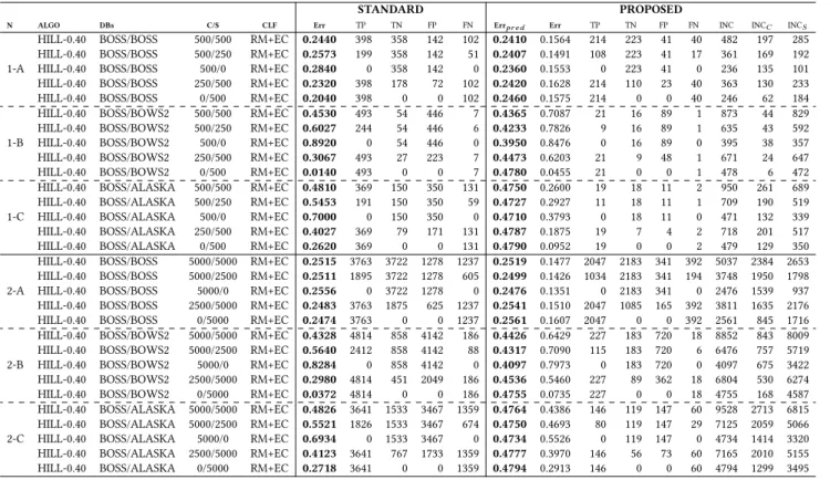
(6) Table 2: Classification results for standard RM+EC (without filters) and for the proposed method (with filters). “N”: number of experiment, “ALGO”: name of the embedding algorithm and embedding bit rate (bpp), “DBs”: training/testing databases, “C/S”: number of cover and stego images in the testing set , “CLF”: classification method used, “Err”: true classification error, {“TP”, “TN”, “FP”, “FN”}: true and false positives and negatives, “INC”: number of inconsistencies, “INCC ”: number of inconsistencies for images predicted as cover, and “INCS ”: number of inconsistencies for images predicted as stego STANDARD N. 1-A. 1-B. 1-C. 2-A. 2-B. 2-C. ALGO. DBs. HILL-0.40 HILL-0.40 HILL-0.40 HILL-0.40 HILL-0.40 HILL-0.40 HILL-0.40 HILL-0.40 HILL-0.40 HILL-0.40 HILL-0.40 HILL-0.40 HILL-0.40 HILL-0.40 HILL-0.40 HILL-0.40 HILL-0.40 HILL-0.40 HILL-0.40 HILL-0.40 HILL-0.40 HILL-0.40 HILL-0.40 HILL-0.40 HILL-0.40 HILL-0.40 HILL-0.40 HILL-0.40 HILL-0.40 HILL-0.40. BOSS/BOSS BOSS/BOSS BOSS/BOSS BOSS/BOSS BOSS/BOSS BOSS/BOWS2 BOSS/BOWS2 BOSS/BOWS2 BOSS/BOWS2 BOSS/BOWS2 BOSS/ALASKA BOSS/ALASKA BOSS/ALASKA BOSS/ALASKA BOSS/ALASKA BOSS/BOSS BOSS/BOSS BOSS/BOSS BOSS/BOSS BOSS/BOSS BOSS/BOWS2 BOSS/BOWS2 BOSS/BOWS2 BOSS/BOWS2 BOSS/BOWS2 BOSS/ALASKA BOSS/ALASKA BOSS/ALASKA BOSS/ALASKA BOSS/ALASKA. CLF. Err. TP. TN. FP. FN. Errpr ed. Err. TP. TN. FP. FN. INC. INCC. INCS. 500/500 500/250 500/0 250/500 0/500 500/500 500/250 500/0 250/500 0/500 500/500 500/250 500/0 250/500 0/500 5000/5000 5000/2500 5000/0 2500/5000 0/5000 5000/5000 5000/2500 5000/0 2500/5000 0/5000 5000/5000 5000/2500 5000/0 2500/5000 0/5000. RM+EC RM+EC RM+EC RM+EC RM+EC RM+EC RM+EC RM+EC RM+EC RM+EC RM+EC RM+EC RM+EC RM+EC RM+EC RM+EC RM+EC RM+EC RM+EC RM+EC RM+EC RM+EC RM+EC RM+EC RM+EC RM+EC RM+EC RM+EC RM+EC RM+EC. 0.2440 0.2573 0.2840 0.2320 0.2040 0.4530 0.6027 0.8920 0.3067 0.0140 0.4810 0.5453 0.7000 0.4027 0.2620 0.2515 0.2511 0.2556 0.2483 0.2474 0.4328 0.5640 0.8284 0.2980 0.0372 0.4826 0.5521 0.6934 0.4123 0.2718. 398 199 0 398 398 493 244 0 493 493 369 191 0 369 369 3763 1895 0 3763 3763 4814 2412 0 4814 4814 3641 1826 0 3641 3641. 358 358 358 178 0 54 54 54 27 0 150 150 150 79 0 3722 3722 3722 1875 0 858 858 858 451 0 1533 1533 1533 767 0. 142 142 142 72 0 446 446 446 223 0 350 350 350 171 0 1278 1278 1278 625 0 4142 4142 4142 2049 0 3467 3467 3467 1733 0. 102 51 0 102 102 7 6 0 7 7 131 59 0 131 131 1237 605 0 1237 1237 186 88 0 186 186 1359 674 0 1359 1359. 0.2410 0.2407 0.2360 0.2420 0.2460 0.4365 0.4233 0.3950 0.4473 0.4780 0.4750 0.4727 0.4710 0.4787 0.4790 0.2519 0.2499 0.2476 0.2541 0.2561 0.4426 0.4317 0.4097 0.4536 0.4755 0.4764 0.4750 0.4734 0.4777 0.4794. 0.1564 0.1491 0.1553 0.1628 0.1575 0.7087 0.7826 0.8476 0.6203 0.0455 0.2600 0.2927 0.3793 0.1875 0.0952 0.1477 0.1426 0.1351 0.1510 0.1607 0.6429 0.7090 0.7973 0.5460 0.0735 0.4386 0.4693 0.5526 0.3970 0.2913. 214 108 0 214 214 21 9 0 21 21 19 11 0 19 19 2047 1034 0 2047 2047 227 115 0 227 227 146 80 0 146 146. 223 223 223 110 0 16 16 16 9 0 18 18 18 7 0 2183 2183 2183 1085 0 183 183 183 89 0 119 119 119 56 0. 41 41 41 23 0 89 89 89 48 0 11 11 11 4 0 341 341 341 165 0 720 720 720 362 0 147 147 147 73 0. 40 17 0 40 40 1 1 0 1 1 2 1 0 2 2 392 194 0 392 392 18 6 0 18 18 60 29 0 60 60. 482 361 236 363 246 873 635 395 671 478 950 709 471 718 479 5037 3748 2476 3811 2561 8852 6476 4097 6804 4755 9528 7125 4734 7165 4794. 197 169 135 130 62 44 43 38 24 6 261 190 132 201 129 2384 1950 1539 1635 845 843 757 675 530 168 2713 2059 1414 2010 1299. 285 192 101 233 184 829 592 357 647 472 689 519 339 517 350 2653 1798 937 2176 1716 8009 5719 3422 6274 4587 6815 5066 3320 5155 3495. represented by the classification model or by the training set. For example, in a balanced case with the same number of cover and stego images, a classifier that makes a classification error of R%, is possibly having trouble with 2R% of the samples of testing set, but it is providing the correct class for half of the “difficult” samples by chance. The images belonging to these 2R% samples of the testing set are more likely to produce inconsistencies than those for which the classifier succeeds. For this reason, the number of inconsistencies tends to be similar to two times the number of errors produced by the standard classifier (without using filters). This fact can be observed in Table 2. Note that, in the balanced case, INCC is roughly two times the number of FN (obtained without filters) and INCS is roughly two times the number of FP (also without filters). This prediction makes it possible to approximate the classification error of the testing set with the standard classifier using the following expression: Errpred =. PROPOSED. C/S. INC , 2 |Atest |. where |·| denotes the cardinality of a set. A more general expression that can be applied in non-balanced cases is left for the future research.. Tables 2-8 show the accuracy of the predicted classification error as compared to the true classification error. Please note that the predicted error can be computed without any knowledge of the true type (stego or cover) of the testing images, whereas the true classification error is computed using the true type of each image. We have carried out experiments with different ratios of cover and stego images (Experiments 1-2 in Table 2, and 3-4 in Table 3). In the balanced case (500/500), the predicted error (Errpred ) is very close to the true classification error (Err). However, in the case of unbalanced number of cover and stego images, the predicted classification error is not that close to the real value, but it is close to the true classification error obtained with a balanced testing set. Note that, due to the proposed formula, the prediction of the classification error will always be between 0 and 0.5. Therefore, a classifier that does not work for a given testing set would yield a prediction of the classification error about 0.5. In unbalanced experiments, we can obtain true classification errors above 0.5, such as in the third row of the Experiment 1-C (Table 2), with an error of 0.7000. Our prediction is 0.4787 indicating that the classifier is random guessing with this testing set. A similar situation occurs with apparently good classification results, as in the last row of Experiment 1-B (Table 2). The classification error is 0.0140, whereas the prediction of the classification error is 0.4790. Note that the.
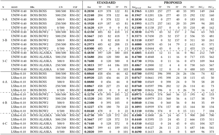
(7) Table 3: Classification results for standard RM+EC (without filters) and for the proposed method (with filters). Symbols and abbreviations have the same meaning as in Table 2. STANDARD N. 3-A. 3-B. 3-C. 4-A. 4-B. 4-C. ALGO. DBs. UNIW-0.40 UNIW-0.40 UNIW-0.40 UNIW-0.40 UNIW-0.40 UNIW-0.40 UNIW-0.40 UNIW-0.40 UNIW-0.40 UNIW-0.40 UNIW-0.40 UNIW-0.40 UNIW-0.40 UNIW-0.40 UNIW-0.40 LSBm-0.10 LSBm-0.10 LSBm-0.10 LSBm-0.10 LSBm-0.10 LSBm-0.10 LSBm-0.10 LSBm-0.10 LSBm-0.10 LSBm-0.10 LSBm-0.10 LSBm-0.10 LSBm-0.10 LSBm-0.10 LSBm-0.10. BOSS/BOSS BOSS/BOSS BOSS/BOSS BOSS/BOSS BOSS/BOSS BOSS/BOW2 BOSS/BOW2 BOSS/BOW2 BOSS/BOW2 BOSS/BOW2 BOSS/ALASKA BOSS/ALASKA BOSS/ALASKA BOSS/ALASKA BOSS/ALASKA BOSS/BOSS BOSS/BOSS BOSS/BOSS BOSS/BOSS BOSS/BOSS BOSS/BOW2 BOSS/BOW2 BOSS/BOW2 BOSS/BOW2 BOSS/BOW2 BOSS/ALASKA BOSS/ALASKA BOSS/ALASKA BOSS/ALASKA BOSS/ALASKA. PROPOSED. C/S. CLF. Err. TP. TN. FP. FN. Errpr ed. Err. TP. TN. FP. FN. INC. INCC. INCS. 500/500 500/250 500/0 250/500 0/500 500/500 500/250 500/0 250/500 0/500 500/500 500/250 500/0 250/500 0/500 500/500 500/250 500/0 250/500 0/500 500/500 500/250 500/0 250/500 0/500 500/500 500/250 500/0 250/500 0/500. RM+EC RM+EC RM+EC RM+EC RM+EC RM+EC RM+EC RM+EC RM+EC RM+EC RM+EC RM+EC RM+EC RM+EC RM+EC RM+EC RM+EC RM+EC RM+EC RM+EC RM+EC RM+EC RM+EC RM+EC RM+EC RM+EC RM+EC RM+EC RM+EC RM+EC. 0.2030 0.2240 0.2440 0.1920 0.1620 0.4330 0.5667 0.8360 0.2973 0.0300 0.4830 0.5680 0.7600 0.3853 0.2060 0.0860 0.0920 0.0880 0.0867 0.0840 0.1270 0.1520 0.2100 0.1227 0.0440 0.4730 0.5667 0.7440 0.3867 0.2020. 419 204 0 419 419 485 243 0 485 485 397 204 0 397 397 458 225 0 458 458 478 241 0 478 478 399 197 0 399 399. 378 378 378 187 0 82 82 82 42 0 120 120 120 64 0 456 456 456 227 0 395 395 395 180 0 128 128 128 61 0. 122 122 122 63 0 418 418 418 208 0 380 380 380 186 0 44 44 44 23 0 105 105 105 70 0 372 372 372 189 0. 81 46 0 81 81 15 7 0 15 15 103 46 0 103 103 42 25 0 42 42 22 9 0 22 22 101 53 0 101 101. 0.1965 0.1947 0.1830 0.1993 0.2100 0.3830 0.3573 0.3110 0.4080 0.4550 0.4805 0.4780 0.4730 0.4867 0.4880 0.0780 0.0767 0.0780 0.0760 0.0780 0.0975 0.0780 0.0840 0.1093 0.1110 0.4500 0.4440 0.4310 0.4580 0.4690. 0.1203 0.1201 0.1262 0.1175 0.1138 0.6795 0.7430 0.8307 0.5870 0.0444 0.4103 0.4848 0.5926 0.2000 0.0000 0.0592 0.0661 0.0569 0.0597 0.0616 0.0882 0.0979 0.1346 0.0939 0.0386 0.5000 0.5595 0.6522 0.4127 0.1613. 257 126 0 257 257 43 23 0 43 43 12 6 0 12 12 396 195 0 396 396 374 211 0 374 374 26 13 0 26 26. 277 277 277 141 0 32 32 32 14 0 11 11 11 4 0 398 398 398 202 0 360 360 360 157 0 24 24 24 11 0. 40 40 40 20 0 157 157 157 79 0 16 16 16 4 0 24 24 24 12 0 56 56 56 40 0 45 45 45 21 0. 33 15 0 33 33 2 2 0 2 2 0 0 0 0 0 26 18 0 26 26 15 6 0 15 15 5 2 0 5 5. 393 292 183 299 210 766 536 311 612 455 961 717 473 730 488 156 115 78 114 78 195 117 84 164 111 900 666 431 687 469. 149 132 101 94 48 63 55 50 41 13 212 155 109 163 103 74 65 58 41 16 42 38 35 30 7 200 155 104 146 96. 244 160 82 205 162 703 481 261 571 442 749 562 364 567 385 82 50 20 73 62 153 79 49 134 104 700 511 327 541 373. Table 4: Experiments with low bit rates. Symbols and abbreviations have the same meaning as in Table 2. STANDARD N. ALGO. DBs. 5. HILL-0.20 HILL-0.20 UNIW-0.20 UNIW-0.20. BOSS/BOSS BOSS/BOW2 BOSS/BOSS BOSS/BOW2. PROPOSED. C/S. CLF. Err. TP. TN. FP. FN. Errpr ed. Err. TP. TN. FP. FN. INC. INCC. INCS. 500/500 500/500 500/500 500/500. RM+EC RM+EC RM+EC RM+EC. 0.3530 0.4850 0.3360 0.4650. 350 474 352 485. 297 41 312 50. 203 459 188 450. 150 26 148 15. 0.3545 0.4875 0.3205 0.4620. 0.2509 0.7200 0.1922 0.5658. 106 4 145 19. 112 3 145 14. 36 15 34 40. 37 3 35 3. 709 975 641 924. 298 61 280 48. 411 914 361 876. Table 5: Experiments training with images from other databases. Symbols and abbreviations have the same meaning as in Table 2. STANDARD N. 6-A. 6-B. ALGO. DBs. HILL-0.40 HILL-0.40 HILL-0.40 HILL-0.40 HILL-0.40 HILL-0.40. BOWS2/BOWS2 BOWS2/BOSS BOWS2/ALASKA ALASKA/ALASKA ALASKA/BOSS ALASKA/BOWS2. PROPOSED. C/S. CLF. Err. TP. TN. FP. FN. Errpr ed. Err. TP. TN. FP. FN. INC. INCC. INCS. 500/500 500/500 500/500 500/500 500/500 500/500. RM+EC RM+EC RM+EC RM+EC RM+EC RM+EC. 0.2060 0.3140 0.4710 0.2950 0.4110 0.3710. 414 364 363 378 387 273. 380 322 166 327 202 356. 120 178 334 173 298 144. 86 136 137 122 113 227. 0.1900 0.3055 0.4685 0.2895 0.3905 0.3730. 0.1161 0.2031 0.3968 0.1354 0.2466 0.2756. 268 148 20 177 78 81. 280 162 18 187 87 103. 34 42 17 31 27 29. 38 37 8 26 27 41. 380 611 937 579 781 746. 148 259 277 236 201 439. 232 352 660 343 580 307. predicted classification error is correct, as far as the classifier is not working in these conditions, as evident from the balanced case (first row of Experiment 1-B). The reason why the classification error. is so small in the all-stego case is that the output of the classifier is stego for almost all images, which works by chance when all testing images are stego..
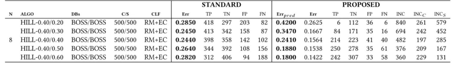
(8) Table 6: Experiments using the SRNet convolutional neural network. Symbols and abbreviations have the same meaning as in Table 2. STANDARD N. 7-A. 7-B. 7-C. ALGO. DBs. HILL-0.40 HILL-0.40 HILL-0.40 HILL-0.40 HILL-0.40 HILL-0.40 HILL-0.40 HILL-0.40 HILL-0.40. BOSS/BOSS BOSS/BOWS2 BOSS/ALASKA BOWS2/BOWS2 BOWS2/BOSS BOWS2/ALASKA ALASKA/ALASKA ALASKA/BOWS2 ALASKA/BOSS. PROPOSED. C/S. CLF. Err. TP. TN. FP. FN. Errpr ed. Err. TP. TN. FP. FN. INC. INCC. INCS. 500/500 500/500 500/500 500/500 500/500 500/500 500/500 500/500 500/500. SRNET SRNET SRNET SRNET SRNET SRNET SRNET SRNET SRNET. 0.2520 0.2600 0.3840 0.2670 0.3570 0.3880 0.3940 0.3930 0.3900. 434 447 441 437 452 319 324 438 386. 314 293 175 296 191 293 282 169 224. 186 207 325 204 309 207 218 331 276. 66 53 59 63 48 181 176 62 114. 0.2635 0.2855 0.3825 0.2720 0.3250 0.3805 0.3910 0.3930 0.4120. 0.1057 0.1235 0.2128 0.1272 0.2000 0.2218 0.2156 0.2150 0.2955. 216 178 75 184 156 80 76 77 68. 207 198 110 214 124 106 95 91 56. 35 33 22 35 62 28 34 35 43. 15 20 28 23 8 25 13 11 9. 527 571 765 544 650 761 782 786 824. 158 128 96 122 107 343 350 129 273. 369 443 669 422 543 418 432 657 551. Table 7: Experiments with unknown bitrate (SSM). Symbols and abbreviations have the same meaning as in Table 2. STANDARD N. ALGO. DBs. 8. HILL-0.40/0.20 HILL-0.40/0.30 HILL-0.40/0.40 HILL-0.40/0.50 HILL-0.40/0.60. BOSS/BOSS BOSS/BOSS BOSS/BOSS BOSS/BOSS BOSS/BOSS. PROPOSED. C/S. CLF. Err. TP. TN. FP. FN. Errpr ed. Err. TP. TN. FP. FN. INC. INCC. INCS. 500/500 500/500 500/500 500/500 500/500. RM+EC RM+EC RM+EC RM+EC RM+EC. 0.2850 0.2450 0.2440 0.2640 0.2820. 418 413 398 344 312. 297 342 358 392 406. 203 158 142 108 94. 82 87 102 156 188. 0.4200 0.3470 0.2410 0.1880 0.1800. 0.2625 0.1667 0.1564 0.1538 0.1422. 6 84 214 250 242. 112 171 223 278 307. 36 35 41 35 33. 6 16 40 61 58. 840 694 482 376 360. 261 242 197 209 229. 579 452 285 167 131. Note that Experiment 2 (Table 2) is the same as Experiment 1 (Table 2) but using 10,000 images for training and 10,000 images for testing. This experiment was carried out to check if the results with 1,000 images are stable enough. We can see that, in both cases, the results are very similar. In Experiments 3 and 4 (Table 3), the results obtained for the embedding algorithms UNIWARD and LSB matching are shown, and the accuracy of the predicted classification error is similar to that of Table 2. Comparable results are also obtained with low embedding bit rates, as it can be observed in Experiment 5 (Table 4) for the algorithms HILL and UNIWARD with 0.2 bpp. In the previous experiments, the database used for training is BOSS. In Experiment 6 (Table 5), we show the results obtained using images from other databases for training. More precisely, we use BOWS2 and ALASKA in the training set. As it can be observed, the results are comparable in terms of the accuracy of the prediction of the classification error. In Experiment 7 (Table 6), the results using the SRNet [3] classification method are presented, and different training databases are used. Again, the prediction of the classification errors is accurate. Experiment 8 (Table 7) presents the classification results in case of SSM. In this case, the testing set is embedded with HILL and 0.40 bpb, and the embedding bit rate of the training set varies between 0.20 and 0.60 bpp. When a wrong embedding bit rate is chosen, the prediction of the classification error is less accurate. The reason for this mismatch is that a wrong embedding rate is used to create the set B train and, hence, the classifier fˆB is not appropriate for the testing set. This problem will be addressed in our future work. Finally, in Experiments 9 and 10 (Table 8), we show the results obtained for JPEG images compressed to qualities 75 and 95, respectively. In this case, we have used the embedding algorithms UED. and J-UNIWARD, and the accuracy of the predicted classification error is consistent with that of the rest of the experiments. As shown in the experiments, the proposed method works both if there is CSM and when it is too difficult to classify images with the underlying classifier in case of a too small embedding bit rate.. 5. CONCLUSION. In this paper, a method for detecting inconsistencies in image steganalysis is presented. We show how the number of inconsistencies can be used to predict the classification error of the steganalytic method. The proposed approach has been tested for different steganalyzers, image databases, embedding algorithms and embedding bit rates, with and without CSM. The results show how the classification error of a steganalytic method can be predicted without having access to the labels of the images in the testing set. The predicted classification error can be a very valuable information for a steganalyst, who can decide how to proceed when the predicted classification error is too large. In such a case, increasing the training set in order to improve the classification accuracy could be one of the alternatives to be considered. The proposed method is intended to be used in batch steganography. Nevertheless, even for a single testing image, this approach makes it possible to detect if the classification is inconsistent. In such a case, the classifier should not be used to classify that image. As future work, it would be worth analyzing how to take profit of the proposed methodology when classifying single images. Finally, in case of stego source mismatch (e.g. when the embedding bit rate is not known accurately) the prediction of the classification is not reliable. Possible approaches to deal with this problem will be addressed in our future research..
(9) Table 8: Experiments with JPEG steganography. Symbols and abbreviations have the same meaning as in Table 2. STANDARD N. 9-A. 9-B. 9-C. 10-A. 10-B. 10-C. ALGO. DBs. UED-0.40 UED-0.40 UED-0.40 J-UNIW-0.40 J-UNIW-0.40 UED-0.40 UED-0.40 UED-0.40 J-UNIW-0.40 J-UNIW-0.40 UED-0.40 UED-0.40 UED-0.40 UED-0.40 UED-0.40 UED-0.40 J-UNIW-0.40 J-UNIW-0.40 UED-0.40 UED-0.40 UED-0.40 J-UNIW-0.40 J-UNIW-0.40 UED-0.40 UED-0.40 UED-0.40. BOSS-J75/BOSS-J75 BOSS-J75/BOWS2-J75 BOSS-J75/ALASKA-J75 BOSS-J75/BOSS-J75 BOSS-J75/BOWS2-J75 BOWS2-J75/BOWS2-J75 BOWS2-J75/BOSS-J75 BOWS2-J75/ALASKA-J75 BOWS2-J75/BOWS2-J75 BOWS2-J75/BOSS-J75 ALASKA-J75/ALASKA-J75 ALASKA-J75/BOSS-J75 ALASKA-J75/BOWS2-J75 BOSS-J95/BOSS-J95 BOSS-J95/BOWS2-J95 BOSS-J95/ALASKA-J95 BOSS-J95/BOSS-J95 BOSS-J95/BOWS2-J95 BOWS2-J95/BOWS2-J95 BOWS2-J95/BOSS-J95 BOWS2-J95/ALASKA-J95 BOWS2-J95/BOWS2-J95 BOWS2-J95/BOSS-J95 ALASKA-J95/ALASKA-J95 ALASKA-J95/BOSS-J95 ALASKA-J95/BOWS2-J95. PROPOSED. C/S. CLF. Err. TP. TN. FP. FN. Errpr ed. Err. TP. TN. FP. FN. INC. INCC. INCS. 500/500 500/500 500/500 500/500 500/500 500/500 500/500 500/500 500/500 500/500 500/500 500/500 500/500 500/500 500/500 500/500 500/500 500/500 500/500 500/500 500/500 500/500 500/500 500/500 500/500 500/500. GFR+EC GFR+EC GFR+EC GFR+EC GFR+EC GFR+EC GFR+EC GFR+EC GFR+EC GFR+EC GFR+EC GFR+EC GFR+EC GFR+EC GFR+EC GFR+EC GFR+EC GFR+EC GFR+EC GFR+EC GFR+EC GFR+EC GFR+EC GFR+EC GFR+EC GFR+EC. 0.0290 0.0300 0.2090 0.0820 0.1000 0.0240 0.0350 0.2070 0.0970 0.0960 0.0800 0.0680 0.0890 0.1530 0.1900 0.4310 0.2280 0.2640 0.1660 0.1690 0.4180 0.2600 0.2460 0.3040 0.2350 0.2400. 480 481 348 446 445 490 487 346 450 466 456 453 442 430 368 140 369 324 414 427 154 366 380 349 390 356. 491 489 443 472 455 486 478 447 453 438 464 479 469 417 442 429 403 412 420 404 428 374 374 347 375 404. 9 11 57 28 45 14 22 53 47 62 36 21 31 83 58 71 97 88 80 96 72 126 126 153 125 96. 20 19 152 54 55 10 13 154 50 34 44 47 58 70 132 360 131 176 86 73 346 134 120 151 110 144. 0.0315 0.0355 0.2315 0.0910 0.0990 0.0340 0.0305 0.2435 0.0990 0.1165 0.0955 0.0805 0.0925 0.1310 0.1635 0.4145 0.2295 0.2560 0.1525 0.1460 0.3995 0.2380 0.2380 0.2665 0.2065 0.2100. 0.0267 0.0215 0.1899 0.0819 0.0998 0.0193 0.0309 0.1910 0.0960 0.0769 0.0581 0.0536 0.0847 0.1220 0.1842 0.4152 0.2089 0.2295 0.1640 0.1427 0.3980 0.2481 0.2252 0.2227 0.2095 0.2224. 452 450 204 362 348 452 452 194 352 346 375 385 363 319 267 44 201 183 285 306 53 194 194 183 229 215. 460 459 231 389 374 462 458 221 373 362 387 409 383 329 282 56 227 193 296 301 68 200 212 180 235 236. 8 6 29 22 37 9 19 27 35 38 20 16 24 47 30 13 50 37 47 52 22 71 59 35 59 41. 17 14 73 45 43 9 10 71 42 21 27 29 45 43 94 58 63 75 67 49 58 59 59 69 64 88. 63 71 463 182 198 68 61 487 198 233 191 161 185 262 327 829 459 512 305 292 799 476 476 533 413 420. 34 35 291 92 93 25 23 309 88 89 94 88 99 115 198 675 244 320 143 127 648 249 223 249 186 224. 29 36 172 90 105 43 38 178 110 144 97 73 86 147 129 154 215 192 162 165 151 227 253 284 227 196. ACKNOWLEDGMENTS This work was supported by the Spanish Government, in part under Grant RTI2018-095094-B-C22 “CONSENT”, and in part under Grant TIN2014-57364-C2-2-R “SMARTGLACIS.” We gratefully acknowledge the support of NVIDIA Corporation with the donation of an NVIDIA TITAN Xp GPU card that has been used in this work.. REFERENCES [1] P. Bas, T. Filler, and T. Pevný. 2011. "Break Our Steganographic System": The Ins and Outs of Organizing BOSS. In Proceedings of the 13th International Conference on Information Hiding (IH’11). Springer-Verlag, 59–70. [2] P. Bas and T. Furon. [n. d.]. "Break Our Watermarking System 2nd. Ed.". http: //bows2.ec-lille.fr/. ([n. d.]). Accessed: July 2007. [3] M. Boroumand, M. Chen, and J. Fridrich. 2019. Deep Residual Network for Steganalysis of Digital Images. IEEE Transactions on Information Forensics and Security 14, 5 (May 2019), 1181–1193. [4] G. Cancelli, G. Doërr, M. Barni, and I. J. Cox. 2008. A Comparative Study of ±1 Steganalyzers. In Multimedia Signal Processing, 2008 IEEE 10th Workshop on. 791–796. [5] R. Cogranne and P. Bas. [n. d.]. "Alaska". https://alaska.utt.fr. ([n. d.]). Accessed: March 2019. [6] T. Denemark, V. Sedighi, V. Holub, R. Cogranne, and J. Fridrich. 2014. SelectionChannel-Aware Rich Model for Steganalysis of Digital Images. In 2014 IEEE International Workshop on Information Forensics and Security (WIFS). 48–53. [7] J. Fridrich and J. Kodovský. 2012. Rich Models for Steganalysis of Digital Images. IEEE Transactions on Information Forensics and Security 7 (2012), 868–882. [8] G. Gul and F. Kurugollu. 2011. A New Methodology in Steganalysis: Breaking Highly Undetectable Steganography (HUGO). In Proceedings of the 13th International Conference on Information Hiding. 71–84. [9] L. Guo, J. Ni, and Y. Q. Shi. 2014. Uniform Embedding for Efficient JPEG Steganography. IEEE Transactions on Information Forensics and Security 9, 5 (May 2014), 814–825. [10] V. Holub, J. Fridrich, and T. Denemark. 2014. Universal distortion function for steganography in an arbitrary domain. EURASIP Journal on Information Security 2014, 1 (2014), 1–13. [11] A. D. Ker. 2007. Batch Steganography and Pooled Steganalysis. In Proceedings of the 8th International Conference on Information Hiding (IH’06). Springer-Verlag,. Berlin, Heidelberg, 265–281. [12] A. D. Ker, P. Bas, R. Böhme, R. Cogranne, S. Craver, T. Filler, J. Fridrich, and T. Pevný. 2013. Moving Steganography and Steganalysis from the Laboratory into the Real World. In Proceedings of the First ACM Workshop on Information Hiding and Multimedia Security. 45–58. [13] J. Kodovský, J. Fridrich, and V. Holub. 2012. Ensemble Classifiers for Steganalysis of Digital Media. IEEE Transactions on Information Forensics and Security 7, 2 (2012), 432–444. [14] J. Kodovský, V. Sedighi, and J. Fridrich. 2014. Study of Cover Source Mismatch in Steganalysis and Ways to Mitigate its Impact. In Proceedings of SPIE - The International Society for Optical Engineering, Vol. 9028. [15] S. Kouider, M. Chaumont, and W. Puech. 2013. Adaptive steganography by oracle (ASO). In International Conference on Multimedia and Expo (ICME). IEEE, 1–6. [16] Daniel Lerch-Hostalot and David Megías. 2016. Unsupervised steganalysis based on artificial training sets. Engineering Applications of Artificial Intelligence 50 (2016), 45–59. [17] B. Li, M. Wang, J. Huang, and X. Li. 2014. A New Cost Function for Spatial Image Steganography. In 2014 IEEE International Conference on Image Processing (ICIP). 4206–4210. [18] I. Lubenko and A. D. Ker. 2012. Going from Small to Large Data in Steganalysis. In Media Watermarking, Security, and Forensics 2012 (Proceedings of SPIE - The International Society for Optical Engineering), Vol. 8303. 0M01–0M10. [19] J. Pasquet, S. Bringay, and M. Chaumont. 2014. Steganalysis with Cover-Source Mismatch and a Small Learning Database. In Proceedings of the 22nd European Signal Processing Conference (EUSIPCO). 2425–2429. [20] Tomás Pevný. 2011. Detecting Messages of Unknown Length. Proceedings of SPIE - The International Society for Optical Engineering 7880 (2011), 78800T–78800T–12. [21] T. Sharp. 2001. An Implementation of Key-Based Digital Signal Steganography. In Information Hiding. Lecture Notes in Computer Science, Vol. 2137. Springer, 13–26. [22] X. Song, F. Liu, C. Yang, X. Luo, and Y. Zhang. 2015. Steganalysis of Adaptive JPEG Steganography Using 2D Gabor Filters. In Proceedings of the 3rd ACM Workshop on Information Hiding and Multimedia Security (IH&MMSec ’15). 15–23. [23] X. Xu, J. Dong, W. Wang, and T. Tan. 2015. Robust Steganalysis based on Training Set Construction and Ensemble Classifiers Weighting. In 2015 IEEE International Conference on Image Processing (ICIP). 1498–1502..
(10)
Figure
+2

Documento similar