Universidad Nacional de La Plata
Sextas Jornadas de Economía
Monetaria e Internacional
La Plata, 10 y 11 de mayo de 2001
To Float or to Trail: Evidence on the Impact of Exchange Rate
Regimes
To Float or to Trail: Evidence on the Impact of
Exchange Rate Regimes
1Eduardo Levy-Yeyati
Business School, Universidad Torcuato Di Tella Miñones 2177 (1428) Buenos Aires – Argentina
Tel: 4783-3112 and 4787-9349 Fax: 4783-3220
e-mail: [email protected]
Federico Sturzenegger
Business School, Universidad Torcuato Di Tella Miñones 2177 (1428) Buenos Aires – Argentina
Tel: 4783-3112 and 4787-9349 Fax: 4783-3220
e-mail: [email protected]
January 2001
Abstract
We study the relationship between exchange rate regimes and economic growth for a sample of 154 countries over the post-Bretton Woods period (1974-1999), using a new de facto
classification of regimes based on the actual behavior of the relevant macroeconomic variables. In contrast with previous studies, we find that, for developing countries, less flexible exchange rate regimes are strongly associated with slower growth, as well as with greater output volatility. For industrial countries, on the contrary, regimes do not appear to have any significant impact on growth. The results are robust to endogeneity corrections and a number of alternative specifications borrowed from the growth literature.
1
1. INTRODUCTION
The choice of exchange rate regimes and its impact on economic variables is probably one of the most controversial topics in macroeconomic policy. However, while its implications regarding inflation and policy credibility have received considerable attention, the impact of regimes on economic growth has been the subject of surprisingly little work, probably due to the fact that nominal variables are typically considered to be unrelated to longer-term growth performance.2
Even when the economic literature does suggest a link between exchange rate regimes and growth, it does not provide unambiguous implications as to the sign of this link. On the one hand, the lack of exchange rate adjustments under a peg, coupled with some degree of short-run price rigidity, results in price distortions and misallocation of resources (notably, high unemployment) in the event of real shocks.3 This mechanism underscores the rather
uncontroversial view that fixed exchange rate regimes induce higher output volatility, a point further supported by the fact that, in a context of free capital mobility, fixed regimes entail the loss of monetary policy as an independent countercyclical mechanism.4 In addition, as
suggested by Calvo (1999) and others, the need to defend a peg in the event of a negative external shock implies a significant cost in terms of real interest rates, as well as increasing uncertainty as to the sustainability of the regime, potentially harming investment prospects. However, the implications of these channels in terms of long-run growth performance are less obvious.
On the other hand, by reducing relative price volatility, a peg is likely to stimulate investment and trade, thus increasing growth.5 Lower price uncertainty, usually associated with fixed exchange rate regimes, should also lead to lower real interest rates, adding to the same effect. Moreover, (credible) fixed exchange rate regimes are usually assumed to contribute to
monetary policy discipline and predictability, and to reduce a country’s vulnerability to speculative exchange rate fluctuations, all factors that are conducive to stronger growth performance.6
Thus, although the literature, if anything, seems to offer stronger arguments favoring the idea that fixed exchange rates may lead to higher growth rates, in the end, the question of whether or not there exists a link between regimes and growth can only be resolved as an empirical matter. The purpose of this paper is to address this issue by assessing the relationship between exchange rate regimes and output growth for a sample of 154 countries over the post Bretton
2
A notable exception is the inflation rate. See, e.g., De Gregorio (1993) and Roubini and Sala-i-Martin (1995), for theoretical models, and Levine and Renelt (1992), Barro (1995) and Andres et al. (1996) for an empirical exploration.
3
The view that flexible regimes are better suited to insulate the economy against real shocks go back to Friedman (1953) and Poole (1970), among others.
4
The view has found ample support in the empirical literature. See, e.g., Baxter and Stockman (1989), Mussa (1986), Broda (2000), Ghosh et al. (1997), and Bayoumi and Eichengreen (1994).
5
See, e.g., Frankel (1999), Rose (2000), Frankel and Rose (2000). Alternatively, Aizenman (1994) argues, in the context of a theoretical model, that higher output volatility as a result of the adoption of a peg may foster investment and growth.
6
Woods period (1974-1999). Contrary to what might have been inferred from the literature, we find that, for developing countries, less flexible exchange rate regimes are associated with slower growth. For industrial countries, on the contrary, we find that the regime type has no significant impact on growth. In addition, our tests confirm the standard view (and previous empirical work) indicating the presence of a negative link between output volatility and exchange rate flexibility. These results are robust to a number of alternative specifications and other checks.
Our main reference comes from the numerous empirical papers on the determinants of growth, from which we borrow our baseline specification.7 Also close to our work is the relatively scarce body of literature that directly addresses the relationship between growth and exchange rate regimes. Among the few papers within this group, Mundell (1995) looks at the growth performance for the industrial countries before and after the demise of Bretton Woods, finding that the former period was associated with faster average growth. On the other hand, Ghosh et al. (1997) run growth regressions controlling for the de jure exchange rate regimes as defined by the IMF, finding no systematic link between the two.8 We improve upon this work in two ways. First we use a de facto classification of exchange rate regimes that better captures the policies implemented by countries regardless of the regime reported by the country’s authorities.9 In addition, our model specification builds on existing results in the literature, focusing on the post-Bretton Woods period and expanding the sample size to include the 90s.
It is important to stress at this point that we do not intend to revisit previous findings in the growth literature nor to assess their sensitivity to various combinations of explanatory
variables or to the inclusion of exchange regime dummies. We draw on those findings only to obtain a reasonable set of additional controls to use as a benchmark to test whether the
exchange rate regime has a significant impact on growth. We find that, for the group of developing countries, this is indeed the case.
The paper proceeds as follows. Section 2 describes the data. Section 3 presents the baseline regressions. Section 4 details the results of selected robustness tests. Finally, section 5 discusses possible interpretations, and concludes.
2. THE DATA
Our sample covers annual observations for 154 countries over the period 1974-1999. A list of countries, as well as the definitions and sources of the variables used in the paper, is presented in Appendix 1. With the exception of the political instability and secondary enrollment
variables, all of our data comes from the IMF and the World Bank. Data availability varies across countries and periods, so that the tests in each subsection were run on a consistent subsample of observations (which is reported in each case along with the results).
7
See Levine and Renelt (1992), and Barro and Sala-I-Martin (1995), and references therein.
8
However, for some subsamples of countries they find weak evidence that growth rates in fixes are below those in floats. On the other hand, Ghosh et al. (2000) find that currency boards, which can be assimilated with hard pegs, tend to grow faster.
9
The classification of exchange rate regimes that we use in this paper deserves some comment. Most of the empirical literature on the evolution and implications of alternative exchange rate regimes groups countries according to a de jure classification based on the regime that
governments claim to have in place, as reported by the IMF in its International Financial Statistics. This approach, however, ignores the fact that many alleged floats intervene in the exchange market to reduce exchange rate volatility, while some fixers devalue periodically to accommodate independent monetary policies. To address this problem, we use a de facto
classification of exchange rate regimes, based on cluster analysis techniques, that groups countries according to the behavior of three variables closely related to exchange rate policy: i) Exchange rate volatility (σe), measured as the average of the absolute monthly percentage changes in the nominal exchange rate over the year; ii) Volatility of exchange rate changes
(σ∆e), measured as the standard deviation of the monthly percentage changes in the exchange
rate; and iii) Volatility of reserves (σr), measured as the average of the absolute monthly change in international reserves relative to the monetary base in the previous month.10
These variables are computed on an annual basis, so that each country-year observation represents a point in the (σe, σ∆e, σr) space. In this space, floats are associated with little
intervention in the exchange rate market together with high volatility of exchange rates. Conversely, observations with little volatility in the exchange rate variables coupled with substantial volatility in reserves correspond to the group of fixes. Finally, intermediate regimes are expected to exhibit moderate to high volatility across all variables, reflecting exchange rate movements in spite of active intervention. Thus, observations are grouped by proximity using cluster analysis according to the four clusters identified in Table 1.
Observations that do not display significant variability in either dimension are judged “inconclusives,” and left unclassified.11
TABLE 1
σ
σe σσ∆e∆ σσr
Flexible High High Low
Intermediate Medium Medium Medium
Fixed Low Low High
Inconclusive Low Low Low
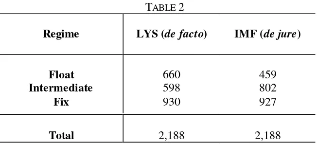
Table 2 shows the regime distribution of the 2188 classified observations, along with the alternative IMF-based classification for the same group of observations.
10
For a complete description of the classification methodology we refer the reader to Levy-Yeyati and Sturzenegger (2000). The three classifying variables are constructed based on IMF data. The database is available at http://www.utdt.edu/~ely or http://www.utdt.edu/~fsturzen .
11
TABLE 2
Regime LYS (de facto) IMF (de jure)
Float 660 459
Intermediate 598 802
Fix 930 927
Total 2,188 2,188
Source: IMF (de jure) from the International Financial Statistics. LYS (de facto), from Levy-Yeyati and Sturzenegger (2000).
While the two classifications show a similar number of fixed regimes, countries within this group differ substantially according to both classifications. This is due to the fact that de jure pegs that devalue regularly are classified as intermediates or floats, while countries that claim a flexible regime but intervene heavily to limit the fluctuations of the nominal exchange rate are typically classified as de facto fixers.
3. EXCHANGE RATE REGIMES AND GROWTH
A first pass at the data
Table 3 provides a first pass at the data, by showing the means and medians of the rate of growth of real per capita GDP (∆GDPPC) and its volatility (VOLGDPPC, measured as the standard deviation of the growth rate over a centered rolling five-year period). Observations are grouped by regime according to both the IMF and the de facto classifications. In addition, we show the corresponding statistics for industrial and developing countries.12 The table includes the 2041 observations (out of 2188 classified by the de facto methodology) for which growth data is available. Since the sample includes many countries which exhibit
extraordinary growth volatility (due to, for example, wars or transition to market economies) it seems more reasonable to concentrate the analysis in the medians which are less affected by such extreme values.
Simple inspection of the numbers anticipates the main results of the paper. Fixed exchange rates substantially underperform floating exchange rate regimes, under both classifications. In particular, the median annual real per capita growth rate drops from 2.2% for floaters to 1.6% for the group of pegs, according to the de facto classification. This difference is slightly narrower for the IMF classification. Note also that the difference in average growth, consistent with that of the medians when measured according to the de facto classification, has the opposite sign when based on the IMF. Thus, the de facto criterion appears to capture a more consistent connection between regimes and growth.13
12
Industrial and developing countries are listed in Appendix 1.
13
[image:6.612.137.463.74.222.2]The aggregate sample, however, masks important differences between industrial and developing countries. Whereas for the former there is basically no difference in growth performance across regimes, for developing countries the difference in the median growth rates widens to 0.8%.
As mentioned in the introduction, economic theory has long associated flexible regimes with smaller output volatility, as they insulate the economy from real shocks by adjusting exchange rates, allowing for relative price adjustments and reducing quantity (output) adjustments. This view has been documented by several empirical studies based on the IMF classification that find higher output volatility (and smaller real exchange rate volatility) in the case of currency pegs.14 As can be seen from Table 3, the de facto classification also indicates that output volatility decreases monotonically with the degree of flexibility of the exchange rate regime. Interestingly, much in the same way as in the case of growth, this link is entirely accounted for by the group of developing countries, while for industrial countries, once again, the regime appears to be irrelevant.
An alternative cut at the data is reported in Table 4. Here, we split countries into two groups, fast- and slow-growers, according to whether their average growth performance over the period 1974-1999 was below or above the median. We then examine whether any of these groups is characterized by adopting a particular exchange rate regime. To do that, we identify a country as fix (non-fix) whenever it is assigned a fixed (float or intermediate) regime in more than 50% of its available observations. We find that fixes account for 32% of the fast growers and 48% of the slow growers, again suggesting the presence of a negative link between pegs and growth. Once again, this link is entirely confined to the group of developing countries. Moreover, note that fast-growing developing countries are also characterized by smaller output volatility.
Growth regressions
We explore the robustness of our initial pass at the data by running a pooled regression for all country-year observations for which data is available. Since it is not our intention to
reexamine results profusely analyzed in the growth literature, we choose what we regard as a relatively non-controversial specification of the growth regression, to which we add the exchange rate regime dummies, INT and FIX.15
Regression results are presented in Table 5.16 As can be seen the control variables behave largely as expected. Real per capita growth (∆GDPPC) is positively correlated with both the investment-to-GDP ratio (INVGDP) and the rate of change of the terms of trade (∆TI),17 and negatively correlated with the growth of government consumption (GOV1, lagged to avoid potential endogeneity problems), population growth (POPGR), and political instability (CIVIL). Initial per capita GDP (GDPPC74, computed as the average over the period
14
See references in footnote 4.
15
Our baseline specifications follow closely those reported in Levine and Renelt (1992), which include the variables most frequently found in the empirical growth literature.
16
Standard errors reported in the table are corrected by heteroskedasticity, since a simple White-test rejected in all cases the null hypothesis of homoskedasticity.
17
1973) also comes out with a negative coefficient indicating the presence of conditional convergence. Secondary enrollment (SEC) and openness (OPEN) are not significant, in contrast with previous findings.18 In all cases, we include three regional dummies: Sub-Saharan Africa (SAFRICA), Latin America (LATAM) and transition economies (TRANS), as well as year dummies (the coefficients of which are omitted for conciseness).19
The coefficients of the regime dummies are consistent with the findings of the previous subsection. As a benchmark, we show in the first column the result of the test when regimes are assigned according to the IMF criterion: intermediate regimes grow significantly more than the rest with no difference between floaters and fixers.20
In contrast, the results based on the de facto classification reveal a different picture. The regression for the full sample indicates that growth rates are significantly higher for floaters than for less flexible regimes. Indeed, the coefficient of the fix dummy indicates that fixers grow on average close to 0.78% per year less than floaters.21 This suggests that, everything else equal, a country that opted for a flexible exchange rate after the demise of Bretton Woods would have ended up in 1999 with an output 21% larger than one that chose to fix.
A more careful analysis, however, reveals that the negative impact of pegs on growth is entirely accounted for by the group of non-industrial economies. In fact, for these countries, the coefficient of the fix dummy is larger in absolute value than for the general sample, indicating that the average growth rate of pegs is about 1% below that of floats. For industrial countries, on the other hand, neither of the dummies is statistically significant, once again suggesting that the exchange rate regime is irrelevant in these cases.
Output volatility
To explore the link between exchange rate regimes and output volatility, we run regressions exploiting the links suggested by the growth literature. The volatility of real per capita output growth (VOLGDPPC) is regressed against the volatilities of the investment ratio
(VOLINVGDP), of the change in government consumption (VOLGOV), and of the terms of trade (VOLTI), as well as measures of openness (OPEN), initial wealth (GDPPC74), and political instability (CIVIL). As before, we include regional and year dummies.
18
See, e.g., Barro and Sala - i – Martín (1995) and Edwards (1991). However, Levine and Renelt (1992) cast doubt on the robustness of these links.
19
It is important to emphasize at this point that the impact of exchange rate regimes reported in this paper proved to be robust to the inclusion of many other alternative controls suggested by the growth literature. These included the inflation rate, primary school enrollment, the ratio of exports and of imports to GDP, export and import growth, the GDP share of government consumption, the growth of domestic credit, the ratio of central government deficit to GDP, among others. The results, omitted here, are available from the authors upon request.
20
For the sake of comparison, the IMF regression includes only those observations that are also classified under the de facto methodology. Although we use a different sample, these results are comparable to those obtained in Ghosh et al. (1997), also based on the IMF classification.
21
The results are reported in Table 6. For the whole sample, the coefficients of all regressors are positive, indicating that higher volatility in macroeconomic fundamentals is associated with higher volatility of GDP. The growth of government consumption, terms of trade, the measure of civil liberties and two regional dummies are all significant.
The table also shows that, while fixed exchange rate regimes are associated with higher output volatility (as already documented in the literature), a more detailed analysis reveals that this association is, again, driven by non-industrial countries. As can be seen, the rest of the coefficients remains virtually unchanged when we move from the whole sample to the group of non-industrial countries, with the exception of the initial GDP level (GDPPC74), which coefficient doubles in value. This may be associated to the fact that the more financially developed emerging economies, which have been subject to considerable external shocks particularly during the nineties, correspond to the high income group among these countries.
Thus, in contrast with what the literature tells us, the evidence on the relationship between output volatility and exchange rate regimes is in fact rather mixed. More precisely, much in the same way as in the case of growth rates, the positive association between fixes and higher output volatility appears to be restricted to developing countries.
4. ROBUSTNESS
The volatility results discussed above, while mixed, were broadly consistent with the existing literature and empirical evidence. However, the growth results presented in the previous section, while also consistent with at least some of the hypothesis advanced in the literature (and discussed in the introduction), are nonetheless controversial. Thus, it is important to check the robustness of the growth results and their sensitivity to alternative specifications.
This section summarizes the various robustness checks that we run to address some of the potential concerns that our findings may give rise to. In particular, we discuss: a) cross-section regressions covering the whole period, to ensure that the link unveiled using annual data is not driven by short-term cyclical factors, b) the inclusion of additional macroeconomic variables to test for possible omitted variables, c) the distinction between high and low credibility pegs, and d) a correction for potential regime endogeneity.22 We address each of these checks in turn.
Cross section analysis
The basic motivation for our choice of frequency was the fact that regimes tend to change rather rapidly over time, making a longer-term regime classification less informative. However, there is an ample literature that stresses the short-run impact of changes in the
22
exchange rate regime on output performance.23 Thus, a potential criticism may arise from the fact that we use annual data to assess the impact on growth, possibly reflecting the short-term effect of a change in the exchange rate regime, rather than a long-term association between regimes and growth.
To address this concern, we estimate single cross section regressions à la Barro (1991), using averages of the relevant variables over the period 1974-1999, except for the variables
(GDPPC74 and SEC), which are measured at the start of the sample. The main difficulty posed by this exercise is the computation of the exchange rate regime dummy for those countries that changed their exchange rate policy during the period.
We test two alternative measures. First we use, for each country, the frequency with which it is classified as a fix (PERCFIX). Here, a value of 1 (0) would correspond to a country for which all available observations are classified as fix (float or intermediate). As an additional check, we use the simple average (LYSAVG) of a classification index that assumes the values 1, 2 or 3 whenever an observation is classified as float, intermediate or fix, respectively. In both cases, a negative coefficient would indicate a negative association between pegs and long-run growth.24
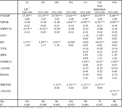
Table 7 presents the results of the single cross country regressions. To confirm that the
findings reported in the paper are not due to differences in the data, we start from a barebones specification that replicates Levine and Renelt’s (1992) “base” specification, and obtain comparable results despite the fact that we use a shorter sample period.25 Note also that, when the regime dummy is added to this basic set of regressors, it is still highly significant and of the expected sign.
We next take this “base” specification including the regime dummy, and expand the sample to include the 90s (column iv). As can be seen, with the exception of the investment ratio, the regressors are highly sensitive to the choice of period. Thus, both initial per capita GDP and secondary enrollment cease to be significant, while population growth, which was not significant in the previous sample, appears to be so now.26 In contrast, the regime dummy remains highly significant.
Finally, in column (v) and (vi), we go back to our baseline specification (similar to that of column (ii) in Table 5) but excluding in this case the annual change in terms of trade.27 As can be seen, countries that behaved more frequently as fixes displayed slower average growth
23
See, e.g., the extensive literature on exchange rate- vs. money-based stabilization as in Calvo and Vegh (1994a and b), Kiguel and Liviatan (1991) and Vegh (1992), to name just a few.
24
Note that the average measure LYSAVG is hampered by the fact that, as the results in Table 5 suggest, the relationship between regime flexibility and growth may not necessarily be monotonic.
25
Levine and Renelt’s (1992) “base” specification include those variables that are found in most empirical studies and that can thus be regarded as less controversial (denoted as I-variables in their paper). For the sake of comparison, in column (i) of Table 7 we reproduce Levine and Renelt’s results, reproduced from column (i) of Table 5 in their paper.
26
The sensitivity of traditional growth regressors to the choice of sample and the combination of explanatory variables has already been stressed in Levine and Renelt (1992).
27
rates over the period, a result that is entirely attributable to the sub-group of non-industrial countries.
For completeness, in column (vii) we report the results of the same regression when the regime proxy is computed as the simple average of the classification index for each particular country (LYSAVG), which, as can be seen, yields comparable results.28
High credibility pegs
The de facto methodology leaves unclassified a number of countries that display very little variability in both the nominal exchange rate and the stock or reserves. It could be argued that credible fixes are less likely to be tested by the market (hence exhibiting a lower volatility of reserves) and, possibly for the same reason, more likely to benefit from a stronger growth performance.29 If so, by leaving out the so-called “inconclusives” we would be ignoring this credibility dimension and discarding “good pegs,” thus biasing the results towards a negative association between fixed regimes and growth.
A natural way to address this concern is to include these “high credibility” pegs in our regressions. Since the de facto approach is silent as to the regime to be assigned to these observations, we simply classified as fixes all those de facto inconclusives that did not exhibit changes in their exchange rates, and we added them to our previous sample.30 The two
columns of Table 8 report the results of our baseline regression, this time using the expanded group of pegs. Column (i) shows that while, as expected, the negative impact of fixed
exchange rate regimes decreases somewhat in absolute value, the results remain basically unchanged. Alternatively, we include a new dummy (FIXINC) that takes the value of one whenever a fix was previously classified as inconclusive. The value of this term should capture any differential effect on growth corresponding to the presence of “high credibility” pegs. As shown in column (ii), this new dummy is not significant, suggesting that the distinction between low and high credibility pegs is not relevant.
Additional macroeconomic variables
It may be argued that countries with the worst economic fundamentals and policy track records are the ones most likely to adopt a peg, either in an attempt to gather some policy credibility or as a way to reduce the volatility that results from the lack of such credibility. We do not believe this to be a serious threat to our results, since they are robust to the inclusion of
28
Replacing PERCFIX by LYSAVG in the other regressions in the Table provides identical results, omitted here for brevity. Note that, because of the way in which these dummies are constructed, the size of their coefficients are not directly comparable with each other or with those in the previous sections.
29
This argument underlies the view that “hard pegs” (economies with a currency board or with no separate legal tender), are preferred to “soft pegs” (economies with conventional, adjustable, pegs). On this, see Fischer (2001), Calvo (2000b), Eichengreen and Haussman (1999). Ghosh et al. (2000) provides empirical evidence in favor of “hard pegs”.
30
nearly all the variables found to be relevant by the growth literature.31 Moreover, the use of a
de facto classification should dispel concerns about fixes faring worse than their more flexible counterparts due to the presence of currency or banking crises, since failed pegs are by
construction excluded from the fixed exchange rate group.
However, in order to address this potential omitted variable problem we conducted two
additional tests. First, to control for weak macroeconomic fundamentals, we included inflation (INF(-1), lagged to reduce potential endogeneity problems), and dummies for currency crises (CURR), and bank runs (BANK). The latter, taken from Frankel and Rose (1996) and Glick and Rose (1998), and Demirguc-Kunt and Detragiache (1998), respectively, assign a one to all countries and periods for which these authors identify a currency crash or an speculative attack, or a banking crisis.
As can be seen in column (i) of Table 9, all three variables are significant and of the expected negative sign. While the coefficients of the regime dummies are somewhat smaller in absolute value, the exchange rate regime remains a strongly significant determinant of growth
performance. This conclusion is further confirmed in column (iii), which presents the results of a similar test using cross section regressions, where we now included the average inflation for the period (INF).32
Second, we excluded de facto intermediate exchange rate regimes (column ii). Underlying this exercise is the hypothesis that slow growth within this group, which comprises countries with high exchange rate and reserve volatility, is likely to reflect, at least in part, a
deterioration of macroeconomic conditions. This is confirmed by the fact that the three additional macroeconomic variables included in this subsection lose explanatory power, with all but one becoming non-significant at a 90% level. However, the negative relation between pegs and growth rates is not affected by the exclusion of the intermediate group.
Dealing with endogeneity
The previous tests have documented a robust association between fixed exchange rate regimes and economic growth. However, one may still be worried about the possibility that our results may be reflecting reverse causation, that is, a relationship that goes from growth to the choice of exchange rate regime. We believe that this problem should be relatively minor for a
number of reasons. As we discussed above, the economic literature has not associated the choice of regime to growth performance, nor has it considered growth as a major determinant of the exchange rate regime.33
One can conceive the case in which the collapse of an unsustainable fixed regime gives way to the recovery of economic fundamentals and the resumption of growth. However, the empirical literature on financial crises has long linked poor growth with the occurrence of
31
See footnote 19.
32
The other variables are also averaged over the period. As before, the change in the terms of trade is excluded.
33
speculative attacks and currency and banking crisis,34 a channel that is likely to induce a
negative correlation between growth and exchange rate variability, thus going in the opposite direction of our results. On the other hand, the association between crises and output
contractions may indeed be behind the lower growth rates displayed by intermediates, if this group is capturing countries under financial distress. Correcting for endogeneity could
therefore strengthen the results for the fixed group while weakening them for the intermediate group.35
Similarly, (exchange rate-based) stabilizations that induced an output contraction in the short run may be contributing to create the negative correlation shown by our results. Again, however, the literature tends to argue in favor of the opposite effect, namely that exchange rate-based stabilizations has been largely expansionary in the short run.
At this point, it is important to stress that these short-run effects should disappear once we consider long-run averages as we did in the single cross section regressions above. This notwithstanding, our analysis would not be complete if we did not address potential
endogeneity problems. In order to do so, we use a feasible generalized two-stage IV estimator (2SIV) suggested by White (1984). White’s procedure not only provides the most efficient among all IV estimators, but also allows to correct simultaneously for heteroskedasticity, a problem that we found present in our baseline specification.36 The methodology requires finding instruments for the regime dummies, and implementing a two-stage procedure. Once consistent estimates of the error terms are obtained, they are used to compute the variance covariance matrix that allows to compute the estimator that maximizes efficiency while taking into account the potential heteroskedasticity problem.
In the first step, we estimate a standard multinomial logit model of the choice of exchange rate regime. To do that, we construct a regime index that takes the values 1, 2 or 3, according to whether the observation is classified as float, intermediate or fix, respectively, and run a multinomial logit regression on all the variables included in the growth regression, plus the following additional controls: the ratio of domestic credit over GDP (DCREDIT), the ratio of the country’s GDP over the US’s (SIZE), a measure of financial deepening (the ratio of quasimoney over narrow money, QMM), and the rate of growth of M2 (∆M2(-1), lagged to reduce potential endogeneity problems). Frankel and Rose (1996) show that DCREDIT is significantly and positively associated with the collapse of an exchange rate regime. The relative size variable is potentially related to the exchange rate regime by the usual argument that smaller countries tend to be more open and thus favor fixed exchange rate regimes. Other authors, notably Kaminsky and Reinhart (1999), have shown that the degree of financial deepening may be associated to the probability of a currency collapse, thus motivating the use of QMM as an instrument. Finally, an expansionary monetary policy is in principle at odds (and thus negatively correlated) with the choice of a fixed regime, which justifies the inclusion of lagged money growth in the first-stage equation.37
34
This literature, however, is relatively silent on causality. See Kaminsky and Reinhart (1999), Hardy and Pazarbazioglu (1998), Demirguc-Kunt and Detragiache (1998), Frankel and Rose (1996), Kaminsky et al. (1998), among many others.
35
As we will see below, this is exactly the case.
36
See footnote 16.
37
From the multinomial logit we obtain the predicted probabilities for an intermediate and a fixed regime (INTFIT, and FIXFIT, respectively) that we use as instruments for the regime dummies in our baseline specification of the growth regression. This provides the consistent estimates of the error terms from which we compute the White’s efficient covariance matrix and 2SIV estimator.38 The results are presented in the first column of Table 10. As the table shows, the negative association between fixed regimes and growth is robust to the correction for endogeneity. Indeed, as was expected from the above discussion, the correction increases the negative impact of pegs on growth, raising the coefficient from 0.8% (see column (ii) of Table 5) to about 2%, significant at the P = 5.7% level. The dummy for intermediates, on the other hand, is no longer significant, supporting the view that the original result for the case of intermediate regimes may have reflected the impact of growth on the probability of a collapse of the regime, as already explored by Frankel and Rose (1996). The second column of Table 10 includes an alternative model in which we use as second-stage instruments the exogenous variables used in the first stage (DCREDIT, QMM, SIZE, ∆M2(-1)), in addition to INTFIT and
FIXFIT. As can be seen the results remain basically unchanged.
In order to obtain a cleaner test of the impact of pegs, we repeat the same procedure this time excluding intermediates from the sample, and computing a new first-stage estimate (FIXFIT2) from a binomial (instead of a multinomial) logit model and the same set of controls. The results, presented in columns (iii) and (iv) of Table 10, show that the coefficient remains virtually unchanged, and highly significant.
In conclusion, regardless of whether growth performance is itself a determinant of the choice of the exchange rate regime, the evidence indicates the presence of a strong independent link which goes from the choice of a peg to sluggish growth.
5. CONCLUSION
This paper tried to provide evidence on the implications of the choice of a particular exchange rate regime on economic growth. In contrast with previous findings, ours strongly suggest that exchange rate regimes indeed matter in terms of real economic performance for non-industrial countries, while this link appears to be much weaker for industrial economies. In particular, we found that, for the former, fixed exchange rate regimes are connected with slower growth rates and higher output volatility, an association that proved to be robust to several alternative specifications and checks.
While we have not specifically tested the hypothesis supporting the existence of a positive link between fixed exchange rates and trade surveyed in Frankel (1999), it is clear that whatever beneficial influence this might have on growth is not sufficient to generate a net positive impact of pegging on economic growth. Similarly, the alleged gains in terms of policy stability and predictability frequently attributed to fixed regimes, if present, are at odds with the higher output volatility that characterizes them.
Of the two arguments mentioned in the introduction that point to a negative effect of fixing, the idea that pegs may be subject to costly speculative attacks relates to Calvo (1999), who
38
claims that the external shocks suffered by a country are not unrelated to their exchange rate regime. According to this view, countries that fix the exchange rate are exposed to larger and more frequent shocks. Thus, the fixed exchange rate dummy may be capturing the effect of having these additional shocks, much in the same way that the political variables in the traditional growth equations also capture the implications of additional instability. Two points, however, cast doubt on this potential interpretation of our results. On the one hand, these additional shocks were to some extent tested in our regressions by controlling for the occurrence of currency and banking crises. In fact, while these variables were found to be significant, their inclusion reduced the size and significance of the regime dummy only marginally. On the other hand, “high credibility” pegs, which are not subject to frequent external shocks, did not appear to fare better in terms of growth than their more vulnerable counterparts.
An alternative hypothesis is the one that points at a combination of fixed exchange rate regimes and downward price rigidity that, in turn, may induce an asymmetric response to real shocks, in the form of output contractions when they are negative and price adjustment when they are positive. A careful examination of this channel may help understand the links
unveiled in this paper.39
As it stands, the paper opens more questions than it answers. If we accept the results reported here, one can only wonder why countries have opted so pervasively for unilateral pegs. At this point, however, one should be cautious not to read in our results the policy implication that countries should massively adopt floating exchange rate regimes. Fixed exchange rates may in some cases report substantial gains in terms of credibility and inflation performance,
particularly in a high inflation context. Additionally, the costs of the transition to a float are not minor and depend heavily on initial conditions. For example, for countries with
widespread financial dollarization, a move to a flexible regime may increase output volatility due to the balance sheet effect of fluctuations in the nominal exchange rate. Similarly, our findings are not incompatible with the advocacy of “hard pegs” or full dollarization. Many of the benefits of having a common currency or undertaking outright dollarization are not shared by unilateral pegs, transaction costs being just one example. Thus, as much as our results cast a negative light on fixed exchange rates, they leave open the debate regarding the tradeoff between hard pegs and fully floating regimes.
39
REFERENCES
Aizenman, Joshua (1994) Monetary and Real Shocks, Productive Capacity and Exchange Rate Regimes, Economica, Vol. 61, pp. 407/434.
Andrés, Javier, Ignacio Hernando and Malte Kruger (1996) Growth, Inflation and the Exchange Rate Regime, Economic Letters 53, pp. 61-65.
Barro, Robert (1995) Inflation and Economic Growth, Bank of England Quarterly Bulletin, May, pp. 1-11.
Barro, Robert (1991) Economic Growth in a Cross Section of Countries. Quarterly Journal of Economics, May, pp. 407-443.
Barro, Robert and Xavier Sala-I-Martin (1995) Economic Growth, McGraw Hill.
Baxter, Marianne and Stockman, Alan (1989) Business Cycles and the Exchange-Rate Regime: Some International Evidence, Journal of Monetary Economics, No. 23, pp.377-400.
Bayoumi, T. and Eichengreen, Barry (1994) Economic Performance under Alternative Exchange Rate Regimes: Some Historical Evidence, in The International Monetary System, ed by Kenen, Peter; Papaida, Francesco; and Saccomanni Fabrizzio. Cambridge University Press, pp. 257-297.
Broda, Christian (2000) Terms of Trade and Exchange Rate Regimes in Developing Countries, mimeo Massachusetts Institute of Technology.
Calvo, Guillermo (1999) Fixed versus Flexible Exchange Rates: Preliminaries of a Turn-of-Millennium Rematch, mimeo University of Maryland.
Calvo Guillermo (2000a) Testimony on Dollarization, mimeo University of Maryland.
Calvo Guillermo (2000b) The Case for Hard Pegs in the Brave New World of Global Finance,
mimeo University of Maryland.
Calvo, Guillermo and Carlos Vegh (1994a) Credibility and the dynamics of stabilization policy: a basic framework, in Advances in Econometrics: Sixth World Congress, Volume II, edited by Christopher Sims, Cambridge University Press, pp. 377-420.
Calvo, Guillermo and Carlos Vegh (1994b) Inflation Stabilization and Nominal Anchors,
Contemporary Economic Policy, Vol. XII, April, pp. 35-45.
De Gregorio, José (1993) Inflation, Taxation and Long-Run Growth, Journal of Monetary Economics, No. 31, pp.271-298.
Demirguc-Kunt and Detragiache (1998) Financial Liberlization and Financial Fragility, IMF Working Paper, WP/98/83.
Dornbusch, Rudiger (2000) Fewer Monies, Better Monies, Mimeo, MIT. December.
Edwards, Sebastian (1996) The Determinants of the Choice Between Fixed and Flexible Exchange–Rate Regimes, NBER Working Paper No. 5756.
Eichengreen, Barry and Ricardo Haussman (1999) Exchange Rates and Financial Fragility,
NBER Working Paper No. 7418.
Fischer, Stanley (2001), "Exchange Rate Regimes: Is the Bipolar View Correct?,"
Distinguished Lecture on Economics in Government, delivered at the AEA meetings in New Orleans on January 6, 2001
Frankel, Jeffrey (1999) No single Currency Regime is Right for all Countries or at all Times,
NBER Working Paper No. 7338.
Frankel, Jeffrey and Andrew Rose (1996) Currency Crisis in Emerging Markets: Empirical Indicators, NBER Working Paper No. 5437.
Frankel, Jeffrey and Andrew Rose (2000) Estimating the Effect of Currency Unions on Trade and Output, NBER Working Paper No. 7857.
Friedman, Milton (1953) The Case For Flexible Exchange Rates, in Essays in Positive Economics, University of Chicago Press.
Ghosh, Atish, Anne-Marie Gulde and Holger Wolf (2000) Currency Boards: More than a Quick Fix?, Economic Policy 31, October, pp. 270-335.
Ghosh, Atish, Anne-Marie Gulde, Jonathan Ostry and Holger Wolf (1997) Does the Nominal Exchange Rate Matter? NBER Working Paper No. 5874.
Glick, Reuven and Andrew Rose (1998), Contagion and Trade, Why are Currency Crises Regional? NBER Working Paper, No. 6806, November.
Hardy and Pazarbazioglu (1999) Determinants and Leading Indicators of Banking Crises, by Daniel C. Hardy and Ceyla Pazarbasioglu, IMF Staff Papers, Vol. 46, No. 3.
Kaminsky, Graciela and Carmen Reinhart (1999) The Twin Crises: The Causes of Banking and Balance-of-Payments Problems, American Economic Review, Vol. 89, No. 3.
Kaminsky, Graciela; Lizondo, Saul and Reinhart, Carmen (1998) Leading Indicators of Currency Crisis, IMF Staff Papers, Vol. 45, No. 1.
Kiguel, Miguel and Nissan Liviatan (1991) The Inflation Satbilization Cycles in Argentina and Brazil, in Lessons of Economic Stabilization and Its Aftermath, ed. by Michael Bruno and Stanley Fischer. MIT Press.
Levine, Ross and Renelt, David (1992) A Sensitivity Analysis of Cross-Country Growth Regressions. American Economic Review, Vol. 82, no. 4, pp. 942-963.
Maddala, G. (1989) Limited Dependent and Qualitative Variables in Econometrics, Cambridge: Cambridge University Press.
Mundell, Robert (1995) Exchange Rate Systems and Economic Growth, Rivista de Politica Economica, Vol. 85, No. 6, pp. 1-36.
Mussa, Michael (1986) Nominal Exchange Rate Regimes and the Behavior of Real Exchange Rates, Evidence and Implications, in Real Business Cycles, Real
Exchange Rates, and Actual Policies, ed. by Karl Brunner and Alan Meltzer, North-Holland Press.
Poole, William (1970) Optimal Choice of Monetary Policy Instruments in a Simple Stochastic Macro Model, Quarterly Journal of Economics, No. 84, pp. 197-216.
Roubini, Nouriel and Xavier Sala-I-Martin (1995) A Growth Model of Inflation, Tax Evasion, and Financial Repression, Journal of Monetary Economics, No. 35, pp.275-301.
Rose, Andrew (2000) One Money, One Market? The Effects of Common Currencies on International Trade. Economic Policy.
Vegh, Carlos (1992) Stopping High Inflation: An Analytical Overview, IMF Staff Papers, Vol. 39, pp. 626-695.
APPENDIX 1
(a) Variables and Sources
Variable Definitions and sources
∆GDPPC Rate of growth of real per capita GDP (Source: World Economic Outlook [WEO])
∆M2 (-1) Rate of growth of M2 (lagged one period) (Source: IMF)
∆TI Change in terms of trade - exports as a capacity to import (constant LCU) (Source: WDI; variable NY.EXP.CAPM.KN)
BANK Banking crises (Source: Demirguc-Kunt and Detragiache [1998])
CIVIL Index of civil liberties (measured on a 1 to 7 scale, with one corresponding to highest degree of freedom) (Source: Freedom in the World - Annual survey of freedom country ratings)
CURR Currency crashes (Source: Frankel and Rose [1996, 2000])
DCREDIT Net domestic credit (current LCU) (Source: WDI, variable FM.AST.DOMS.CN). GDPPC74 Initial per capita GDP (average over 1970-1973) (Source: WEO)
GOV1 Growth of government consumption (lagged one period) (Source: IMF) INF Annual percentage change in Consumer Price Index (Source: IMF).
INF (-1) Annual percentage change in Consumer Price Index (lagged one period) (Source: IMF).
INVGDP Investment to GDP ratio (Source: IMF’s International Financial Statistics [IMF]) LATAM Dummy variable for Latin American countries
OPEN Openness, (ratio of [export + import]/2 to GDP) (Source: IMF).
POPGR Population growth (annual %) (Source: World Development Indicators [WDI], variable SP.POP.GROW)
QMM Ratio quasimoney/money (Source: IMF)
SAFRICA Dummy variable for sub-Saharan African countries
SEC Total gross enrollment ratio for secondary education (Source: Barro [1991]) SIZE GDP in dollars over US GDP (Source: IMF).
TRANS Dummy variable for Transition economies
VOLGDPPC Standard deviation of the growth rate over a centered rolling five-year period
VOLGOV Standard deviation of the growth of government consumption over a centered rolling five-year period
VOLINVGDP Standard deviation of the investment to GDP ratio over a centered rolling five-year period
(b) List of Countries (154-country sample)
Australia (I) Cambodia Jordan Qatar
Austria (I) Cameroon Kazakhstan Romania Belgium (I) Central African Republic Kenya Russia
Canada (I) Colombia Korea Rwanda
Denmark (I) Comoros Kyrgyz Republic Saint Kitts and Nevis Finland (I) Congo Lao People's Dem.Rep Saint Lucia
France (I) Costa Rica Latvia Saint Vincent
Germany (I) Côte d'Ivoire Lebanon Sao Tome & Principe
Greece (I) Croatia Lesotho Saudi Arabia
Iceland (I) Cyprus Libya Senegal
Ireland (I) Czech Republic Lithuania Seychelles
Italy (I) Chad Luxembourg Sierra Leone
Japan (I) Chile Macedonia, Fyr Singapore Netherlands (I) Djibouti Madagascar Slovak Republic New Zealand (I) Dominica Malawi Slovenia
Norway (I) Dominican Republic Malaysia South Africa Portugal (I) Ecuador Maldives Sri Lanka
Spain (I) Egypt Mali Sudan
Sweden (I) El Salvador Mauritania Suriname Switzerland (I) Equatorial Guinea Mauritius Swaziland
United Kingdom (I) Estonia Mexico Syrian Arab Republic United States (I) Ethiopia Moldova Tanzania
Albania Gabon Mongolia Thailand
Antigua and Barbuda Gambia Morocco Togo
Argentina Georgia Mozambique Tonga
Armenia Ghana Myanmar Trinidad and Tobago
Azerbaijan Grenada Namibia Tunisia
Bahamas, The Guatemala Nepal Turkey
Bahrain Guinea Netherlands Antilles Uganda Bangladesh Guinea-Bissau Nicaragua Ukraine
Barbados Guyana Niger United Arab Emirates
Belize Haiti Nigeria Uruguay
Benin Honduras Oman Venezuela
Bhutan Hong Kong Pakistan Yemen
Bolivia India Papua New Guinea Zaire
Brazil Indonesia Paraguay Zambia
Bulgaria Iran Peru Zimbabwe
Burkina Faso Israel Philippines
Burundi Jamaica Poland
APPENDIX 2
White’s efficient 2SIV estimates
The estimation in Table 10 shows the results corresponding to White’s (White, 1984) efficient
2SIV (two-stage instrumental variable) estimator. This procedure delivers the asymptotically
efficient estimator among the class of IV estimators, even in the presence of a nonspherical
variance covariance matrix (VCV) for the error term in the structural equation. Consider the
structural equation for variable i:
i i i
i X
y = δ +ε ,
where the matrix X includes both endogenous and exogenous variables. In our specification yi
corresponds to the real per capita GDP growth rate and X includes both the exogenous
regressors in the growth equation as well as the endogenous regime dummy. The White
heteroskedasticity test mentioned in footnote 16 suggests that the VCV matrix of ε is
non-spherical, i.e.
Ω =
) ( i
V ε .
As is well known we can estimate consistently our parameter of interest, δ, by finding the
value of δ that minimizes the quadratic distance from zero of Z’(y-Xδ), i.e.
) (
' )' (
min
ˆ δ δ
δ
δ y−X ZRZ y−X
where Z indicates a set of instrumental variables. R corresponds to any symmetric positive
definite matrix, which must be chosen appropriately, however, in order to achieve asymptotic
efficiency. The estimator corresponding to the minimization problem is:
y ZRZ X X ZRZ
X' ' ) ' ' (
ˆ= −1
δ . (1)
It can be shown the limiting distribution of δˆ is
]) ) ' )( ' ( ) ' lim[( , 0 ( ) ˆ
( − ≈ −1 −1
RQ Q RVRQ Q RQ Q p N
T δ δ ,
where ) ' var( ' lim 2 / 1 ε Z T V T X Z p Q − = = (2)
Proposition 4.45 in White (1984) proves that choosing R = V-1 provides the asymptotically
efficient IV estimator. In this case, the distribution of the estimator is
) ) ' lim( , 0 ( ) ˆ
( − ≈ N p QV−1Q −1
T δ δ . (3)
Thus, if we choose R to obtain the asymptotically efficient estimator, we need an estimator of
V. However, because the ε’s are not observable, we need consistent estimators of the errors in
order to construct a feasible estimator for the VCV. Thus the procedure is as follows. We first
regime dummies, our endogenous variables. This multinomial (binomial) logit equation
includes the exogenous variables in the original structural equation plus the additional
exogenous variables discussed in the text, which are correlated with the choice of regime. The
estimated probabilities of the regimes are used as an instrument of the regime dummies in the
original specification.40 This simple IV estimator is used to obtain a consistent estimate for
the ε’s, which are then used to estimate is a consistent estimate of V, Vˆ , as:
T z z V t
t t t
∑
=
2 ˆ ' ˆ
ε
,
which allows for heteroskedasticity. Using Vˆ we can implement the estimator δˆ as in (1) and
compute its VCV matrix as in (3).
40
22 TABLE 3. RATE AND VOLATILITY OF REAL PER CAPITA GDP GROWTH (% PER YEAR)
IMF LYS Industrials Non-Industrials
FLOAT INT FIX FLOAT INT FIX FLOAT INT FIX FLOAT INT FIX
Observations 409 749 883 615 562 864 202 104 120 413 458 744
DGDPPC Means 1.0 2.0 1.2 1.9 0.8 1.5 1.9 1.6 2.3 1.9 0.6 1.4
Medians 1.7 2.3 1.2 2.2 1.4 1.6 2.3 1.8 2.1 2.1 1.1 1.3
VOLGDPPC Means 4.1 3.2 5.0 3.5 4.0 4.8 2.2 1.8 1.9 4.1 4.4 5.2
Medians 2.4 2.2 3.9 2.3 3.0 3.6 1.8 1.8 1.6 2.8 3.6 4.0
Source: IMF’s International Financial Statistics
TABLE 4. FAST AND SLOW GROWERS
Full Sample FAST
GROWERS
SLOW
GROWERS
P-value
Observations 77 77
DGDPPC Means 3.23 -0.34
Medians 2.59 -0.07
PERCFIX Means 0.32 0.48 0.049 1
VOLGDPPC Means 3.91 4.57 0.141 1
Medians 3.16 4.32 0.003 2 Mean growth rate (whole sample): 1.45
Industrials FAST
GROWERS
SLOW
GROWERS
P-value
Observations 11 11
DGDPPC Means 2.63 1.38
Medians 2.34 1.66
PERCFIX Means 0.36 0.27 0.666 1
VOLGDPPC Means 2.05 1.97 0.752 1
Medians 1.85 1.99 0.896 2 Mean growth rate (whole sample): 2.01
Non-Industrials FAST
GROWERS
SLOW
GROWERS
P-value
Observations 66 66
DGDPPC Means 3.31 -0.60
Medians 2.66 -0.16
PERCFIX Means 0.30 0.53 0.008 1
VOLGDPPC Means 4.32 4.86 0.269 1
Medians 3.42 4.50 0.017 2 Mean growth rate (whole sample): 1.35
1 corresponds to a t-test of equality of means
TABLE 5. GROWTH REGRESSIONS (ANNUAL DATA)
(i ) (ii ) (iii ) (iv )
IMF Baseline
LYS Baseline
LYS Industrial
LYS Non-industrial
INVGDP 9.26*** 8.67*** 7.28** 10.34***
1.89 1.88 3.03 2.45
POPGR -0.40** -0.46*** -0.69** -0.43**
0.16 0.15 0.32 0.17
GDPPC74 -0.34*** -0.38*** -0.24** -0.53*
0.13 0.12 0.11 0.28
GOV1 -1.27*** -1.13*** 2.95 -1.23***
0.40 0.40 2.07 0.42
SEC -0.65 -0.71 2.72** 0.20
0.97 0.95 1.35 1.32
CIVIL -0.24* -0.26** -0.57** -0.24*
0.12 0.12 0.23 0.14
∆TI 5.15*** 5.21*** 6.16** 5.27***
1.02 1.02 2.46 1.02
OPEN -0.61 -0.13 0.74 -1.30
0.81 0.82 0.93 0.82
SAFRICA -0.76* -0.94** -0.78
0.45 0.46 0.49
LATAM -0.93*** -0.96*** -0.97***
0.34 0.34 0.36
TRANS -0.90 -1.59 -2.17
1.85 1.74 1.79
INT 0.68** -0.98*** -0.43 -1.17***
0.29 0.29 0.28 0.38
FIX -0.16 -0.78*** -0.06 -1.04***
0.41 0.28 0.30 0.40
Obs. 1349 1349 387 962
R2 0.201 0.203 0.382 0.200
TABLE 6. OUTPUT VOLATILITY REGRESSIONS (ANNUAL DATA)
(i) (ii ) (iii )
Whole sample Industrials Non-industrials
GDPPC74 0.18** 0.10 0.42***
0.08 0.10 0.14
VOLINVGDP 0.09 14.63 -1.14
3.44 9.17 3.61
VOLGOV 1.7*** 16.03** 1.68***
0.61 6.25 0.59
VOLTI 0.01* -0.07 0.01
0.004 0.55 0.004
OPEN 1.69*** 1.58*** 1.35**
0.49 0.57 0.56
CIVIL 0.57*** 0.17 0.51***
0.09 0.22 0.11
SAFRICA 0.31 0.28
0.36 0.38
LATAM 0.69*** 0.43
0.21 0.29
TRANS 1.91*** 1.3**
0.56 0.63
INT 0.15 -0.49** 0.26
0.29 0.21 0.34
FIX 0.57** 0.03 0.71**
0.26 0.24 0.32
Obs. 1091 140 951
R2 0.141 0.618 0.113
TABLE 7. SINGLE CROSS SECTION GROWTH REGRESSIONS
(i) (ii) (iii) (iv) (v) (vi) (vii)
LR 1
1960-1989 1974-1989 1974-1989 1974-1999 1974-1999
Non Industrials
1974-1999 1974-1999 INVGDP 17.49** 14.15*** 15.78*** 13.61*** 8.80*** 10.19*** 8.46***
2.68 3.03 3.01 2.46 2.97 3.42 2.96
POPGR -0.38 -0.28 -0.28 -0.64*** -0.59*** -0.70*** -0.60***
0.22 0.24 0.23 0.14 0.18 0.21 0.18
GDPPC74 -0.35** -0.42** -0.39* -0.08 -0.23 -0.06 -0.24
0.14 0.20 0.20 0.14 0.16 0.24 0.16
GOV1 -1.16 -1.59* -0.91
0.84 0.91 0.82
SEC 3.17** 3.20*** 2.43** -0.005 -0.02 -0.03** -0.02
1.29 1.17 1.18 0.01 0.01 0.01 0.01
CIVIL -0.14 -0.05 -0.14
0.19 0.21 0.19
OPEN 1.05 1.25 1.30
0.99 1.31 1.02
SAFRICA -1.02** -0.91* -1.04**
0.48 0.52 0.47
LATAM -0.73 -0.55 -0.74*
0.44 0.52 0.44
TRANS -0.39 0.01 -0.72
1.41 1.56 1.41
PERCFIX -1.12** -1.33*** -1.31*** -2.27***
0.44 0.42 0.47 0.64
LYSAVG -0.77***
0.27
Obs. 101 86 86 101 96 74 96
R2 0.46 0.398 0.441 0.425 0.481 0.547 0.481
***, **, and * represent 99, 95 and 90% significance. Standard errors in italics.
1
TABLE 8. INCLUDING HIGH CREDIBILITY PEGS
(i) (ii )
Are high Credibility Pegs Different?
INVGDP 9.78*** 9.77***
1.73 1.73
POPGR -0.48*** -0.48***
0.15 0.15
GDPPC74 -0.47*** -0.47***
0.14 0.14
GOV1 -1.15*** -1.14***
0.39 0.39
SEC 0.06 0.07
0.97 0.97
CIVIL -0.16 -0.16
0.11 0.11
∆TI 5.42*** 5.43***
0.94 0.94
OPEN -1.00 -0.97
0.80 0.82
SAFRICA -1.24*** -1.23***
0.42 0.42
LATAM -0.89*** -0.89***
0.30 0.30
TRANS -1.70 -1.70
1.72 1.72
INT -0.93*** -0.93***
0.29 0.29
FIX -0.59** -0.62**
0.25 0.27
FIXINC 0.08
0.39
Obs. 1572 1572
R2 0.204 0.204
TABLE 9. INCLUDING ADDITIONAL MACROECONOMIC VARIABLES
(i) (ii) (iii)
Baseline specification
Baseline specification w/o intermediates
Single cross section 1
INVGDP 8.10*** 5.25** 9.13**
1.94 2.04 3.48
POPGR -0.36*** -0.33** -0.59***
0.13 0.13 0.20
GDPPC74 -0.26** -0.08 -0.11
0.11 0.12 0.18
GOV1 0.30 -0.32 3.69*
0.77 1.23 2.21
SEC -0.57 -0.91 -0.02
0.94 1.13 0.01
CIVIL -0.15 -0.12 -0.12
0.13 0.15 0.19
∆TI 4.87*** 5.02***
1.09 1.32
OPEN 0.11 1.19 0.87
0.80 0.92 0.93
INF(-1) -0.02* 0.002
0.01 0.010
INF -0.04**
0.02
CURR -1.75*** -2.08** 2.42
0.55 0.87 3.20
BANK -1.12** -0.10 -1.17
0.44 0.47 1.12
SAFRICA -1.21*** -0.86* -0.70
0.46 0.48 0.53
LATAM -0.77** -0.91** -0.71
0.35 0.39 0.49
TRANS -1.01 0.46 -0.96*
1.78 1.33 0.55
INT -0.85***
0.26
FIX -0.57** -0.64**
0.28 0.28
PERCFIX -1.39***
0.49
Obs. 1268 876 95
R2 0.217 0.182 0.489
TABLE 10. ACCOUNTING FOR ENDOGENEITY
(i) Baseline specification
(ii) Baseline specification
(iii)
Baseline specification w/o Intermediates
(iv)
Baseline specification w/o intermediates
INVGDP 8.58*** 8.71*** 3.96** 3.35*
2.00 2.07 1.99 1.99
POPGR -0.47*** -0.47*** -0.53*** -0.50***
0.16 0.13 0.17 0.17
GDPPC74 -0.40** -0.30** -0.10 -0.10
0.16 0.15 0.20 0.20
GOV1 -1.29*** -0.98*** -0.29 0.52
0.47 0.38 0.76 0.76
SEC -0.33 -0.63 -1.38 -1.86
1.17 1.06 1.28 1.28
CIVIL -0.25** -0.32*** -0.23 -0.28*
0.12 0.12 0.14 0.14
LATAM -0.79** -0.58* -0.72* -0.86**
0.34 0.36 0.16 0.40
SAFRICA -0.43 0.22 0.04 0.02
0.56 0.64 0.33 0.57
TRANS -1.77 -1.11
1.80 1.69
∆TI 5.39*** 5.66*** 5.59*** 5.40***
1.04 1.03 1.24 1.24
OPEN 0.29 1.42 2.42* 2.92**
1.45 1.39 1.29 1.29
INT -0.87 -0.88
1.58 1.19
FIX -1.83* -2.51** -2.37*** -2.21***
1.03 1.07 0.81 0.81
N° of observations 1278 1278 878 878
***, **, and * represent 99, 95 and 90% significance. Heteroskedasticity-consistent standard errors in italics.
(i) Instruments: INTFIT and FIXFIT, where INTFIT and FIXFIT are the estimates of INT and FIX in a multinomial logit model
(ii) Instruments: INTFIT, FIXFIT, QMM, DCREDIT, SIZEUS and ∆M2(-1)
(iii) Instruments: FIXFIT2, where FIXFIT2 is the estimate of FIX in a logit model over the sample excluding intermediates