Surface Roughness Monitoring and Prediction in a High Speed end Milling Process in Aluminum and Steel Alloys-Edición Única

(1)

Lic. Arturo Azuara Flores:

Director de Asesoría Legal del Sistema

Por medio de la presente hago constar que soy autor y titular de la obra titulada

en los sucesivo LA OBRA, en virtud de lo cual autorizo a el Instituto Tecnológico y de Estudios Superiores de Monterrey (EL INSTITUTO) para que efectúe la divulgación, publicación, comunicación pública, distribución y reproducción, así como la digitalización de la misma, con fines académicos o propios al objeto de EL INSTITUTO.

El Instituto se compromete a respetar en todo momento mi autoría y a otorgarme el crédito correspondiente en todas las actividades mencionadas anteriormente de la obra.

(2)

Surface Roughness Monitoring and Prediction in a High Speed

end Milling Process in Aluminum and Steel Alloys-Edición

Única

Title Surface Roughness Monitoring and Prediction in a High

Speed end Milling Process in Aluminum and Steel Alloys-Edición Única

Authors David Fernando Villaseñor González

Affiliation ITESM-Campus Monterrey

Issue Date 2005-12-01

Item type Tesis

Rights Open Access

Downloaded 19-Jan-2017 12:39:05

(3)

INSTITUTO TECNOLÓGICO Y DE ESTUDIOS

SUPERIORES DE MONTERREY

CAMPUS MONTERREY

DIVISIÓN DE INGENIERÍA Y ARQUITECTURA

PROGRAMA DE GRADUADOS EN INGENIERÍA

SURFACE ROUGHNESS MONITORING AND PREDICTION IN A

HIGH SPEED END MILLING PROCESS IN ALUMINUM AND STEEL

ALLOYS

TESIS

PRESENTADA COMO REQUISITO PARCIAL PARA OBTENER EL

GRADO ACADÉMICO DE

MAESTRO EN CIENCIAS

CON ESPECIALIDAD EN SISTEMAS DE MANUFACTURA

POR:

DAVID FERNANDO VILLASEÑOR GONZÁLEZ

(4)

INSTITUTO TECNOLÓGICO Y DE ESTUDIOS

SUPERIORES DE MONTERREY

DIVISIÓN DE INGENIERÍA Y ARQUITECTURA

PROGRAMA DE GRADUADOS EN INGENIERÍA

Los miembros del Comité de Tesis recomendamos que la

presente Tesis del Ing. David Fernando Villaseñor González sea

aceptada como requisito parcial para obtener el grado académico de

Maestro en Ciencias con especialidad en:

SISTEMAS DE MANUFACTURA

COMITÉ DE TESIS

______________________

Dr. Ciro A. Rodríguez González ASESOR

_____________________________

Dr. Horacio Ahuett Garza SINODAL

______________________

Dr. José Ramón Alique López CO-ASESOR

Instituto de Automática Industrial Madrid, ESPAÑA

_____________________________

Dr. Rubén Morales Menéndez SINODAL

APROBADO

_______________________________

Dr. Federico Viramontes Brown

Director del Programa de Graduados en Ingeniería

(5)

DEDICATORY

To my parents Juan David and María del Carmen

To my sister Carolina

To Ana María Ferran

(6)

ACKNOWLEDGEMENTS

ACKNOWLEDGEMENTS

To my adviser, Dr. Ciro Rodríguez González for sharing its knowledge and the time dedicated to my work. For the opportunity given for my research stance at the Instituto de Automática Industrial in Madrid, Spain.

To Dr. Horacio Ahuett and Ruben Morales for their support as advisors in my thesis work. To Dr. Arturo Molina for the opportunity given to belong to the Mechatronics Research Center and supporting my master studies at the ITESM.

Special thanks to Dr. José Ramón Alique for the opportunity given to belong to his research team at the IAI in Madrid and guiding my research work.

To my partners at the IAI, Fernando and Adriana for their support throughout the testing phase and the rights given to modify their software.

To the Centro de Sistemas Integrados de Manufactura for supporting me in my master studies.

To M.C. Miguel de Jesús Ramírez Cadena, for his advices, confidence friendship and constant support throughout my studies.

To my family for the opportunity given to study at the ITESM and their support in every decision taken.

To Nico, Laura, Ricky, Saulo, María Augusta, Joaquín, Luis Canché, Juan Camilo, Nathalie, Andrés, Victor and Jasso for their friendship, their support and all the great moments we shared.

(7)

SUMMARY

The present study seeks to monitor and predict surface roughness in a high speed end milling process. Five specific objectives are sought in this study:

1. Establish a technological platform in which process monitoring is possible at high frequency sampling.

2. Analyze and predict the forced vibrations (Acc[x]) produced by the spindle speed and cutting conditions.

3. Determine the effect that the controllable parameters (spindle speed, depth of cut, feed per tooth and feed rate) together with forced vibrations have on the final Surface roughness (Ra).

4. Analyze and predict the machine vibrations (Acc[x]) produced by the spindle speed and its proper feed rate (Vf).

5. Create efficient surface roughness predictors for (7075-T6, 6061-T6 Aluminum and 1045 Steel) different materials in high speed end milling operations, using statistical analysis tools.

6. Compare theorical and estimated surface roughness models.

(8)

TABLE OF CONTENTS

LIST OF FIGURES

Figure 1. Methodology followed during the development of the present study. Blue boxes shows the steps made, gray boxes the result of each step and at the right

the tools employed in each step. ... 3

Figure 2. Surface Roughness parameter Ra representation over a specific length [Lou, Mike. et al, 1998]. ... 7

Figure 3. Proposed modeling approach scheme. ... 9

Figure 4. Instrumentation setup for data acquisition... 11

Figure 5. Typical axial accelerometer [Endevco Homepage] ... 13

Figure 6. Sensor types and location in the machining center. ... 14

Figure 7. A Kistler 8152B Acoustic Emission Sensor [Kistler Homepage] ... 14

Figure 8. Microphone function principle [How stuff works homepage]... 15

Figure 9. Kistler multicomponent force sensor, includes dynamometers in three axis [Kistler Homepage]. ... 16

Figure 10. Gage CompuScope 1602 acquisition card. Their analog inputs were used to acquire information from AE sensors at 2.4 Mhz maximum [Gage-applied Homepage]... 18

Figure 11. 5011 Kistler Charge Amplifier use with each accelerometer. [Kistler Homepage]... 19

Figure 12. MAP, acquisition platform developed to gather sensorial information of the machining process and vibrations. ... 21

Figure 13. Lou and Chen experimental setup [Lou and Chen, 1999]. ... 22

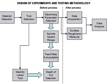
Figure 14. Design of experiments and testing methodology. Divided in two phases, the before process and the after process. ... 24

Figure 15. Photo of the grooving process used for experimentation. ... 29

Figure 16. Measurement method description. ... 30

Figure 17. Statistical analysis methodology used to reach the best model to predict surface roughness... 33

Figure 18. Example of a regression calculus results. ... 36

Figure 19. Resultant acceleration model response for 7075-T6 aluminum and ap = 1.5 mm. ... 37

Figure 22. Feed per tooth influence on the measured surface roughness. ... 39

Figure 23. Measured vs Predicted Ra for 7075-T6 aluminum at an ap of 1.5 mm and 0.08 mm/t of feed per tooth. ... 40

(11)

Figure 28. Measured vs Predicted Ra for 7075-T6 aluminum at an ap of 3.5 mm

and 0.18 mm/t of feed per tooth. ... 42

Figure 29. Resultant Acceleration prediction model response for 6061-T6 aluminum at an ap of 1.5 mm. ... 43

Figure 32. Feed per tooth influence on the measured surface roughness. ... 45

Figure 39. Resultant Acceleration prediction model response for 1045 Steel. ... 49

Figure 40. Axial depth influence in the measured surface roughness. ... 50

Figure 41. Measured vs Predicted Ra for 1045 Steel at an ap of 0.2 mm and 0.065 mm/t of feed per tooth. ... 51

Figure 42. Measured vs Predicted Ra for 1045 steel at an ap of 0.8 mm and 0.065 mm/t of feed per tooth. ... 51

Figure 43. Measured vs ideal surface roughness comparison in 7075-T6 aluminum for fz = 0.08 mm/t. ... 53

Figure 47. Measured vs ideal surface roughness comparison in 1045 steel for fz = 0.065 mm/t. ... 55

Figure 48. Acceleration of the three axis without cutting. ... 56

Figure 49. Comparison between theorical and real surface roughness... 61

Figure 50. Charge amplifier front panel of a Kistler 5211. ... 93

Figure 51. Terminal data types of LabView. Graphic obtained from National Instruments documentation [LabView Help]. ... 96

Figure 52. CScope subVi connection scheme... 96

Figure 53. DAQBasic subVi connection scheme. ... 98

Figure 54. DBK17 subVi connection scheme. ... 99

Figure 55. CP5512 MPI photo. ... 101

Figure 56. 30.6215 tool datasheet [Karnasch tool catalog]. ... 104

Figure 57. 30.6215 tool datasheet [Karnasch tool catalog]. ... 105

(12)

(13)

Figure 84. Matrix Plot with the correlation of all factors for 1045 Steel. The

(14)

LIST OF TABLES

LIST OF TABLES

Table 1. Parameters and variables that influence the surface quality of machined

parts in an end milling process. ... 5

Table 2. Relevant articles reviewed in the literature research phase. ... 8

Table 3. Instrumentation levels classification. ... 10

Table 4. Composition of the materials used in the experimentation. ... 25

Table 5. Tool characteristics and recommended process parameters. ... 26

Table 6. Ranges in the parameters used for machining in aluminum... 27

Table 7. Ranges in the parameters used for machining in 1045 Steel. ... 28

Table 8. Feed Rate values used for aluminum and the 30.6215 tool ... 28

Table 9. Feed Rate values used for steel and the 30.6472 tool. ... 29

Table 10. Example of a table made from all data acquired from one block. ... 31

Table 11. Final table of averages. ... 32

Table 12. Models obtained with multiple regression analysis, and their corresponding parameters. ... 59

Table 13. Instrumentation comparison between the ITESM and the IAI in Spain.. 62

Table 14. Amplifiers configuration. ... 93

Table 15. Data of populations observed to obtain the Q-Q Plot. ... 111

Table 16. Correlation matrix between factor for 7075-T6 aluminum... 114

Table 17. Data used for regression analysis for 7075-T6 aluminum. ... 116

Table 18. Regression summary output for the resultant acceleration prediction in 7075-T6 aluminum. ... 117

Table 19. Second regression summary output for the resultant acceleration prediction in 7075-T6 aluminum. ... 118

Table 20. Regression summary output for the surface roughness prediction and fz = 0.08 mm/t in 7075-T6 aluminum... 121

Table 22. Data of populations observed to obtain the Q-Q Plot for 6061-T6 aluminum... 127

Table 23. Correlation matrix between factor for 6061-T6 aluminum... 129

Table 24. Data used for regression analysis for 6061-T6 aluminum. ... 130

Table 25. Regression summary output for the resultant acceleration prediction in 6061-T6 aluminum. ... 131

Table 28. Data of populations observed to obtain the Q-Q Plot in 1045 Steel. ... 140

Table 29. Correlation matrix between factor for 1045 Steel. ... 142

Table 30. Data used for regression analysis for 1045 Steel. ... 143

Table 31. Regression summary output for resultant acceleration prediction in 1045 Steel. ... 144

(15)

LIST OF SYMBOLS

AccRes Resultant acceleration ap Axial Depth of Cut (mm)

ax Vibration in the x axis (mm/s2)

ay Vibration in the y axis (mm/s2)

az Vibration in the z axis

Β Coefficients for multiple regression analysis

D Tool diameter (mm)

fn Feed per revolution

fz Feed per tooth (mm/tooth) g Acceleration basic unit

r Toroidal end mill radius/turning insert radius Ra Average surface roughness (µm)

Rmax Maximum surface roughness (µm)

Rth Theorical surface roughness (µm)

S Spindle Speed (rpm)

Vc Cutting Speed (m/min)

Vf Feed Rate (mm/min)

(16)

Chapter 1: Introduction

Chapter 1: Introduction

The present study is made with the objective of continuing with an extended research in the topic of surface quality and the machining parameters involved in it. In order to narrow the topic of the present these, it will be focused in the surface quality of parts machined in a High Speed end-Milling (HSM) process. To achieve such objectives, a software based data acquisition platform is developed to measure variables through different sensing methods, allowing future research. A methodology, next explained, is followed to end with a resulting model which will help to predict a value for surface roughness in an end milling process. Similarly it will be understand the impact of each parameter analyzed in the final output quality characteristics.

1.1 Antecedents

Several attempts have been made to model the surface roughness of parts in machining processes. Dislike a turning process, an end-milling process has greater complexity. Models obtained by researchers have included a great number of parameters concluding that all of them have an effect on the final surface texture of the part. It is important to mention that almost none of these research works include vibrations as an independent factor related with the quality of parts and most of them have worked with low spindle speeds which are not a characteristic of an HSM process. Even though vibrations has an specific influence depending on several factors such as machine rigidity, tool wear, setup parameters, etc. a first attempt to include vibrations into an equation to predict surface roughness will be made.

1.2 Objectives

(17)

surface quality of the parts machined, in a high speed end milling process. Four main objectives are sought in this study:

1. Establish a technological platform capable of monitoring a high speed machining at high frequency sampling.

2. Determine the effect that the controllable parameters, spindle speed, depth of cut, feed per tooth and feed rate, have on the final Surface roughness (Ra) in aluminum and steel alloys machining.

3. Analyze and predict the machine vibrations (Acc[x]) based in machining parameters.

4. Create efficient surface roughness predictors for 3 different materials using statistical analysis tools.

5. Compare theorical versus measured Ra.

1.3 Methodology

(18)

Chapter 1: Introduction Literature Revision Software Platform Development Testing Protocol Lobule Stability Testing Selection of Parameter values Testing Data Analysis Model Selection Conclusions Journals Thesis Books LabView 7.1 IAI Chatter Detection System Data Acquisition System Testing Data Dependencies and correlations

RESULTS STEPS TOOLS

Kondia Machining Center Monitoring System Accelerometers Sensors SPSS Software Microsoft Excel Literature Revision Software Platform Development Testing Protocol Lobule Stability Testing Selection of Parameter values Testing Data Analysis Model Selection Conclusions Journals Thesis Books LabView 7.1 IAI Chatter Detection System Data Acquisition System Testing Data Dependencies and correlations

RESULTS STEPS TOOLS

Kondia Machining Center Monitoring System Accelerometers Sensors

[image:18.612.149.467.51.348.2]

SPSS Software Microsoft Excel

(19)

Chapter 2: High Speed Machining

2.1 Introduction to High Speed Machining

The High Speed Machining (HSM) technology was born in the last decades focused on increasing productivity in manufacturing industries. Due to the high spindle and feed rate velocities, less time is required to manufacture parts, and so, less production costs. Because it’s a relatively new technology, lots of studies have been and are being made around the topic, most of them centralized in the surface quality of parts. Drivers and motor technological advances have made possible to achieve speeds up to 30000 rpms and high feed rates, mostly in the aeronautic and aerospace industries. But the increment of such parameters has highlighted a tremendous problem in machining centers: their capability to control and monitor the process.

(20)

Chapter 2: High Speed Machining

Tool Variables Setup Variables Workpiece Variables

Tool Geometry Tool Nose Radius Tool Diameter Number of teeth Tool Wear Tool Vibration Tool Material

Machine-Tool Rigidity

Spindle Speed Feed Rate Depth of Cut Approach Angle

Stepover

Workpiece Material Workpiece Hardness Workpiece Geometry

Table 1. Parameters and variables that influence the surface quality of machined parts in an end milling process.

2.2 Why High Speed Milling?

It is very important for the metalworking industry to reduce costs in manufacturing, for such reason the development of high speed machines has been inspired. It is important also to recognize that high speed machining technology is relatively new, thus there is not enough knowledge on the most suitable shop procedures for these processes. These and other reasons are found to justify the research on such topic.

HSM implies high spindle speed, feed rates, or both. It could not be standardized a certain speed to be consider a high speed milling process, due to the condition and complexity of the process and the materials used, but it is known that HSM helps to improve productivity compared to a conventional milling method. The problem surges in which parameter settings to choose to achieve great quality parts if such process nature is not well know.

The development of material technology is driving the research on faster machining methods. New harder and resistant materials, mostly from automotive and aeronautic industries, cannot be machined with conventional processes.

(21)

- With the ability of increasing speed over six times, HSM will reduce production times and consequently production costs.

- Generating low cutting forces with HSM than with conventional milling, it is now possible to produce thinner-walled parts than normal.

- A single HSM has the potential to replace 2 or 3 conventional mills.

The development of such machinery is driving other areas involved in this industry to develop new technologies to satisfy the users of HSM. These evolutions involve:

- Complex and more resistant tools.

- Higher speed spindles.

- More complex control systems.

- Development on sensorial systems.

- Development on safety systems.

- New and more precise CNC systems.

- More rigid and resistant machine structures.

- Complex clamping methods.

- Research and development of new coolant methods.

For all these reasons and the need of knowledge in this area, this these focus its research in High Speed Milling.

2.3 Literature Review

(22)

Chapter 2: High Speed Machining

Figure 2. Surface Roughness parameter Ra representation over a specific length [Lou, Mike. et al, 1998].

Researchers have modeled the machining process in order to obtain an equation which help to predict the superficial roughness in parts [Boothroyd and Knight, 1989].

r f

Ra n

32 2

= (Equation 1)

Equation 1 shows the ideal surface roughness in turning, where Ra is the average value of surface roughness through a distance, fn is the feed per

revolution and r the tool radius. In addition to the geometric parameters in equation 1, researches have found that the surface roughness is affected by a great number of parameters and aspects in more or less magnitude. Models, such as the one of Lou, had include parameters like spindle speed, feed rate and depth of cut to determine Ra [Lou et al, 1999]. In other investigation Mandara left the depth of cut constant and varied the tool size getting the same results as Lou, which are, all parameter evaluated have an effect on surface roughness [Mandara et al, 1999].

(23)

Article name Authors Article Objective Observations Conclusions Optimization of

feedrate in a face milling operation using a surface roughness model (October 1999)

Dae Kyun Baek Tae Jo Ko Hee Sool Kim (South Korea)

Create a surface roughness

prediction based on geometric calculus of the axial and radial insert runouts. Process: face milling

Velocities used: Feed Rate 127 mm/min

Spindle Speed 370 rpm

Maximum Velocities: Vc = 116 m/min

A surface roughness predictor was created with prediction errors of 3 µm average. Measured surface roughness are about 13 and 20 µm.

Simulation of surface roughness and profile in high-speed end milling (2001)

Ki Yong Lee Myeong Chang Kang

Yung Ho Jeong Deuk Woo Lee Jeong Suk Kim (South Korea)

Present a method for simulating the machined surface using the

acceleration signal instead of using cutting forces. A geometric end milling model was used for modeling the end milling offset and tilt angle.

Process: Profiling

Velocities used: Feed per tooth: 0.05 mm/t Spindle Speed 10000-15000 Max Velocities: Vc = 471 m/min

The frequency analysis is used to obtain the dominant frequencies which are included in the model to obtain the surface roughness predictions. Errors vary in maximum 0.50 µm.

Surface roughness model for en milling: a semi-free cutting carbon casehardening steel (EN32) in dry condition (October 2000) A. Mansour H. Abdalla F. Meche (Egypt, UK) Develop a mathematical model that utilizing the response surface roughness methodology and method of experiments to predict the surface roughness. Process: face milling

The milling process was in dry conditions. Models and design of experiments too complex. Max Velocities: Vc = 38 m/min

Confidence intervals for Ra prediction were created.

Experimental study of surface

roughness in slot end milling AL2014-T6 (May 2003) Ming-Yung Wang Hung-Yen Chang (Taiwan) Analyze the influence of cutting condition and tool geometry on surface roughness when slot end milling AL2014-T6.

Process: slot end milling

Parameters considered were cutting speed, feed, depth of cut, concavity and axial relief angles of the end cutting edge of the end mill. Max Velocities: Vc = 80 m/min

Using response surface models two theoretical models were created for dry machining and with coolant. An adaptive-network based fuzzy inference system for prediction of workpiece surface roughness in end milling

(October 2001)

Ship-Peng Lo Predict the workpiece surface roughness after the end milling process with an adaptive network based fuzzy inference system. Process: N/A Three milling parameters were analyzed, spindle speed, feed rate and depth of cut. Max Velocities: Vc = 89 m/min

The predicted surface roughness values derived from ANFIS achieved very satisfactory accuracy.

This these Process: Grooving Vc = 830 m/min

(24)

Chapter 2: High Speed Machining 2.4 Proposed Modeling Approach

Several techniques can be used to obtain a final model for surface roughness. In this study regression methods will be used because of their simplicity, effectiveness and the allowance of using high exponential orders. As explained in the introduction of this work vibration and surface roughness will be our final predicted dependant values. Our dependant variables will be feed rate, spindle speed and depth of cut. Further study could be considered using different techniques to obtain the model in order to compare efficiency and processing time. Average surface roughness (Ra) will be kept as the unique term analyzed to get uniformity in the results of the experimentation phase. Next figure shows the proposed modeling approach for this study.

Ra

Vibration

_{Feed per Tooth}

Feed Rate &

Spindle Speed

Depth of Cut

Ra

Vibration

_{Feed per Tooth}

Feed Rate &

Spindle Speed

Depth of Cut

Figure 3. Proposed modeling approach scheme.

(25)

Chapter 3: Machining Monitoring System

3.1 Introduction

The present chapter is intended to give an overview of how a machine monitoring system (MMS) is composed. For better understanding, the whole MMS is divided into instrumentation levels. These levels can be seen in Table 3, where it is shown which type of instrumentation belongs to each level. Starting from the end milling machine, up to the computer, where the results are displayed and analyze, every possible instrument that was intended to use in the system is briefly explained. It is not the purpose of this these to deeply explained their operating mechanism but at least to know which function they have in the whole system. In order to acquire deeper information on the instrumentation, the bibliography shown at the end of this study should be consulted.

Level Instrumentation

Level 1 All type of sensors: accelerometers, acoustic emission, proximity, proper machine system, etc.

Level 2 Signal conditioners: amplifiers, filters, etc.

Level 3 Signal digitalizing/acquisition: Data Acquisition Cards, specific data acquisition devices, etc.

Level 4 Computer and software for signal displaying and processing.

Table 3. Instrumentation levels classification.

3.2 Instrumentation

(26)

Chapter 3: Machining Monitoring System instrumentation systems used by researchers will be shown. Next, each integrant of the system will briefly be explained. Technical information, data sheets and manufacturers can be found on appendix A.

Accelerometers Acoustic Emission DaqBoard Data Acquisition Card Compuscope Data Acquisition Card CNC Machine Controller MPI CARD Process Parameters A M P L I F I E R S Accelerometers Acoustic Emission DaqBoard Data Acquisition Card Compuscope Data Acquisition Card CNC Machine Controller MPI CARD Process Parameters A M P L I F I E R S In te rn al Se ns ors Accelerometers Acoustic Emission DaqBoard Data Acquisition Card Compuscope Data Acquisition Card CNC Machine Controller MPI CARD Process Parameters A M P L I F I E R S Accelerometers Acoustic Emission DaqBoard Data Acquisition Card Compuscope Data Acquisition Card CNC Machine Controller MPI CARD Process Parameters A M P L I F I E R S In te rn al Se ns ors

Figure 4. Instrumentation setup for data acquisition.

3.3 Sensors

(27)

3.3.1 Accelerometers

Accelerometers are piezoelectric sensors which are commonly used to measure vibrations and accelerations in most monitoring systems with industrial applications such as predictive maintenance, aerospace, automotive, medical, process control, etc. These sensors come in many types depending on the operation principle. Generally most accelerometers have a crystal which generates a signal when it is compressed by a force or ‘g’ force. The signal delivered by these sensors is commonly treated as m/s2. Further integration of data could give us measures as velocities or distances [Transductores y medidores electrónicos, 1977]. Data could be worked either in time or frequency domain. This signal could then be amplified and measure by an acquisition system which will then process it to convert it to the units of interest. Most accelerometers are housed in order to be used under harsh environment circumstances.

(28)

Chapter 3: Machining Monitoring System

Figure 5. Typical axial accelerometer [Endevco Homepage]

3.3.2 Acoustic Emission Sensors

Acoustic emission sensors have the same principle as the accelerometers; the only difference is that they do not use a seismic mass. Instead they use a ceramic disk or cylinder with a thickness of a few mm. Acoustic emission sensors are not widely known in engineering. They can be used as vibration sensors with very low amplitude and of very high frequency (in orders of 10 KHz to over 1 MHz). Depending on the type of sensor and its application, the sensitivity of an AE sensor can be given in V/um when the sensor is used to measure surface displacement motion, or in V/(mm/s) when the sensor is intended to measure surface velocity.

AE sensors are now starting to be used in numerous processes with monitoring purposes such as:

- Metal cutting

- Metal forming such as stamping and deep drawing

- Extruding plastic melts, specially filled melts

- Indicating the stress level in bolts

- Monitoring of welding processes

- Machinery condition monitoring and incipient failure detection

- Monitoring of aircraft structures.

(29)

accelerometers instead AE sensors due to their frequency range development, their simplicity to reduce noise, calibration methods and available bibliographic information.

AE sensors have the greatest sensitivity to the critical process conditions in precision machining, with the lowest noise level. Other sensors such as force and vibration sensors suffer from inaccuracies due to their low sensitivity in the extremely high frequency range, where most of the micro cutting activities are sensed [Dornfeld, 2003]. If the signal of interest is vibrations purely related to the cutting process, not to mechanical effects, AE sensors must be a good option.

Figure 6. Sensor types and location in the machining center.

Two acoustic emission sensors are used to sense vibrations in the high speed milling process for this study. Further analysis is made in order to determine the differences found on the experiment results, due to the used of different type of sensors (AE and Accelerometers).

(30)

3.3.3 Microphones

In the effort of searching different ways of measuring vibration on machining process, microphones were tested. As conventional microphones, industrial microphones emit signals due to vibrations caused by sound waves. These sound waves are emitted directly from the machining process. Their sensibility is directly related with the area of the sensor diaphragm. This factor is very important at the time of selecting the correct microphone [Transductores y medidores electrónicos, 1977]. Normally, the signal emitted by these sensors is measured in dB. The principal disadvantages detected on microphones are their low sensitivity and their reaction to environmental noise. It resulted very difficult to suppress noise signal caused by environmental noises of machining floors. Because their closed placement to the tool and workpiece, and their difficulty in the signal processing, these sensors were excluded from the machine instrumentation for the experimentation of the present study.

Figure 8. Microphone function principle [How stuff works homepage].

3.3.4 Multicomponent Force Sensors

(31)

compression force is positive. Multicomponent force sensors are devices with several built in common force sensors or dynamometers. These sensors are placed in order to detect two, three or more axes of measurement. These are mainly built with quartz and for high temperature or high sensitive applications. 3-component force sensors have a pair of quartz elements cut for longitudinal piezoelectric effect for measuring the compression force (the z component Fz) and a pair of quartz elements cut for the shear effect each for measuring the shear components (the x component Fx and the y component Fy) of the acting force [Gautschi, G, 2003]. The output of these devices is normally connected to a charge amplifier. The sensors could be connected in parallel so the output of the multicomponent sensor would be the sum of forces, or they could be measured separately.

Due to the need of a high number of amplifiers and the cost of the equipment, forces will not be measured in this work. The possibility of measuring forces in a high speed milling process will lead to interesting findings and should be included later in a machining model. Actually these sensors are being used to develop control systems, controlling parameters such as spindle speed and feed rate for specific purposes, like tool wear and surface roughness.

(32)

Chapter 3: Machining Monitoring System 3.4 Data Acquisition Cards

After signal amplifiers, Data Acquisition Cards (DACs) constitute the third level of instrumentation. DACs are electronics cards dedicated to signal acquiring and processing. Equally as sensors, several characteristics must be taken into account in order to select and appropriate DAC for a monitoring system. These characteristics include:

- Sampling Rate

- Input Tension

- Number of Analog Channels

- Number of Digital Channels

- Internal RAM Memory

Sampling rate prevails as the most important factor involved in selecting a DAC. This parameter is defined as the velocity at which the acquisition card will obtain data, this is, the maximum number of samples per second that will be obtained from the system. It is important to know that the number of data per sampling can also be configured. As computers with RAM Memory, this important factor heavily influences the cost of the DAC. A good sampling rate is considered to be around 100 kHz, depending on the measuring needs.

Input tension is the maximum voltage the DAC will deliver or admit from external components. Expressed in volts, normally DACs input voltage can be, +/- 5V, +/-10V or +/-12V. The input tension is directly related with the sensor for signal acquisition and with the type of channel, digital or analog, which are explained later.

(33)

Some advanced DACs are available with internal memory. The advantage of these cards is that they acquire and can process part of the signal obtained. This will avoid the computer processor to become slower during the signal acquisition. Their main disadvantage is the high cost.

For data obtaining and processing, three DACs are used in the experimentation related to this study. Daq2000 and Daq2005 from Iotech are responsible of the accelerometers signal and a CompuScope 1602 from Gage Applied will acquire the signal from the AE sensors.

Figure 10. Gage CompuScope 1602 acquisition card. Their analog inputs were used to acquire information from AE sensors at 2.4 Mhz maximum [Gage-applied Homepage].

3.5 Amplifiers

Amplifiers are used in electronic systems to increment devices output signals making possible for computers to be detected and analyzed. Most of sensorial instrumentation detects and emits signals in order of millivolts. These signals must be amplified so variations in detection can be clearly identified. Amplifiers can be divided into two categories: operational amplifiers and charge amplifiers.

(34)

Chapter 3: Machining Monitoring System units, such as velocity or acceleration units requires further software conversion, incrementing processing time. Depending on the amplifying factor its how sensitive the detection to sensor variations will be. Amplification factor must be adjusted taking into consideration the voltage ranges of the acquisition cards. Using amplifications which outputs voltages higher that DACs capacities may result into hardware damage.

Charge amplifiers have the same purpose than operational amplifiers, but their output its proportional to the charge received by the sensor [Chicala, 2004]. The voltage delivered by these type of amplifiers is proportional, in a scale, to the signal detected by the sensors. For such reason sensitivity and scale information must be configured to the amplifier. This information must be obtained from the sensor properties.

The accelerometers used for our study use a charge amplifier for each sensor. The amplifier used is a Kistler 5011 as shown in Figure 11. The configuration and connection scheme can be consulted in Appendix B.

Figure 11. 5011 Kistler Charge Amplifier use with each accelerometer. [Kistler Homepage]

3.6 Data Acquisition Software

(35)

DaqView, LabView, etc. All of them have weak and strong points which are described next.

- Mathlab.- Excellent software for control of processes and communication with acquisition cards. Easy programming makes this software an excellent choice. One of its weak points is that is not suitable for displaying information graphically.

- DaqView.- Software provided with acquisition cards. It is used mostly as a test software due to its simplicity and cost. It does not provide great programming capabilities, for such reason its application is limited.

- LabView.- For much the best visualization and easy programming software. It provides a complete library of preprogrammed functions which can be easily used. Its programming is completely graphical, but it can be programmed by some languages such as C, C++, etc. Its step by step function is a powerful tool which helps correcting and understanding complex programs.

LabView version 7.1 is the tool used to create the software which helped to obtain data and save it into disk so it can be analyzed. It also shows real time information graphically. This software, produced by National Instruments, counts with pre-realized VIs (named given to the graphical blocks) which makes the communication simple with the Daqs (2000 and 2005) and the Compuscope 1602. This is a very important aspect to consider before choosing the right software, and even more important, the acquisitions cards that are going to be used. Appendix C shows both VIs mentioned and their input and output signals.

Figure 12 shows a snapshot of the software developed, which has the next capabilities:

- Simultaneous and coordinated acquisition of data from three different acquisition cards, the Daqboard 2000, the Daqboard 2005 and the Compuscope 1602.

(36)

- An HMI which shows, in real time, the acquisition of different data.

- Ability to change acquisition configurations in its HMI.

- Simultaneous to data from acquisition cards, it acquires and shows information from the process. This is done through the MPI installed in the milling machine. For more information on the MPI consult appendix D.

- Finally it has the capability of saving all information showed in a .txt file in order to be analyzed after the process is finished.

Figure 12. MAP, acquisition platform developed to gather sensorial information of the machining process and vibrations.

3.7 State of the Art

(37)

the programming languages mostly used. Accelerometer and acoustic emission sensors are also widely used.

While more sensors are used in the monitoring system more difficult becomes the process and its location. Some researchers such as Lou and Chen uses proximity sensors to capture process parameter information like spindle speed. Using open architecture controls such as the 840D of Siemens provides the possibility of avoiding this kind of sensors that sometimes obstruct machine movements.

Compared to this monitoring system there are some differences in the way of acquiring information. Most researchers found in literature use a system as the one showed in Figure 13.

Figure 13. Lou and Chen experimental setup [Lou and Chen, 1999].

(38)

Chapter 3: Machining Monitoring System 3.8 Conclusions

The monitoring system developed has several advantages over typical systems used by researchers. Some of these advantages are:

- Avoids using sensors to gather machining parameter information, such as spindle speed, depth of cut and feed rate.

- Capture simultaneously information from several acquisition cards.

- All information is gathered once, this means data obtained at a certain time corresponds to the instant of acquisition of all other cards.

- Cards and channel can be shut down if they are not going to be used. This reduces processing time.

(39)

Chapter 4: Design of Experiments

A phase of high importance in the present work is the design of experiments and testing. In this chapter all conditions selected for experimentation will be supported. In the next section, the methodology followed during the whole research will be graphically shown.

4.2 Methodology Material Selection Tool Selection Machining Parameter Selection Data Acquisition Spindle Speed Range Feed Rate Computation Depth of Cut Selection Stability Lobes Test Surface Roughness Measure Data Analysis After process Before process

DESIGN OF EXPERIMENTS AND TESTING METHODOLOGY

Material Selection Tool Selection Machining Parameter Selection Data Acquisition Spindle Speed Range Feed Rate Computation Depth of Cut Selection Stability Lobes Test Surface Roughness Measure Data Analysis After process Before process

[image:39.612.106.519.307.630.2]

DESIGN OF EXPERIMENTS AND TESTING METHODOLOGY

(40)

Chapter 3: Design of Experiments 4.3 Material Selection

In the beginning of this these was commented that the present work is focused on High Speed Machining Processes. Some of the industries in which high speed processes are applied are aeronautics and automotive. For such reason the selection of materials was based on this assumption.

All the materials used are actually employed in parts produced by these industries. They were carefully selected in order to permit a comparison and a representative conclusion of the present work. Three materials were used in the experimentation phase, 7075-T6 Aluminum, 6061-T6 Aluminum and 1045 Steel. The following table shows some important characteristics of these materials that lead to its selection.

7075-T6 Aluminum 6061-T6 Aluminum 1045 Steel

Composition Si: 0.40

Fe: 0.50 Cu: 1.2-2.0 Mn: 0.30 Mg: 2.1-2.9 Zn: 5.1-6.1 Ti: Zr0.20 Cr: 0.18-0.28

Si: 0.721 Fe Cu: 0.408 Mn: 0.109 Mg: 0.937 Zn: 0.176 Ti: 0.051 Pb: 0.002 Cr: 0.072

C: 0.43-0.50 Mn: 0.60-0.90 P max: 0.040 S max: 0.050 Si max: 0.20-0.35

Brinell Hardness 145 88 220

Table 4. Composition of the materials used in the experimentation.

It was intended to use different materials which covered a wide range of hardness, in this case, Brinell Hardness from 88 to 220 will show its effect in surface quality and sensorial acquisition. Appendix E shows details of the material properties.

4.4 Tool Selection

(41)

machining parameters such as machining tool, range of spindle velocities, depth of cut, feed rates, etc. Even though it looked impossible, most of these parameters depended directly from the tool selected for each material, then, careful tool selection helped to remain in equal condition as possible all the experiments. A unique tool manufacturer was selected for all materials to avoid differences in the results due to the final tool treating.

The relation of the material with its tool is as follow:

- 7075-T6 Aluminum Tool Model: 30.6215 - 6061-T6 Aluminum Tool Model: 30.6215 - 1045 Steel Tool Model: 30.6472

Table 5 shows the model of each Karnasch tool used for the three materials tested, as its characteristics according to the manufacturer catalog.

Tool Model Tool Specifications Recommended Process Parameters 30.6215 Diameter = 12 mm

Radius = 1.5 mm Tooth number = 2

Cutting Velocities m/min = 300-1000 Feed per tooth mm = 0.08 – 0.18 RPM Range = 8000 - 26000 30.6472 Diameter = 10 mm

Radius = 1.5 mm Tooth number = 2

Cutting Velocities m/min = 300 – 400 Feed per tooth mm = 0.065

RPM Range = 12000 - 16000

Table 5. Tool characteristics and recommended process parameters. Note: The RPM range was obtained according to equation 2.

π

dx Vcx

S = 1000 (Equation 2)

where:

(42)

Chapter 3: Design of Experiments As the table shows, the diameter of the tool had to be changed for its use in steel, in order to maintain the radius of the tool constant. The radius of the tool is known to have a greater effect in the surface roughness than the diameter, this way the changes on surface quality from one material to another will not be greatly affected by the tool characteristics. More information from the tools used may be found in appendix F.

4.5 Machining Parameter Selection

A key issue to ensure representative results in the experimentation phase is machining parameter selection. Ranges from every parameter must be selected to avoid getting out of the limits permitted by the tool, the machine and the material. The stability lobes were an important tool that helped to choose the correct machining parameters, avoiding the influence of the machine static vibrations in the result. The stability lobes are explained in the next section.

Three machining parameters had to be defined for the experimentation phase: spindle speed (S), feed rate (Vf) and depth of cut (ap). Each of these parameter is greatly influenced by the tool used and the material machined. In the case of the spindle speed, it was consulted the tool catalog in order to cover all the range of possible velocities. As expected, the tool used for aluminum (30.6215) covers a wider range of speeds, than the one used in steel (30.6472). Table 6 and Table 7 show the ranges used for each parameter mentioned, in both materials.

Material:7075-T6 and 6061-T6 Aluminum Range

Spindle Speed 8000 – 22000 rpm

Feed Rate Calculated with: Vf = fz x S x Z

Depth of Cut 1.5, 2.5 and 3.5 mm

Note: fz (feed per tooth) was obtained from the catalog, using both limits of 0.08 mm/tooth and 0.18 mm/tooth. Z (number of teeth) of the tool is 2.

(43)

Material:1045 Steel Range

Spindle Speed 11000 – 16000 rpm

Feed Rate Calculated with: Vf = fz x S x Z

Depth of Cut 0.2, 0.4, 0.6 and 0.8 mm

Note: fz (feed per tooth) was obtained from the catalog, using 0.065 mm/tooth. Z (number of teeth) of the tool is 2.

Table 7. Ranges in the parameters used for machining in 1045 Steel.

For aluminum the increments of the spindle speed in each sample is 1000 rpm, for steel each sample was machined with an increment of 500 rpm. Grooves in the material were made to get each sample of the experimentation. Parameters remained constant in each groove. Table 8 and Table 9 shows the feed rates used for all cases.

For fz = 0.08 mm/tooth (Aluminum) For fz = 0.18 mm/tooth (Aluminum)

RPM Vf (mm/min) RPM Vf (mm/min)

8000 1280 8000 2880

9000 1440 9000 3240

10000 1600 10000 3600

11000 1760 11000 3960

12000 1920 12000 4320

13000 2080 13000 4680

14000 2240 14000 5040

15000 2400 15000 5400

16000 2560 16000 5760

17000 2720 17000 6120

18000 2880 18000 6480

19000 3040 19000 6840

20000 3200 20000 7200

21000 3360 21000 7560

22000 3520 22000 7920

Table 8. Feed Rate values used for aluminum and the 30.6215 tool

For fz = 0.065 mm/tooth (Steel)

RPM Vf (mm/min)

(44)

Chapter 3: Design of Experiments

13000 1690 14000 1820 15000 1950 16000 2080

Table 9. Feed Rate values used for steel and the 30.6472 tool.

The stability lobe test was used for the depth of cut selection. Generally this method helps avoiding entering chatter zones during machining by selecting a depth of cut that produces stable machining conditions. Appendix G explains more detailed the effect of this test in the machining parameter selection.

4.6 Surface Roughness Measure

After the machining of parts follows the measuring of surface roughness. The specific machining process selected for experimentation is grooving. As Figure 15 shows, several 100 x 180 x 25 mm blocks were used for testing. In these blocks grooves were made keeping constant the machining parameters in each one. Each groove corresponds to a specific spindle speed, depth of cut and feed rate.

Figure 15. Photo of the grooving process used for experimentation.

(45)

eliminate vibrations due to a thin wall. The numeric control program for machining was made parametric to make changes simple, it can be seen in Appendix H.

After machining a stylus profilometer was used to measure the surface roughness in the plane of the groove. Because of the anatomy of the profilometer, measurements had to be done 40 mm after the groove ends, in the sense of machining. Figure 16 shows the way the measurement was taken. A 5 mm surface was measured, obtaining the average of all data taken (Ra)

(46)

Chapter 3: Data Analysis

Chapter 5: Data Analysis

This chapter shows the overall approach used for data analysis. Detailed tables and procedures are included in appendix I.

5.2 Experimental Results

The software application developed provided the capability of saving all data acquired for further analysis. The processing of the information was time consuming due to the size of the files. Two files are saved: a) the information of acoustic emission sensors and information from the MPI and b) the data from the accelerometers. Two files are obtained from each block machined. Then each file has information from a specific depth of cut and all the grooves made on the block. After acquiring both files they are joined in one table using a spreadsheet. The software is made considering that it has to save the same number of data in both files. Once all data joined in a table an average value of all parameters in each groove was obtained. Table 10 shows an example of a fragment of the table constructed with all data obtained.

Index AE 1 AE 2 S Vf ap ax ay az … …

22 206.04 26.55 8000 2880 1.5 214.018 194.362 26.4078 … … 23 209.34 22.57 7999 2880 1.5 269.490 240.929 26.5423 … … 24 205.18 23.40 7999 2880 1.5 302.068 277.816 26.6098 … …

… … … … … … … … … … …

Table 10. Example of a table made from all data acquired from one block.

(47)

used to graph the results and compare vibrations with the surface roughness obtained.

S ax ay az _Ra

8000 335.40 288.14 267.45 1.36

9000 430.12 330.35 262.16 1.61

10000 505.17 400.82 263.34 2.02

11000 436.41 377.22 260.00 1.90

12000 617.45 422.56 266.32 2.00

13000 568.87 405.77 256.90 2.17

14000 478.10 367.65 249.75 1.54

15000 421.96 409.78 270.28 1.80

16000 543.67 435.34 253.99 1.91

17000 458.52 362.03 253.18 1.61

18000 385.15 355.45 245.69 1.57

19000 363.78 340.83 254.69 2.32

20000 364.62 324.54 270.60 2.34

21000 444.24 379.19 277.13 2.39

22000 342.35 367.29 272.51 2.36

Table 11. Final table of averages.

As it may be seen in the previous table is obtained only one final value of vibration of each sensor and of Ra, corresponding to a spindle speed, which was maintained constant through the length of the groove.

5.3 Model Type Selection

(48)

Chapter 3: Data Analysis

Hypothesis Analysis Q-Q Plots

Correlation Analysis Normal Distribution?

Yes No

Multiple Regression

STATISTICAL ANALYSIS METHODOLOGY

Hypothesis Analysis Q-Q Plots

Correlation Analysis Normal Distribution?

Yes No

Multiple Regression

STATISTICAL ANALYSIS METHODOLOGY

Figure 17. Statistical analysis methodology used to reach the best model to predict surface roughness.

(49)

of the model have a linear correlation with surface roughness, if not it is important to consider that the factor must be of a higher order to be influent or important in the prediction.

Finally, several multiple regression models are obtained an evaluated with its prediction capability and only the important parameters are the ones that remain in the model, making it more simple.

(50)

Chapter 6: Surface Roughness Models

Chapter 6: Surface Roughness Models

Final results are presented in this chapter. Surface roughness prediction models with their corresponding coefficients are shown. As explained in the last chapter two models are obtained for each material. The first parameters and their interactions will form a model which predicts the resultant 3 axis vibrations. Then, a second model will include the force parameters and the predicted vibration to predict the final surface roughness. For more information about the application of the regression analysis to the data, and the results of such analysis (ANOVA tables) appendix I should be consulted.

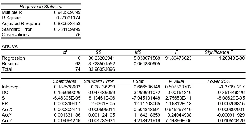
6.2 Regression Data Analysis

There are several factors resulting from the regression data analysis that are important at the time of deciding which model is more precise. The most important factor is the R Square parameter. This parameter offers a percentage of efficiency at which the model is capable of correctly predicting the surface roughness. The coefficients of the ANOVA table, which indicate the value that must be assigned to the β values of the model. It could have a negative sign, which means that has an inverse influence. In the same table there is a column assigned as P-Value, which is a statistical parameter that indicates the significance of the factors in the whole model. This parameter determines which parameter should be deleted from the model, due to its low contribution in the prediction.

(51)

SUMMARY OUTPUT Regression Statistics Multiple R 0.943509799 R Square 0.89021074 Adjusted R Square 0.880523453 Standard Error 0.234159999 Observations 75 ANOVA

df SS MS F Significance F Regression 6 30.23202941 5.038671568 91.89473623 1.20343E-30 Residual 68 3.728501552 0.054830905

Total 74 33.96053096

[image:51.612.106.504.69.271.2]

Coefficients Standard Error t Stat P-value Lower 95% Intercept 0.187538603 0.28136299 0.666536148 0.507323702 -0.37391217 DC -0.156689326 0.047486059 -3.299691072 0.00154316 -0.251446226 S -6.46305E-05 8.13461E-06 -7.945131448 2.75653E-11 -8.08629E-05 FR 0.000319417 2.6361E-05 12.11703065 1.19812E-18 0.000266815 AccX 0.000302411 0.000599014 0.504848591 0.615297416 -0.000892901 AccY 0.001331186 0.001124105 1.184218659 0.24044938 -0.000911929 AccZ 0.019964249 0.004732634 4.218421916 7.44866E-05 0.010520429

Figure 18. Example of a regression calculus results.

6.3 Model Results

(52)

Chapter 6: Surface Roughness Models 6.4 7075-T6 Aluminum Model

90 experiments were conducted in 7075-T6 aluminum. After several multiple regression analysis the next final model to predict the resultant acceleration was obtained. The resultant acceleration signal used in all materials is given as the square root of the sum of squares of the signals of the X, Y and Z accelerometer. Due to the nature of the process, the most relevant signals were obtained from the Y and Z axis. The X axis signal was less significant, because the grooving was made perpendicular to this axis.

) * 10 86818 . 5 ( ) * 05 89473 . 2 ( ) * 448764 . 0 ( 44 . 1556

Re 2 3

S E S E S s

Acc =− + + − − + −

The model is able to predict the resultant acceleration of machined parts with a 50% of effectiveness (Adjusted R-Square in the ANOVA table). It is evident that the spindle speed plays an important role in this prediction.

Figure 19, Figure 20 and Figure 21 show how the predicted resultant acceleration follows the real one at each depth of cut.

AccRes Prediction 0 200 400 600 800 1000

8000 10000 12000 14000 16000 18000 20000 22000

Spindle Speed (rpm)

A

ccR

es (m

g

)

fz = 0.08 mm fz = 0.18 mm Predicted AccRes

ap = 1.5 mm Al 7075-T6

(53)

AccRes Prediction

0 200 400 600 800 1000

8000 10000 12000 14000 16000 18000 20000 22000

Ac

cRe

s (

m

g

)

ap = 2.5 mm Al 7075-T6

Figure 20. Resultant acceleration model response for 7075-T6 aluminum and ap = 2.5 mm.

AccRes Prediction

0 200 400 600 800 1000

8000 10000 12000 14000 16000 18000 20000 22000

Ac

cR

e

s (

m

g

)

ap = 3.5 mm Al 7075-T6

Figure 21. Resultant acceleration model response for 7075-T6 aluminum and ap = 3.5 mm.

(54)

Chapter 6: Surface Roughness Models 7075-T6 Aluminum 0.000 0.500 1.000 1.500 2.000 2.500

8000 10000 12000 14000 16000 18000 20000 22000

Spindle Speed (rev/min)

S u rf ace Ro u g h n ess ( u m)

fz=0.08 & ap=1.5 mm fz=0.08 & ap=2.5 mm fz=0.08 & ap=3.5 mm fz=0.18 & ap=1.5 mm fz=0.18 & ap=2.5 mm fz=0.18 & ap=3.5 mm fz: feed per tooth (mm) ap: axial depth of cut (mm)

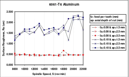
Figure 22. Feed per tooth influence on the measured surface roughness.

The model for fz = 0.08 resulted with very low precision, then it will not be

shown in this chapter, and the model for fz = 0.18 mm/t has the following form.

) Re * * 07 00655 . 8 ( ) Re * 00525252 . 0 ( ) * 0005969 . 0 ( 03638 . 2 s Acc Vf E s Acc Vf Ra − − + + − =

Both summary outputs are shown in appendix I. For the first model we have

an efficiency of 6%. With this data we assume that the model is not capable of

making any good surface roughness prediction. In Figure 22 we can see that the

values of Ra with fz of 0.08 mm/t does not change considerably with different

values of spindle speed. This may be one of the reasons why the efficiency of the

model resulted very low.

In the other case the model for fz = 0.18 mm/t resulted with an efficiency in

prediction of 38%, much higher than the first model. Even though it is a very low

value, the next figures show both models prediction capabilities comparing the

(55)

Measured vs Predicted Ra 0 0.2 0.4 0.6 0.8

8000 10000 12000 14000 16000 18000 20000 22000

S u rf ace R o u g h n ess (u m ) 0% 20% 40% 60% 80%

Measured Ra Predicted Ra % Error

ap = 1.5 mm fz = 0.08 mm/t

Al 7075-T6

Figure 23. Measured vs Predicted Ra for 7075-T6 aluminum at an ap of 1.5 mm and 0.08 mm/t of

feed per tooth.

Measured vs Predicted Ra

0 0.2 0.4 0.6 0.8

8000 10000 12000 14000 16000 18000 20000 22000

S u rf ac e R oughne ss (u m ) 0% 20% 40% 60% 80% 100%

ap = 2.5 mm fz = 0.08 mm/t

Al 7075-T6

(56)

Chapter 6: Surface Roughness Models

0 0.2 0.4 0.6 0.8

8000 10000 12000 14000 16000 18000 20000 22000

S u rf ac e R oughne ss (u m ) 0% 20% 40% 60% 80% 100%

ap = 3.5 mm fz = 0.08 mm/t

Al 7075-T6

Figure 25. Measured vs Predicted Ra for 7075-T6 aluminum at an ap of 3.5 mm and 0.08 mm/t of feed per tooth.

0 0.5 1 1.5 2 2.5

8000 10000 12000 14000 16000 18000 20000 22000

S u rf ace R ough n ess ( u m ) 0% 20% 40% 60% 80% 100%

ap = 1.5 mm fz = 0.18 mm/t

Al 7075-T6

(57)

Measured vs Predicted Ra 0 0.5 1 1.5 2 2.5

8000 10000 12000 14000 16000 18000 20000 22000

S u rf ace R o u g h n ess (u m ) 0% 50% 100% 150% 200%

ap = 2.5 mm fz = 0.18 mm/t

Al 7075-T6

Figure 27. Measured vs Predicted Ra for 7075-T6 aluminum at an ap of 2.5 mm and 0.18 mm/t of feed per tooth.

0 0.5 1 1.5 2 2.5

8000 10000 12000 14000 16000 18000 20000 22000

S u rf ac e R o u g h n ess (um ) 0% 20% 40% 60% 80% 100%

ap = 3.5 mm fz = 0.18 mm/t

Al 7075-T6

(58)

Chapter 6: Surface Roughness Models 6.5 6061-T6 Aluminum Model

A total of 90 tests were conducted in 6061-T6 aluminum (15 levels of spindle speed, 3 levels of depth of cut and 2 levels of feed per tooth). This aluminum is softer than the 7075-T6. After several multiple regression analysis the next final model was obtained to predict the resultant acceleration.

) * 10 7859 . 7 ( ) * 05 7889 . 3 ( ) * 582462 . 0 ( ) * ( * 13 1152 . 2 79161 . 2186 Re 3 2 3 S E S E S S ap E s Acc − + − − + − − − =

The model resulted able to predict 69% of the real acceleration. In this model it is more notorious the influence of the spindle speed jointly with the depth of cut. An example of how this model works is shown in Figure 30.

8000 10000 12000 14000 16000 18000 20000 22000

A ccR es ( m g )

ap = 1.5 mm Al 6061-T6

(59)

8000 10000 12000 14000 16000 18000 20000 22000

A ccR es ( m g )

ap = 2.5 mm Al 6061-T6

Figure 30. Resultant Acceleration prediction model response for 6061-T6 aluminum at an ap of 2.5 mm. AccRes Prediction 0 200 400 600 800 1000

8000 10000 12000 14000 16000 18000 20000 22000

A ccR es ( m g )

ap = 3.5 mm Al 6061-T6

Figure 31. Resultant Acceleration prediction model response for 6061-T6 aluminum at an ap of 3.5 mm.

Two other models were obtained for this aluminum also. As in the 7075-T6

aluminum, the model for fz = 0.08 mm/t resulted very ineffective. Next equation

corresponds to the model of fz = 0.18 mm/t.

) Re * * 07 85312 . 6 ( ) Re * 003675913 . 0 ( ) * 00049374 . 0 ( 982117576 . 0 s Acc Vf E s Acc Vf Ra − − + + − =

The model for fz = 0.08 mm/t works with an efficiency of 3 %, very low

(60)

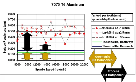
Chapter 6: Surface Roughness Models aluminum the differences between the Ra of both fz are huge. This can be seen in Figure 32. 6061-T6 Aluminum 0.000 0.500 1.000 1.500 2.000 2.500

8000 10000 12000 14000 16000 18000 20000 22000

Spindle Speed, S (rev/min)

S u rf ace R o ughne ss , R a ( u m )

fz=0.08 & ap=1.5 mm fz=0.08 & ap=2.5 mm fz=0.08 & ap=3.5 mm fz=0.18 & ap=1.5 mm fz=0.18 & ap=2.5 mm fz=0.18 & ap=3.5 mm fz: feed per tooth (mm) ap: axial depth of cut (mm)

Figure 32. Feed per tooth influence on the measured surface roughness.

An example of how each model works comparing the real versus the predicted Ra is shown next.

0 0.1 0.2 0.3 0.4 0.5 0.6

8000 10000 12000 14000 16000 18000 20000 22000

S u rf ac e R ough ne ss (u m ) 0% 20% 40% 60% 80% 100%