Interval and Fuzzy Regressions to Enhance DRASTIC Aquifer Vulnerability Assessments-Edición Única

INSTITUTO TECNOLÓGICO Y DE ESTUDIOS SUPERIORES DE MONTERREY

PRESENTE.-Por medio de la presente hago constar que soy autor y titular de la obra denominada"

, en los sucesivo LA OBRA, en virtud de lo cual autorizo a el Instituto Tecnológico y de Estudios Superiores de Monterrey (EL INSTITUTO) para que efectúe la divulgación, publicación, comunicación pública, distribución, distribución pública y reproducción, así como la digitalización de la misma, con fines académicos o propios al objeto de EL INSTITUTO, dentro del círculo de la comunidad del Tecnológico de Monterrey.

El Instituto se compromete a respetar en todo momento mi autoría y a otorgarme el crédito correspondiente en todas las actividades mencionadas anteriormente de la obra.

De la misma manera, manifiesto que el contenido académico, literario, la edición y en general cualquier parte de LA OBRA son de mi entera responsabilidad, por lo que deslindo a EL INSTITUTO por cualquier violación a los derechos de autor y/o propiedad intelectual y/o cualquier responsabilidad relacionada con la OBRA que cometa el suscrito frente a terceros.

Interval and Fuzzy Regressions to Enhance DRASTIC Aquifer

Vulnerability Assessments-Edición Única

Title Interval and Fuzzy Regressions to Enhance DRASTIC Aquifer Vulnerability Assessments-Edición Única

Authors Lizeth Guadalupe Oliva Soto

Affiliation ITESM-Campus Monterrey

Issue Date 2008-05-01

Item type Tesis

Rights Open Access

Downloaded 19-Jan-2017 05:35:24

CAMPUS MONTERREY

DIVISIÓN DE INGENIERÍA Y ARQUITECTURA PROGRAMA DE GRADUADOS EN INGENIERÍA

Interval and fuzzy regressions to enhance DRASTIC aquifer vulnerability assessments

TESIS

PRESENTADA COMO REQUISITO PARCIAL PARA OBTENER EL GRADO ACADÉMICO DE:

MAESTRO EN CIENCIAS

ESPECIALIDAD EN SISTEMAS AMBIENTALES

POR:

LIZETH GUADALUPE OLIVA SOTO

CAMPUS MONTERREY

DIVISIÓN DE INGENIERÍA Y ARQUITECTURA PROGRAMA DE GRADUADOS EN INGENIERÍA

Los miembros del comité de tesis recomendamos que la presente tesis de la Ing. Lizeth Guadalupe Oliva Soto sea aceptada como requisito parcial para obtener el grado académico de Maestro en Ciencias especialidad en:

SISTEMAS AMBIENTALES

Comité de Tesis:

___________________________ _________________________________ Dr. Venkatesh Uddameri Dr. Jürgen Mahlknecht

Co-asesor Co-asesor

_________________________________ Dr. Kim D. Jones

Sinodal

Aprobado:

______________________________ Dr. Joaquín Acevedo Mascarúa

Director de Investigación y Posgrado de la Escuela de Ingeniería

iii RESUMEN

Interval and Fuzzy Regressions to Enhance DRASTIC Aquifer Vulnerability

Assessments

(Mayo 2008)

Lizeth Guadalupe Oliva Soto, Ingeniera Química, ITESM-Monterrey.

Co-asesores: Dr. Jürgen Mahlknecht y Dr. Venkatesh Uddameri

La técnica de toma de decisiones llamada DRASTIC es ampliamente utilizada en los

Estados Unidos y en otros lugares para evaluar la vulnerabilidad de acuíferos a la

contaminación. Esta técnica incluye una cantidad considerable de incertidumbre en el

proceso. El uso de regresiones con intervalos y “fuzzy” ha sido propuesta en este estudio

para obtener los pesos relativos de los criterios en DRASTIC. La vulnerabilidad del

acuífero se relacionó con la concentración de contaminante observada usando una

función exponencial de riesgo-utilidad. Seis diferentes regresiones de intervalo y “fuzzy”

fueron evaluadas en la rápidamente creciente región de México central delimitada por el

subsistema del acuífero de Silao-Romita. Los resultados de este estudio indicaron que la

técnica convencionalmente usada en DRASTIC generalmente subestima la vulnerabilidad

en áreas urbanas y en ciertas áreas agrícolas, mientras que las regresiones con intervalos

y “fuzzy” reflejaron resultados más acordes a la situación real del área. Índices de

semejanza fueron desarrollados para evaluar las capacidades de predicción de los

modelos. Los modelos de regresión “fuzzy” que fueron desarrollados utilizando la técnica

iv

Pedrycz mejoró la capacidad de predicción de la regresión con intervalos y de la técnica

clásica de Tanaka. En general, fue notado que el uso de los modelos de regresiones

“fuzzy” en conjunto con la función exponencial de utilidad resultó más útil para captar la

incertidumbre que surge de las diferencias entre las personas que realizan la toma de

v

ACKNOWLEDGMENTS

This journey has brought me a lot of learning: professional, personal, even within some

sports! I could not have achieved this degree if it was not because of the resources from

different people and institutions. I am grateful to all of them:

• My family, which were always there to help me. Thank you all for believing in

me!

• Part of this research was funded by the Consejo de Ciencia y Tecnología de

Guanajuato (CONCyTEG) under the treaty 04-12-A-044 of the Fondo Mixto

Guanajuato and the Cátedra Uso Sustentable del Agua from the ITESM-Campus

Monterrey.

• Scholarships were provided by the College of Engineering (Dr. W. Heenan and

Mr. T. Hinojosa) of Texas A&M University-Kingsville and the Departamento de

Becas de Posgrado from the ITESM-Campus Monterrey.

• All of the committee members (Dr. Venkatesh Uddameri, Dr. Jürgen Mahlknecht

and Dr. Kim D. Jones) because of trusting in my capabilities, teaching me far

beyond school knowledge, letting me grow and gain experience by working with

them, and always guiding and helping me out.

• A third scholarship was provided by my friend Annette Hernandez (Definitely not

everybody lets you stay in their home for months!).

vi

• Ing. Ignacio Luján, Ing. Xavier Pérez and all of their laboratory staff at the

ITESM-Campus Monterrey, because of letting me analyze some samples in their

laboratories.

• My group mates both in Monterrey and in Texas, for sharing their experience and

knowledge with me.

• Last but not least, I am grateful to all the friends who were with me all along the

way: I do not want to list names… I am surely going to miss a lot of people who

vii

TABLE OF CONTENTS

ABSTRACT... iii

ACKNOWLEDGMENTS ...v

TABLE OF CONTENTS... vii

LIST OF FIGURES ...ix

LIST OF TABLES ...xi

1.0 INTRODUCTION ...1

2.0 RESEARCH GOALS AND OBJECTIVES ...6

3.0 BACKGROUND ...8

3.1. DRASTIC vulnerability index methodology...8

3.2. Introduction to interval and fuzzy numbers...9

3.2.1. Interval numbers...9

3.2.2. Fuzzy numbers ...9

3.3. Interval and fuzzy regressions ...12

3.3.1. Interval regression approach ...12

3.3.2. Fuzzy regression based approaches...13

3.3.3. Savic and Pedrycz approach ...18

3.3.4. Similarity index concept ...19

3.3.5. Construction of the defuzzified maps...21

4.0 STUDY AREA DESCRIPTION AND DATA GATHERING...22

4.1. Study area description ...22

4.2. Data compilation and pre-processing ...26

4.2.1. Sampling for the Silao-Romita aquifer subsystem...27

5.0 DEVELOPMENT OF THE DRASTIC MAPS...31

6.0 RESULTS AND DISCUSSION...35

6.1. Final DRASTIC Maps...35

viii

6.2.1. Ordinary least squares regression results...37

6.2.2. Interval and fuzzy regression results ...38

6.3. Defuzzified maps ...48

7.0 SUMMARY AND CONCLUSSIONS ...56

8.0 REFERENCES ...58

APPENDIX A. RATINGS AND WEIGHTS FOR THE CONVENTIONAL DRASTIC .. APPROACH...63

APPENDIX B. ADAPTED RATINGS FOR SELECTED DRASTIC PARAMETERS .66 APPENDIX C. OBSERVED NITRATE CONCENTRATIONS ...67

APPENDIX D. INPUT DATA FOR REGRESSION ANALYSYS FOR DEPTH,... RECHARGE, IMPACT AND HYDRAULIC CONDUCTIVITY. ...68

APPENDIX E. BASE MAPS FOR AQUIFER MEDIA, SOIL MEDIA, AND ... TOPOGRAPHY ...72

APPENDIX F. PARAMETER VALUES OBTAINED FROM THE INTERPOLATED... MAPS INCLUDED IN INTERVAL AND FUZZY REGRESSIONS ...74

APPENDIX G. RECLASSIFIED DRASTIC MAPS FOR EACH PARAMETER...75

APPENDIX H. VBA SUBROUTINES FOR THE CALCULATION OF SIMILARITY .. INDICES ...79

ix

LIST OF FIGURES

Figure 1. A triangular symmetric membership function [adapted from Hojati et al.

(2005)]. ...11

Figure 2. Membership functions and a α-cut [adapted from Tanaka (1996)]...12

Figure 3. A fuzzy linear relationship [from Hojati et al. (2005)]...14

Figure 4. A certain observed interval [from Hojati et. al (2005)]. ...15

Figure 5. Illustration of deviational variables ...17

Figure 6. Illustration of deviational variables (2)...18

Figure 7. Similarity between two fuzzy numbers [from Hojati et al. (2005)]. ...20

Figure 8. Similarity between observed and predicted interval numbers ...20

Figure 9. Location of Silao-Romita aquifer (Instituto Nacional de Estadística, Geografía e Informática, 2005a; Comisión Estatal de Aguas de Guanajuato, 2005)...22

Figure 10. Extraction permits and major cities in Silao-Romita aquifer (Comisión Estatal de Aguas de Guanajuato, 2005) ...24

Figure 11. Land Use-Land Cover and Nitrate concentrations for Silao-Romita aquifer (Comisión Estatal de Aguas de Guanajuato, 2005)...24

Figure 12. Estimated vulnerability vs. Nitrate concentrations...29

Figure 13. Sampled sites within Silao-Romita aquifer. Aquifer boundary from Comisión Estatal de Aguas de Guanajuato (2005)...29

Figure 14. Flow chart for the integration of the DRASTIC parameters map. ...32

Figure 15. Depth IDW-interpolation for Silao-Romita aquifer ...33

Figure 16. Depth Thiessen Polygons map for Silao-Romita aquifer ...33

Figure 17. Depth composite map for Silao-Romita aquifer...34

Figure 18. Nitrate interpolated map...36

Figure 19. DRASTIC indices vulnerability map...37

Figure 20. Nitrate concentrations vs. Depth from Land Surface and well-depth ...41

Figure 21. Maximum, minimum and average for the similarity index for different methods. ...44

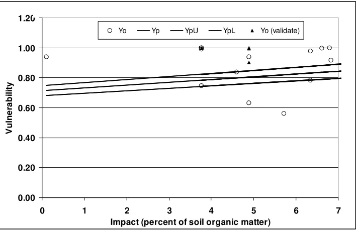
Figure 22. Interval regression (S&P) observed and predicted nitrate concentrations. ...45

Figure 23. Interval regression observed and predicted nitrate concentrations...45

Figure 24. Classical Tanaka (S&P) observed and predicted nitrate concentrations ...46

Figure 25. Classical Tanaka observed and predicted nitrate concentrations ...46

Figure 26. Observed and predicted nitrate concentrations using HSB1 (S&P). ...47

Figure 27. Observed and predicted nitrate concentrations using HSB1...47

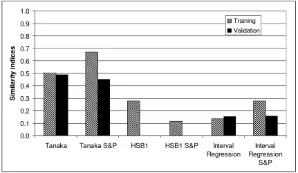
Figure 28. Similarity indices for training and validation sets. ...48

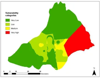
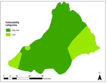
Figure 29. Defuzzified map based on interval regression (S&P), classical Tanaka (S&P) and HSB1(S&P) weights for DRASTIC. ...49

Figure 30. Defuzzified map based on interval regression weights for DRASTIC...50

Figure 31. Defuzzified map based on classical Tanaka weights for DRASTIC...50

Figure 32. Defuzzified map based on HSB1 weights for DRASTIC...51

x

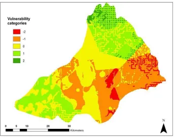
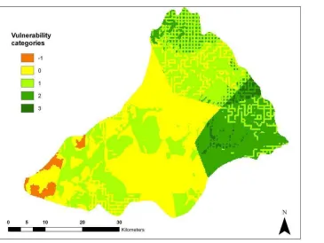
Figure 34. Comparison of categories of vulnerability between DRASTIC conventional

approach and the interval regresión...52

Figure 35. Comparison of categories of vulnerability between DRASTIC conventional approach and the classical Tanaka approach ...53

Figure 36. Comparison of categories of vulnerability between DRASTIC conventional approach and the HSB1 regression...53

Figure 37. Aquifer media map (Comisión Estatal de Aguas de Guanajuato (2005)...72

Figure 38. Soil texture map (Instituto Nacional de Estadística, Geografía e Informática, 2005a) ...73

Figure 39. Elevation map (Instituto Nacional de Estadística, Geografía e Informática, 2005a) ...73

Figure 40. Depth reclassified map...75

Figure 41. Recharge reclassified map...75

Figure 42. Aquifer media reclassified map...76

Figure 43. Soil media reclassified map...76

Figure 44. Topography reclassified map ...77

Figure 45. Impact of the vadose zone (percent of soil organic matter) map ...77

xi

LIST OF TABLES

Table 1. Parameters in DRASTIC vulnerability index [from Aller et al. (1987)]. ...8

Table 2. Description of the data collected ...27

Table 3. Root Mean Square Error for the IDW interpolated maps for depth, recharge and impact ...34

Table 4. Ordinary least squares regression for Silao-Romita Aquifer ...38

Table 5. Mid-points and Half-widths for regular interval and fuzzy regressions ...39

Table 6. Mid-points and Half-widths for interval and fuzzy regressions when combined with S&P approach...39

Table 7. Regression coefficients and confidence intervals for well-depth and depth to groundwater table against nitrate concentrations ...41

Table 8. Classical Tanaka and HSB1 coefficients without conductivity outliers ...42

Table 9. Average influence of each parameter in vulnerability predictions ...43

Table 10. Vulnerability categories tags and intervals...49

Table 11. Matrix of the inter-comparison between the vulnerability categories of the DRASTIC conventional approach, interval and fuzzy regressions. Under-estimated percentages...54

Table 12. Matrix of the inter-comparison between the vulnerability categories of the DRASTIC conventional approach, interval and fuzzy regressions. Correctly-estimated percentages...54

Table 13. Matrix of the inter-comparison between the vulnerability categories of the DRASTIC conventional approach, interval and fuzzy regressions. Over-estimated percentages...55

Table 14. Ratings and weights for the conventional DRASTIC approach (Canter, 1997)63 Table 15. Aquifer media adapted ratings for permeability of the hydro-geologic units for Silao-Romita aquifer...66

Table 16. Soil texture adapted ratings for Silao-Romita aquifer...66

Table 17. Percent of Soil organic matter adapted ratings for Silao-Romita aquifer ...66

Table 18. Observed nitrate concentrations...67

Table 19. Location of sampled sites ...68

Table 20. Tabular data gathered for depth, recharge and impact ...69

Table 21. Results of Pumping tests for Silao-Romita aquifer (Ibarra, 2004) ...70

Table 22. Observations regarding the data used to build the DRASTIC maps...71

Table 23. Hydrogeologic units, based on permeability of the materials [taken from Comisión Estatal de Aguas de Guanajuato, 2005]. ...72

1

1.0INTRODUCTION

World population rose from two and half billion in 1950, to around six billion in 2000,

and continues to increase in many countries (UNESCO, 2006), causing an increase on the

demand for water resources. Currently, safe drinking water is not an available asset for

one fifth of the world population (Zaporozec, 2002). The increasing demand creates a

stress on this scarce resource. Therefore, research should focus on conserving water and

maintaining its quality.

In several regions of the world, groundwater accounts for a high proportion of the total

water supply. Groundwater is that defined as being below the water table in geologic

formations that are completely water saturated (Freeze and Cherry., 1994). The term

aquifer refers to any material that is able to store and transmit water (Stone, 1999), and

can provide water in sufficient quantity and quality for human consumption. Aquifers are

a very important source of water because: a) they have a very large storage capacity,

often greater than any built reservoir; b) they can be accessed drought periods; and c)

their water quality without pre-treatment, is usually better than untreated surface waters

(Morris et al., 2003), because due to natural filtration. In addition, the water is relatively

cheaper and easier to obtain compared to other drinking water sources, because it can be

extracted at the site where it will be consumed (Morris et al., 2003). Negative

consequences on the environment and human health can be expected if the quality of

these resources is lowered due to pollution. Industrial and urban activities, agriculture and

other point and non point sources can contribute to their pollution.

The vulnerability of an aquifer represents its sensitivity to be adversely affected by a

pollutant load (Foster and Hirata, 1991) and is determined by different factors. These

parameters include the hydraulic conductivity which is the resistance to water flow in the

strata within the vadose zone (above the water table), the chemical reactivity of the

____________

strata, the mobility and persistence of a pollutant as well as loading characteristics such

as the quantity, the concentration, and the manner and location (Zaporozec, 2002; Foster

and Hirata, 1991). The type of aquifer vulnerability that is only related to the

characteristics of the aquifer itself is called the “intrinsic vulnerability” (Antonakos and

Lambrakis, 2007; Zaporozec, 2002). Another type of vulnerability called specific

vulnerability, which includes both the intrinsic vulnerability and the characteristics of the

discharge of the pollutant (Antonakos and Lambrakis, 2007).

Apart from the type of pollutant involved, the scale at which aquifer vulnerability is

evaluated plays an important role in the characterization of groundwater vulnerability.

The scale may be regional, as in the Sole Source Aquifer Demonstration Program or local

like in the Protection of Wellheads Program. Both Sole Source Aquifer Demonstration

and Protection of Wellheads programs are carried out to comply with the Safe Drinking

Water Act amendments. The Sole Source Aquifer Demonstration Program focuses on

identifying “critical aquifer areas” (US Environmental Protection Agency, 2007). Thus,

regional scale mapping is utilized as a first step to delineate and recognize most

vulnerable areas within a region.

Currently, several methods exist to characterize aquifer vulnerability. These methods can

be divided into four categories (Focazio et al., 2002; Canter, 1997). The first category

includes the subjective rating or index methods. These are more policy and management

oriented, because results are given tags such as low, medium or high vulnerability

(Focazio et al., 2002). The statistical based methods are those that specify correlations

between contamination and aquifer properties (Canter, 1997). The process based methods

are those that simulate the fate and transport of contaminants to characterize vulnerability

(Comitte on techniques for assessing ground water vulnerability, 1993). Hybrid methods

are those that combine index based methods with statistical or process based methods

(Focazio et al., 2002).

In the index methods, the parameters are paired with ratings, which are site specific

index (Aller et al., 1987). A major limitation of index methods is that they usually do not

incorporate the pollutant characteristics (Focazio et al., 2002) and they only measure

intrinsic vulnerability. Some of the index based approaches are DRASTIC (Aller et al.,

1987), SINTACS (Civita and De Maio, 1997) and AVI (Ministry of Water, Land and Air

Protection, 2005). One critical short-coming of these methods is the subjectivity (Focazio

et al., 2002) imposed by the assignment of the weights by various decision makers

(Scanlon et al., 2003). To address the subject of specific vulnerability, some studies have

included observed pollutant concentrations, such as nitrates, for identification or

validation of vulnerability characterization (Antonakos and Lambrakis, 2007; Dixon,

2005b). Groundwater pollution due to nitrates is a major issue currently and agriculture is

considered one of the major sources of this compound (UNESCO, 2006). It is also “the

most pervasive contaminant in groundwater” (Scanlon et al., 2003) in the United States

and in Texas. Nitrates are usually salts that are highly soluble in water, under normal pH

conditions they do not easily sorb onto negatively charged particles (such as clay), ion

exchange is not a process in which they typically participate and do not usually volatilize

(Scanlon et al., 2003). Therefore, a great part of the surface generated nitrates percolate

through the vadose zone, and into the saturated zone. There are several sources of

nitrates. According to Canter (1997) they are classified as: natural, such as geologic

nitrogen and forests disturbances; waste materials, such as animal manures, sludge

applied to the ground, septic tanks wastes, and leachates from landfills; and those from

agriculture associated practices.

Some studies have combined index methods with statistical, information theoretic or

process based methods, such as descriptive statistics, logarithmic regressions and fuzzy

set theory, in order to decrease the subjectivity associated with index methods and to deal

with the uncertainty (Bailey et al., 2003) in the data. Antonakos and Lambrakis (2007)

combined the DRASTIC index methodology with descriptive statistics, logistic

regression and weight of evidence. These approaches were used to correlate the presence

of nitrates with the vulnerability of the study areas. Thirumalaivasan et al. (2003)

developed software where both ratings and weights of the DRASTIC parameters are

achieved using nitrate as nitrogen (NO3-N) concentrations. Fuzzy set theory (Zadeh,

1965), has also been combined with index methods in several studies. Dixon (2005a)

incorporated a fuzzy-rule based model into a geographic information system to derive a

DRASTIC vulnerability indices map. Some modifications to the conventional DRASTIC

approach were included, such as the generation of modified DRASTIC and Vulnerability

Index (VI) maps. Uricchio et al. (2004) characterized the vulnerability of an aquifer using

the SINTACS methodology, but also determined its risk as the product of this

vulnerability times a degree of hazard. The weights these authors gave for hazard were

based on fuzzy sets. Dixon (2005b) developed a neuro-fuzzy model for aquifer

vulnerability and carried out a sensitivity analysis of its application using GIS. The

parameters included in this vulnerability assessment were soil hydrologic group, depth of

the soil profile, soil structure and land-use. The validation of the results was carried out

by comparing vulnerability categories found using NO3-N concentrations against

categories predicted with the models. Chen and Fu (2003), and Zhou et al. (1999)

incorporated the fuzzy set theory into the DRASTIC methodology because many times

two sites reporting different values for certain parameters end up with the same rating.

The fuzzy set theory was combined with SINTACS vulnerability method to obtain

vulnerability indices (Di Martino et al., 2005).

Ordinary least squares regression (OLSR) is a statistically based approach that can be

applied to determine the weights for use with index method. For OLS, the estimators for

the coefficients of the regression are unbiased (Hamilton, 1991) under the assumption

that all errors have same mean and variance. Also, there are several conditions under

which the estimators of the coefficients and/or the statistics (such as F or t statistics) are

biased. Some of these conditions are that there is a non-linear relationship between

variables, an important factor is not included, and there are measurement errors

associated with the independent variables (Hamilton, 1991). Therefore, these situations

are limitations for the use of OLRS.

Fuzzy regressions are another method to calculate the weights. These regressions are

inputs to an output, which is treated as a fuzzy number. Fuzzy regressions do not require

complying with the assumptions mentioned for the OLSR (Uddameri and Honnungar,

2007). Therefore, the latter can be used more broadly. Fuzzy regressions are useful when

there is lack of sufficient data, no “assumptions about the statistical distribution” of the

real system can be made, the manner in which the variables are related is not clear,

“human judgment” is involved or when the output is fuzzy (Tran et al., 2002). In recent

times, fuzzy regressions have been used in many different environmental applications.

Tran et al. (2002) integrated a multi-objective fuzzy regression with the Revised

Universal Soil Loss Equation to determine how some factors affect soil erosion. Özelkan

and Duckstein (2001) incorporated the fuzzy regression and fuzzy least squares

regression into a conceptual rainfall-runoff model. Uddameri and Kuchanur (2004)

estimated the log K_oc-log K_ow relationship via a fuzzy regression. Uddameri and

Honnungar (2007) estimated groundwater budget parameters using fuzzy linear

regression. Fuzzy regression is an alternative approach that has not yet been used to

6

2.0RESEARCH GOALS AND OBJECTIVES

2.1.Overall goal

The main purpose of this study is to demonstrate the utility of the application of interval

and fuzzy regression approaches for characterizing aquifer vulnerability.

2.2.Specific objectives

The following objectives were identified and carried out in order to achieve the main

purpose of this study:

• The development of DRASTIC indices maps following the approach proposed by

Aller et al. (1987) to characterize the vulnerability of the Silao-Romita aquifer

subsystem in Guanajuato, Central Mexico.

• Application of interval regression (Chang and Ayyub, 2001) and different fuzzy

regressions (Hojati et al, 2005) as alternatives to determine the weights for the

DRASTIC methodology

o The fuzzy regression methods included are based on the minimization of

fuzziness criterion (classical Tanaka) (Chang and Ayyub, 2001; Hojati et al.,

2005) and Goal programming with inclusion of deviational variables (HSB1)

(Hojati et al., 2005)

o Assess whether the use of OLSR in combination with fuzzy regressions by using

Savic & Pedrycz approach (Chang and Ayyub, 2001) improves the performance

of the interval and fuzzy regressions to characterize aquifer vulnerability.

• Measure the performance of interval and fuzzy regressions predictions against field

observations.

• Develop aquifer vulnerability maps for the Silao-Romita aquifer using interval and fuzzy regressions and compare the resulting vulnerability categories against the

conventional DRASTIC vulnerability categories map.

• Intercompare the characterization of vulnerability maps derived from the application

The background for DRASTIC vulnerability indices methodology, fuzzy and interval

8

3.0BACKGROUND

3.1.DRASTIC vulnerability index methodology

The methodology chosen to characterize vulnerability in this study was the DRASTIC

index methodology. This methodology has been widely used for aquifer vulnerability

assessments in the US and other parts of the world (Hamza et al, 2006; Antonakos and

Lambrakis, 2007). The initials of the parameters used in this method comprise the word

DRASTIC. Each one of them is mentioned in Table 1(Aller et al., 1987):

Table 1. Parameters in DRASTIC vulnerability index [from Aller et al. (1987)]. Letter or initial Parameter

D Depth to groundwater

R Net recharge rate

A Aquifer media

S Soil media

T Topography (slope)

I Impact of the vadose zone

C Conductivity (hydraulic) of the aquifer

For vulnerability assessments this approach becomes a Multicriteria Decision Making

problem (Malczewski, 1999) as shown on Equation 1 (Aller et al., 1987). It is a weighted

linear combination of seven parameters.

W R W R W R W R W R W R W

RD R R A A S S T T I I C C

D + + + + + +

=

DVI (1)

Where the subscript R indicates the Rating obtained from field measurements, and the

subscript W indicates the Weight for each parameter that is assigned by the decision

maker. As mentioned previously, the assignment of the weights is a subjective process

and depends upon the risk preferences of the decision maker. As such, these weights are

3.2.Introduction to interval and fuzzy numbers

3.2.1. Interval numbers

An interval number is defined as “an ordered pair of real numbers,

[ ]

(Moore, 1966) as in Equation 2:

[ ]

{

}

An advantage of using interval numbers is that they can describe “approximate values

and an error bound, or an upper and a lower bound to the exact result” (Moore, 1966).

Interval numbers “will contain the entire set of possible values of the solution” for when

the input data or the coefficients vary within two values or to account for calculation

round-off errors (Moore, 1979). Therefore, interval numbers can be used to describe the

weights in the DRASTIC conventional approach because these weights vary within a

range due to the difference in opinions between the stakeholders regarding the relative

importance of each parameter. Fuzzy numbers explained next, can also be used to address

this issue.

3.2.2. Fuzzy numbers

The fuzzy set theory was first introduced by Zadeh (1965). A fuzzy set is defined as a

“class of objects with a continuum of grades of membership” (Zadeh, 1965). The

membership function, which can take any value from zero to one, defines how much the

parameter in the fuzzy set belongs to that set (Mukaidono, 2001). An illustration of these

functions is found in Figure 1, where it can be observed that the minimum value is zero

and the maximum value is one. An element belongs more to the set when the membership

function approaches one. Fuzzy numbers are special cases of fuzzy sets, which have the

characteristics of being normalized, i.e., at least one value in the set has a membership

value of one; and convex (Mavrotas et al, 2003), i.e.,“the membership value of any given

than the membership value of either end points”(Yen and Langari, 1998). Fuzzy numbers

“can be expressed as interval numbers with membership values” (Chang and Ayyub,

2001). These numbers are very useful “to deal with fuzzy data originated from a fuzzy

phenomenon” (Tanaka et al., 1989). The main purpose of fuzzy set theory is “to establish

a mathematical theory to deal with subjectivity” (Mukaidono, 2001) introduced either by

the model itself or by fuzzy data (Chang and Ayyub, 2001). An advantage of fuzzy

numbers over interval numbers is that fuzzy numbers provide more information on the

preference of a value. Therefore, fuzzy numbers are used to deal with the subjectivity

surrounding the weights of the DRASTIC vulnerability methodology.

Membership functions of fuzzy numbers can have different shapes (Dixon, 2005b),

trapezoidal, bell and triangular are some examples of them (Dixon, 2005). Triangular

symmetric membership functions are the most commonly used (Mavrotas et al., 2003)

and there are two elements that are used to describe them, a mid-point and a half-width

(Hojati et al., 2005). Being symmetric, the half-width extends from the mid-points

towards both sides. The graphical representation of these elements is shown in Figure 1,

Figure 1. A triangular symmetric membership function [adapted from Hojati et al. (2005)].

A triangular membership function can be decomposed into an infinite number of

triangular membership functions (Tanaka, 1996). An α cut creates a subset of elements

contained in one of these membership functions, which have membership values greater

or equal than a specific value. Thus, a total membership function can be built by

performing operations on several α cuts. An illustration of an α cut is shown in Figure 2,

resulting in a smaller set as denoted by the hatched area. The following section contains

the formulation of the regression approaches using both interval and fuzzy numbers . αj -cj αj αj + cj Aj

1.0

Figure 2. Membership functions and a α-cut [adapted from Tanaka (1996)].

3.3.Interval and fuzzy regressions

A regression model is developed to “describe how the dependent variable is related to the

independent variables” (Bardossy, 1990). This model gives a “prediction equation for the

entire population” based on “collected data with uncertainties” (Chang and Ayyub,

2001). The DRASTIC vulnerability index methodology is combined in this study along

with regression models to predict vulnerability and to gain insight from the model to

interpret what happens in reality. Based on the formulation is shown in Equation 1, the

independent variables are the ratings of the parameters and the DRASTIC vulnerability

index is the dependent variable.

3.3.1. Interval regression approach

This type of regression defines both the response variable and the coefficients of the

regression as interval numbers (Chang and Ayyub, 2001). The independent variables

remain crisp numbers. The approach followed is based on the one proposed by Chang

and Ayyub (2001). The interval regression applied in this study is of the form shown in

Equation 3.

ki k i

i

i A X A X A X

X A

The interval number that describes the predicted response variable is called Yˆ . The

independent variables data are denoted by Xij. The interval regression coefficients, Aj

~ ,

are defined by a mid point called m_jand a half-width c_j:

(

)

A~_j = _j, _j , ∀ =1,..., (4)

The objective function seeks to minimize the fuzziness of the model that is characterized

by the half-widths of the interval numbers. The number of parameters is denoted by k,

and the total amount of data points is n.

∑∑

, c j k

free

m_j = _j ≥ ∀ = (6)

The purpose of the following constraints is that the observed data should be contained

within all the predicted values for the response variable obtained with the model.

(

)

j

ij j

j , , 1,...

1 = ∀ ≤ −

∑

(

)

j

ij j

j , 1,...

1 = ∀ ≥ +

∑

3.3.2. Fuzzy regression based approaches

Fuzzy regressions are based on the concept of fuzzy numbers. There are two major

classes of fuzzy regressions, the ones that try to minimize the vagueness and those that

utilize the least squares of the errors (Chang and Ayyub, 2001). For both of these types of

(Hojati et al., 2005). An illustration of a fuzzy regression is shown in Figure 3, with a

centerline and lower and upper boundaries to the sides.

Figure 3. A fuzzy linear relationship [from Hojati et al. (2005)].

By using fuzzy regressions the predictions of the model can be obtained at different

levels of trust called “minimum degree[s] of acceptable certainty” (Hojati et al., 2005).

The minimum degree of certainty possible for a model is a specific membership degree of

the response variable (Hojati et al., 2005) called H. The subset that contains all the

elements in the response variable that have at least an H degree of membership value is a

“certain observed interval” (Hojati et al., 2005) and is shown in Figure 4. A lower level

of H indicates greater compatibility between the observed data and the fuzzy regression

Figure 4. A certain observed interval [from Hojati et. al (2005)].

3.3.2.1.Classical Tanaka approach and the vagueness approach criterion

The first fuzzy regression implemented is the one proposed by Tanaka (Hojati et al,

2005). This regression follows the form shown in Equation 9.

k j

x A x

A x A

Yˆ= _{1 1n} + _{2 2n} +...+ _{j jn}, ∀ =1,..., (9)

In Equation 9, Yˆ is the predicted response variable and is assumed to be a fuzzy number

with a symmetrical triangular shape. The termA_j is the coefficient of the fuzzy

regression. The coefficients are treated as fuzzy numbers with membership functions of a

symmetric triangular shape. A graphical representation of these fuzzy numbers is shown

in Figure 1. The center and half widths for the regression coefficient function are α_i and

j

c . For the fuzzy number y_ithat describes the observed response variable the mid-point

and half-width are denoted by y_i ande_i, respectively, and are known. The required

mid-point and half-width for the regression coefficients are obtained using the following

∑∑

This function minimizes the total “sum of the half widths of the predicted intervals”

(Hojati et al., 2005). The number of parameters is denoted by k, and the total number of

data points is n. The following constraints ensure the model generated certain intervals

encompass entire set of certain observed intervals.

(

)

(

)

(

)

∑

j H c x y H e i n

1 , ,..., 1 , 1 1

α (11)

(

)

(

)

(

)

∑

j H c x y H e i n

1 , ,..., 1 , 1 1

α (12)

. ,..., 1 ,

0

, c j k

free j

j = ≥ ∀ =

α (13)

As it is required that the certain predicted intervals contain the certain observed intervals,

the half-widths of the coefficient membership functions often tend to be large due to the

influence of outliers (Hojati et al., 2005).

3.3.2.2.Goal-programming HSB1 approach and the use of deviational variables

Another approach to fuzzy regression was proposed by Hojati, Bector and Smimou and is

called HSB1 in this thesis (Hojati et al., 2005). In this approach the independent variable

is crisp and the response variable and the coefficients of the regressions are treated as

fuzzy numbers. The membership functions for these fuzzy numbers are assumed to be

triangular and symmetric. Similarly, the mid-points and half-widths are named as

previously and denoted by α_i and c_j for the regression coefficient function, and y_i

ande_i for the observed response fuzzy number, respectively. The form of the fuzzy

regression is of the same manner as the previous approach, and is shown in Equation 9.

objective function (Equation 14), deviational variables are included in order to overcome

larger widths due to outliers (Hojati et al., 2005). Equations 15 and 16 describe the

constraints required to encompass the observed fuzzy number within the predicted fuzzy

number. However, unlike the classical Tanaka approach these constraints are treated as

soft goals through the use of deviational variables. In other words, it is desired that the

predicted intervals intersect or contain the observed intervals, but is not mandatory. Due

to this flexibility, the half-widths of the coefficients may be smaller than the ones found

using methods such as classical Tanaka which require a crisp intersection of H-certain

intervals.

(

)

∑

=

− + −

+ _{+ + +}

n

i

iL iL iU

iU d d d

d Minimize

1

(14)

Figure 5. Illustration of deviational variables

x

y

-x

y

d

d

-x

y

x

y

d

d

-Figure 6. Illustration of deviational variables (2)

Figures 5 and 6 depict the role of deviational variables in this formulation. As can be seen

from these figures, four variables are required to fully account for deviations between the

upper and lower observed and predicted values. Thus, the main purpose of this objective

function is to minimize these deviations (Hojati et al., 2005).

(

)

(

)

(

)

∑

j H c x d d y H e i n

1 , ,..., 1 , 1 1

α (15)

(

)

(

)

(

)

∑

j H c x d d y H e i n

1 , ,..., 1 , 1 1

α (16)

, ,..., 1 , 0 , ,

,d d d i n

d_iU+ _iU− _iL+ _iL− ≥ ∀ = (17)

. ,..., 0 ,

0

, c j k

free _j

j = ≥ ∀ =

α (19)

3.3.3. Savic and Pedrycz approach

Savic and Pedrycz (from now on referred to as Savic and Pedrycz or S&P) (Chang and

Ayyub, 2001; Hojati et al., 2005) integrated the results of an Ordinary Least Squares

formulate their objective functions. The coefficients of the OLSR are used as the

mid-points of the membership functions for the fuzzy coefficients. The minimization of the

fuzziness relies only on the half-widths of these membership functions. In this study it is

combined with both the interval and fuzzy regression approaches.

3.3.4. Similarity index concept

An assessment of how well models are able to match observed values is important. A

new evaluation measure called the similarity index was developed. For fuzzy numbers it

is the formulated as shown in Equation 19. It measures the proportion of overlapping

within the observed and predicted response fuzzy numbers as a fraction of the total areas

of the two fuzzy numbers.

P o OV P o OV P o A A A A A A A A index Similarity + = + − + −

=1 2 2 (19)

In the formula for the similarity index, A_Ois the area under the observed fuzzy response,

P

A is the area under the predicted fuzzy response and A_OV is the area where both fuzzy

numbers overlap. In Figure 7, yˆ is the predicted response fuzzy number and _i y_iis the

observed response fuzzy number. The similarity index is zero when the observed and

Figure 7. Similarity between two fuzzy numbers [from Hojati et al. (2005)].

An analogous approach was followed to calculate the similarity index for the interval

regression predictions vs. observed data. The similarity index was estimated as the degree

to which the observed interval number y_i and the predicted interval number yˆ _i

overlapped as shown in Figure 8. As with the fuzzy number case, the similarity index is

zero when the observed and predicted interval numbers do not overlap. In Equation 20,

which was used to calculate the similarity index for interval numbers, L_Ois the observed

fuzzy response, L_Pis the predicted fuzzy response and L_OV is the interval where both

numbers overlap.

Figure 8. Similarity between observed and predicted interval numbers

P o

OV

P o

OV P

o

L L

L L

L

L L L index

Similarity

+ = +

− + −

=1 2 2 (20)

Lp

y

ˆ

,

3.3.5. Construction of the defuzzified maps

Once the interval or fuzzy regressions equations have been established using a set of

input/output data it can be used to make predictions where only input data are available.

In particular, if the maps for DRASTIC ratings are available for a region, they can be

used in conjunction with the developed regression models to characterize regional aquifer

vulnerability. However, the predictions obtained from the interval and fuzzy regressions

have lower and upper limits and a most likely value. Therefore, the outputs (weights) of

the DRASTIC index, will also have these three values resulting in DRASTIC indices

composed of three maps: low, medium and high. The single final DRASTIC map can be

obtained via defuzzification. The centroid of the fuzzy number is used here for

defuzzification and given as (Kaufmann and Gupta, 1989):

4 *

2 _{M U}

L Y Y

Y function membership

fuzzy of

Centroid = + + (21)

In Equation 21, the term Y_L refers to the lower value, Y_M to the medium value, and Y_U to

the higher value at a given location. The methodologies discussed in this chapter were

applied to the Silao-Romita aquifer in México for illustrative purposes and are described

22

4.0STUDY AREA DESCRIPTION AND DATA GATHERING

4.1.Study area description

The aquifer subsystem of Silao-Romita is located in the state of Guanajuato, Central

Mexico (20.69º and 21.21º N and 101.07º and 101.76º W) with an area of 1979 km2. Its limits to the North and East are the Sierra de Guanajuato mountain range, and the

mountains in the Sierra de Pénjamo and El Veinte to the South and South West. The

study area is located in the zone 14 North Universal Transverse Mercator (UTM)

coordinate system (Instituto Nacional de Estadística, Geografía e Informática, 2005a).

The aquifer limits are shown in Figure 9. The neighboring aquifers include the cuenca

alta del río Laja, valle de Irapuato, Pénjamo-Abasolo, río Turbio, La Muralla and valle of

León. The most important cities in the area are Guanajuato, Silao, and Romita (Instituto

Nacional de Estadística, Geografía e Informática, 2005b).

A total of 1,984 extraction permits have been issued in the aquifer. The geographical

distribution of the wells is shown in Figure 10. Of these, 1697 are wells, 281 are

waterwheels and 6 are springs. Of the total number of permits, only 1,592 are active of

these, 1,390 are used for irrigation purposes, 176 for drinking water extraction, 15 for

industries and 11 for rangeland activities (Ibarra, 2004). As seen in Figure 10, the wells

tend to be clustered around the valleys, mainly within the cities and along the roads that

connect them with only a few wells located in the mountains.

The greatest precipitation occurs in the zones with higher elevations and can be 800 mm

annually. Lower altitude zones experience between 500 and 600 mm annually (Salas,

2004). The average annual precipitation over the entire study area was calculated to be

635 mm with a monthly potential evaporation of 158 mm (Ibarra, 2004).

Agriculture comprises the greatest amount of land area, as shown in Figure 11. The

forests are mainly located in the mountains of the Sierra de Guanajuato, which are the

mountains located in the North East section of the aquifer zone.

Several creeks are located in the Sierra de Guanajuato; however, the most important

waterways are the Silao and Guanajuato rivers, which flow in a southerly direction. The

north zone of the Sierra de Guanajuato tends to have sub-dendritic drainage and S and SE

radial drainage due to volcanic fingerprints. In the zone there are two springs that are

known their temperature, these are Comanjilla with 96°C, and Aguas Buenas with 46°C

(Salas, 2004).

The geomorphologic zones present in the area are the Sierra de Guanajuato, Bajío

Guanajuatense and the Sierra de Pénjamo (Mahlknecht and Oliva, 2005). The

physiographic provinces within this study area are the Mesa del Centro (Central Plateau),

with sub-provinces of Sierras and Llanuras del Norte de Guanajuato or Altos (Highlands)

of Guanajuato; and the province of Eje neovolcánico (Mexican Neo-volcanic belt), with

the subprovince of the Bajío (Lowlands) Guanajuatense (Salas, 2004; Consejo de

Figure 10. Extraction permits and major cities in Silao-Romita aquifer (Comisión Estatal de Aguas de Guanajuato, 2005)

The Bajío Guanajuatense is from tectonic origins in which medium consolidated material

(tertiary undifferentiated granular) and consolidated (alluvial) material deposits, and it is

characterized by valleys and hills (Mahlknecht and Oliva, 2005). Two areas are clearly

identified: the transition zone or pie-de-monte, which is where the runoff from the

mountains usually infiltrates and was formed out of erosion, and the cumulative plateau

at base level, which is where the wells and agricultural lands are typically located (Salas,

2004). The Mesa del Centro elevations are approximately 3000 meters above sea level,

with different levels of erosion (Salas, 2004). These mountains coincide with faults with

NW-SE orientation that are intersected by faults having a NE-SW orientation (Ibarra,

2004). There are two groups of rock formations, 1) those found in the valleys and hills

from the Tertiary period to now(Salas, 2004), and 2) those found in the Sierra de

Guanajuato from the Mesozoic period (Consejo de Recursos Minerales, 2004).

Localized intensive extraction has created a pronounced drawdown behavior in the

vicinities of the cities of Silao and Trejo. This moved the flow lines from the surrounding

mountains towards these depressed zones (Mahlknecht and Oliva, 2005). A great

proportion of the water that infiltrates near the mountains, do not reach the valleys, but

circulates in the fractured zones (Ibarra, 2004). This behavior around Silao has been

documented in other studies (Consejo de Recursos Minerales, 2004). It has also been

observed that west of Silao is a zone in which the water table levels have been rising, this

zone is recharged continuously and may be influenced by the Silao River. Another

recovery zone has been identified east of Silao, which may be influenced by the runoff

from the Sierra de Guanajuato. The characteristics of these mountains indicate that this

may cause storm-water peaks to be incorporated to groundwater through intermediate

flows (Cortés, 2001).

The existence of three different aquifers within several horizons in this study area has

been proposed by Cruz (1998). Meanwhile, other studies (Ibarra, 2004; Consejo de

Recursos Minerales, 2004) identify only two. The deeper aquifer is semi-confined (Cruz,

There may be transmisitions between shallower and deep water (Cruz, 1998; Ibarra,

2004), because their border is constituted of detached clay lenses (Consejo de Recursos

Minerales, 2004).

The Silao-Romita aquifer subsystem surroundings are classified as areas with medium

and scarce groundwater availability (AQUASTAT-FAO, 2000). One of the main

economic activities is agriculture that takes up to 80% of the water resources in the

watershed, of which groundwater accounts for almost 50% of the resources (Ibarra,

2004). The aquifer has been classified as overexploited by the Comisión Nacional del

Agua (Comisión Nacional del Agua, 2005), thus is prohibited from increasing extraction

permits and volumes. An increase in the total population is, however, expected; therefore,

the demand for water is also expected to increase (Comisión Nacional del Agua, 2004).

In recent years, there have been conflicts about the water resources between authorities in

the Silao-Romita watershed and in the adjacent areas (i.e. the city of León). This conflict

occurs because the latter one has already stressed its hydraulic resources to the limit and

its demand for water continues to rise (Escalante 2002).

4.2.Data compilation and pre-processing

The data necessary to generate the maps for the different parameters was obtained from

Table 2. Description of the data collected

Parameter Source Format

Depth to groundwater

2005 Sampling campaign Tabular

Net recharge rate Horst (2006) Tabular Aquifer media Comisión Estatal de Aguas de

Guanajuato (2005)

Vector (polygon) file.

Soil media Instituto Nacional de Estadística, Geografía e Informática (2005a)

Vector (polygon) file.

Topography (slope) Instituto Nacional de Estadística, Geografía e Informática (2005a)

Altitude level curves (vector file)

Impact of the vadose zone (% of soil organic matter)

2005 sampling campaign Tabular

Conductivity (hydraulic) of the aquifer

Ibarra (2004) Tabular

4.2.1. Sampling for the Silao-Romita aquifer subsystem

During October 2005, 30 samples were taken in and around the Silao-Romita aquifer, as

part of the project “Estudios isotópicos para el desarrollo de un modelo conceptual del

funcionamiento hidrodinamico del subsistema acuífero Silao-Romita, Estado de

Guanajuato” (Isotopic studies for the development of a conceptual model of the

hydrodynamic functioning of the Silao-Romita aquifer subsystem, Guanajuato State).

The funding for this project was provided by the Consejo de Ciencia y Tecnología de

Guanajuato (CONCyTEG) and the Catedra Andrés Marcelo Sada from the

ITESM-Campus Monterrey.

The distribution of these samples was not uniform due to the fact that many wells were

either no longer operating, temporarily out of service or not found within the vicinity of a

pre-determined sampling site. Those that were not in use but still functional, were started

and the sample was taken after at least 15 min of pumping. Of the 30 wells, four were

located outside of the study area. Filtration was achieved with a portable Nalgene® Filter

Holder with receiver, and using Millipore® 0.45 μm nitrocellulose filters for nitrate

samples and several other major ions and compounds. The analysis for nitrates was

Mexico using the method 300.1/1999 of the US Environmental Protection Agency.

Duplicates were sent to Germany to the Technische Universität Bergakademie Freiberg,

Germany to be analyzed. For the nitrates, the Eppendorf Biotronik IC2001 was used

(Horst, 2006). The results of the concentrations from both determinations were combined,

and the average was used to as the final set of NO3-N concentrations.

The response variable chosen for this study was at first the nitrate concentration for some

sites within the aquifer. This pollutant has been used before to correlate nitrates with

vulnerability (Antonakos and Lambrakis, 2007) and to validate results from vulnerability

assessments (Dixon, 2005b). A low nitrate concentration does not necessarily indicate

low vulnerability. The case might be that a low concentration, caused by a low pollutant

loading, could be masking a higher degree of vulnerability. Therefore, a linear function is

not the best option for estimating the relationship between nitrates and vulnerability

because it would assume that low concentrations indicate low vulnerability when in fact,

according to Canter (1997), nitrate concentrations are affected by “fertilizer use and

agronomic activity”. Based on this, the nitrate concentrations were transformed using the

exponential function shown in Equation 22 (Kirkwood, 1991) that gives a more

conservative estimate regarding vulnerability levels. This function lets the

decision-maker decide the degree of risk tolerance.

(

)

(

)

y y m and y EXP y EXP m H v H

V _{− −} ∀ ≠∞ =

− − = ρ ρ ρ \ / 1 / 1 (22)

Where ρ is risk-index and is related to the risk-tolerance of the decision-maker, y is the

pollutant concentration, which in this case is nitrate, and yH is the maximum observed

pollutant concentration. A low positive value for the risk-index indicates that the decision

maker is accepting more vulnerability towards the indicator pollutant and therefore is

being risk accepting. The risk-index for Equation 22 was given the value of 5, because at

this level, concentrations of 10 mg/L or higher are assumed to have at least 90%

0 0.1 0.2 0.3 0.4 0.5 0.6 0.7 0.8 0.9 1

0 10 20 30 40 50

Nitrate concentration

Vul

n

er

a

biltiy

Rho=1 Rho=5 Rho=10 Linear

Figure 12. Estimated vulnerability vs. Nitrate concentrations

Soil samples were obtained in the vicinity of 24 wells out of the 26 available. The

location of the sampled sites is shown in Figure 13. The percentage of organic matter was

determined in the Soil laboratories of the Centro de Diseño y Construcción at ITESM in

Monterrey, Mexico following the D2974-00 standard method of the American Society for

Testing and Materials (2000) for the Moisture, Ash and Organic Matter of Peat and other

organic soils. During this sampling period, the depth to groundwater table from land

surface was also measured. The collected data is presented in Appendix D. With this

observed data in combination with databases for other parameters, the DRASTIC index

31

5.0DEVELOPMENT OF THE DRASTIC MAPS

The platform used to process all the maps in this study was ArcGIS/Arc-Info version 9.0

(ESRI Inc., Redlands, CA) geographic information system. The extensions used were the

spatial analyst and the geostatistical analyst. The aquifer media map was the only one that

was re-projected into UTM NAD 27 zone 14N in order to be consistent with the data for

the other parameters. The Inverse Distance Weighting (IDW) scheme and the Thiessen

polygons interpolation methods were used to contour the tabular data that was gathered.

From the total amount of tabular data available for the depth, recharge and impact

parameters, only 80% was used to build maps. The other 20% was used to validate the

results. The sites chosen for validation were picked after shuffling the data. All the vector

maps were transformed into raster format, with a cell size of 200 × 200 m. A flow chart

showing the processes followed to obtain the final maps for each one of the parameters is

shown in Figure 14, following the ideas from Dixon (2005a).

The resultant maps from the IDW and Thiessen polygon methods were combined into a

composite map because the map created by IDW interpolation left part of the study area

without contoured data. Thus, to overcome this limitation interpolation was carried out

using the Thiessen polygon method. From the Thiessen polygon map, the area that was

not covered by the IDW interpolated map, as well as some polygons adjacent to this area,

were retained. The GIS operations involved in the construction of the composite maps

were symmetrical differences and union geoprocessing tools. The intermediate maps that

were built for the depth to groundwater table parameter are shown in Figures 15 and 16

as examples of the process that was also applied to the recharge, impact and conductivity

32 A

R

D S T I C

Depth to Groundwater Table Recharge Rates of hydro geologic units Soil media texture Altitude level curves

% of Soil organic matter Conductivity from pumping test Composite

maps Compositemaps Compositemaps Compositemaps

Reclassification

(adapted) Reclassification(adapted)

Reclassification % of slope determination Input data GIS operation Intermediate Data Processing Output Layer Composite map Coding for each symbol

Reclassification Reclassification Reclassification_(adapted) Reclassification

A R

D S T I C

Depth to Groundwater Table Recharge Rates of hydro geologic units Soil media texture Altitude level curves

% of Soil organic matter Conductivity from pumping test Composite

maps Compositemaps Compositemaps Compositemaps

Reclassification

(adapted) Reclassification(adapted)

Reclassification % of slope determination Input data GIS operation Intermediate Data Processing Output Layer Composite map Coding for each symbol

Reclassification Reclassification Reclassification_(adapted) Reclassification

Figure 15. Depth IDW-interpolation for Silao-Romita aquifer

Figure 17. Depth composite map for Silao-Romita aquifer

The accuracy of the IDW interpolated maps for the depth, recharge and impact

parameters is assessed through the root mean square error (RMSE), as shown in Table 3.

As an example, for the map in Figure 15, the average expected difference between

interpolated and observed values is 56.46 m while the average water table was 94.14 m.

Table 3. Root Mean Square Error for the IDW interpolated maps for depth, recharge and impact

Depth (m) Recharge (cm/yr) Impact (%Org Mat)

RMSE 56.46 5.43 1.922

35

6.0RESULTS AND DISCUSSION

6.1.Final DRASTIC Maps

The final reclassified maps for each DRASTIC parameter are shown in Appendix G.

Because of the use of interpolation methods, there are some differences when comparing

against real conditions. This inconsistency with observed data is analyzed for depth,

recharge, and impact and shown in Table 3.

• Depth to groundwater. The depth at which water is extracted is very deep within

this aquifer subsystem, as mentioned before (Cruz, 1998); therefore, scoring is very

low in vulnerability ratings as shown in Figure 40, Appendix G. Part of the aquifer

shows a very high rating for this parameter; the sampling point was a spring within

the mountainous zone, thus its depth to groundwater was zero.

• Recharge rate. The Chloride-mass-balance (CMB) method Horst (2006) used to

calculate the recharge had some limitations such as the levels of chloride for the

wells could have been influenced by fertilizers with chloride bases, although no

evidence of chloride-based fertilizers were found during field work; furthermore,

certain soils may have intrinsic chloride due to their geologic origin. Nevertheless,

the highest recharge occurred as expected within mountainous zones to the extreme

east on the Sierra de Guanajuato, and in the extreme west in La Muralla zone

(Cortés, 2001).

• Impact of vadose zone. The mountainous areas are denoted as zones with high

organic matter. Nevertheless, there is a zone in the extreme east of the aquifer that

showed a lower organic matter content with respect to other mountainous areas

As the sampled points provided limited information no further checking was performed

on the mountainous areas that showed very inconsistent patterns with respect to the rest

Another interpolated map that was generated was the nitrate concentrations map. This

map shows that very few zones are complying with the limits for this pollutant which is

set at 10 mg/L of NO3-N (Secretaría de Salud, 1994). The agricultural valleys have the

highest nitrate concentrations as shown in Figure 18.

Figure 18. Nitrate interpolated map

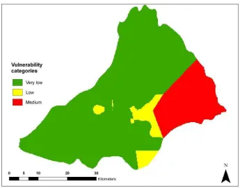
The DRASTIC indices map built following the conventional approach proposed by Aller

et al. (1987), is shown in Figure 19. The highest DRASTIC index determined had a value

of 145, and the lowest was 40. This range was divided into five intervals of equal

magnitude. The zones with greater indices were located within the extreme eastern

mountains and the transition zones between the mountains and the valleys. A great

amount of the total infiltration circulates in this transition zone as mentioned by Ibarra

(2004). This occurred in conjunction with a hydrogeologic zone of higher permeability,

higher recharge rates, less steep slopes, and a lower organic matter content when

vulnerability were located within the valleys of the study area, although these zones

presented the higher nitrate concentrations within the aquifer.

Figure 19. DRASTIC indices vulnerability map.

6.2.Regression results

6.2.1. Ordinary least squares regression results

The ratings used as the input data for all the regressions for the different parameters were

extracted from the corresponding parameter map by using the extract values operation in

ArcGIS/ArcInfo. Sampled sites in which the nitrate concentration exceeded the average

value by two standard deviations were discarded, and thus not included in any of the

regressions. The aquifer media and soil media parameters were not included in the