1
Autocatalytic kinetic model for thermogravimetric analysis and
composition estimation of biomass and polymeric fractions
A. Cabeza, F. Sobrón, F.M. Yedro, and J. García-Serna*
High Pressure Processes Group, Department of Chemical Engineering and
Environmental Tech., University of Valladolid, 47011 Valladolid, Spain
*Corresponding author: Tel.: +34 983184934 E-mail: [email protected] (J. García-Serna)
Abstract
A comprehensive kinetic model of slow pyrolysis of biomass during a Thermogravimetric analysis (TGA) has been developed, including the simulation of variable heating rates, composition estimation and structural analysis of biomass. Biomass was assumed as a matrix of three solid global components (hemicellulose, cellulose and lignin) in which water and oil can be also present.
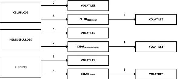
Kinetics were based on an auto-catalytic model because it can simulate the degradation in cellulosic materials, as the cleavage of the biopolymers produce oligomers that accelerate the further depolymerisation. The reaction pathway followed the Waterloo’s mechanism, which stablishes that all solid compounds decompose into volatiles and charcoal. This mechanism was completed by the vaporization of water and oil, and assuming that the formed charcoal can break into volatiles by a slow reaction. The set was solved by the 8th Runge-Kutta’s method and validated by the Simplex Nelder-Mead and Broyden-Fletcher-Goldfarb-Shanno’s methods. The development of this model has a high interest because it can help to understand how the conversion from biomass to biochemicals takes place.
2
samples, also they were perceived between the isothermal and no-isothermal way. On the other hand, an effect of the biomass structure has been reported by the differences between the kinetics of the seeds and of the woody samples. It is remarkable that the developed model could reproduce the cellulose decomposition with a variable heating rate using a unique set of kinetic parameters. This was possible by a no-Arrhenius’ dependence with temperature. In the same way, it was used to predict the initial composition of the studied biomass with deviations lower than 7% for lignin and cellulose.
Keywords: Autocatalytic kinetic, composition estimation, TGA, cellulose, hemicellulose,
lignin.
1. Introduction
The use of fossil fuels as the main raw material for industry is not sustainable, and certainly it will not be the forever-solution. So a new source of basic compounds (i.e. carbon, hydrogen and oxygen) and energy should be considered. This new source could be biomass [1], which can be transformed into bioenergy, biochemical and biofuels in biorefineries [2, 3]. However, the design of these biorefineries requires knowledge about the conversion from raw material to fuels and fast, cheap and accurate biomass-analysing methods. For the latter, several wet methods of chemical analysis have been used [4]. These methods are based on the fractionation of biomass samples and a later isolation of purified fractions, which could be quantified using conventional analytical instruments. Although these techniques have high accuracy and robustness, they are not suitable for an industrial scale because they are expensive and require a lot of time. Another option would be spectroscopic analysis, such as, the Near Infrared Reflectance (NIR) spectroscopy, which reduces time requirements and cost and it is a method with a high reproducibility. Nevertheless, these analysis need data with a very high quality and an initial blank spectrum, which is an important limitation. So, the measurement of the initial biomass composition is an issue that have not an optimal solution yet. Thermogravimetric analysis (TGA) of biomass could be the answer for this problem under certain conditions. In addition, it can provide information about how the thermal decomposition takes place.
3
modelling in the literature. The most extended model considers a first order kinetic for each compound present in biomass assuming that biomass is formed by three main compounds (cellulose, hemicellulose and lignin). These components decompose to charcoal and volatiles by independent reactions. S. Völker [8] used a first order kinetic to adjust the decomposition of pure cellulose and the deviation between the experimental data and the simulation was relatively high. In contrast, Capart R et alt. [9] studied the pure cellulose thermal breaking but considering an autocatalytic model which supposed a good fitting with an overall deviation around 1 %. On the other hand, V. Mangut et al. [10] proposed a kinetic model of nth-order for the degradation of residues from tomato processing industry which could reproduce the biomass behaviour. But A. Zabaniotoua et al. [11], K. Slopiecka et al. [12] and E. Kastanaki et al. [13] studied the TGA kinetics of several lignocellulosic biomass samples, poplar wood and lignite-biomass blends respectively with a first order model and they obtained good fits too. K. Slopiecka et al. and A. Zabaniotoua et al. fitted their TGA as a single compound, which is useful to reproduce the decomposition. However, it is not capable of reproducing the individual behaviour of the biomass components and ensuring that the obtained parameters have physical meaning. On the other hand, E. Kastanaki et al. and V. Mangut et al. adjusted their TGA with individual kinetics for each biomass compound. Therefore, the behaviour of each of them could be simulated and the physical sense of the parameters checked. Nevertheless, they did not studied the causes of the variations in the kinetics of the biomass components assuming that there are no interactions between them. Taking into account this big range of possible models it is difficult to select one because any of them could be a good way to simulate the thermal degradation of biomass. Finally, the autocatalytic model is the option selected in this work due to the fact that it can reproduce the steep changes in cellulosic material better than a first or nth-order model.
4
from the thermogravimetric analysis and from the kinetic parameters fitted previously. This capacity is important because it is a new use for the TGA modelling and, if it is developed correctly, it would become an economic option to obtaining the initial composition of the biomass.
2. Materials and methods
2.1. Materials
Grape seeds from Vitis vinifera L (Tempranillo) from Matarromera S.A. winery (Valbuena de Duero, Spain) campaign 2011 and several woody wastes were used as raw material. Material for this study was ground to a particle size of 0.5-1.0 mm.
The reagents used for HPLC analysis were: cellobiose (+98%), glucose (+99%), fructose (+99%), glyceraldehyde (95%), pyruvaldehyde (40%), arabinose (+99%), 5-hydroxymethylfurfural (99%), lactic acid (85%), formic acid (98%), acrylic acid (99%), mannose (+99%), xylose (+99%) and galactose (+99%) purchased from Sigma and used without further modification. For the structural carbohydrates and lignin determination sulfuric acid (98%) and calcium carbonate (≥ 99.0%) were used as reagents supplied by Sigma too.
2.2. Biomass characterization
2.2.1. Sugar content
The sugar content measurement of a biomass sample requires its hydrothermal fractionation followed by a hydrolysis of the product which will be fed to a HPLC later. The hydrolysis is needed because the fractionation generates a range of polymeric fractions and compounds which could not be directly identified in a HPLC. So they have to be cleavaged by a further hydrolysis into their basic units or monomers, e.g. glucose, fructose, xylose and arabinose.
5
The HPLC column used for the separation of the compounds was a SUGAR SH-1011 Shodex at 50 ºC at a flow of 0.8 ml/min using a solution of 0.01N of sulphuric acid and Milli-Q water as mobile phase. A Waters IR detector 2414 and Waters dual λ absorbance detector 2487 (210 nm and 254 nm) were used to identify the sugars and their derivatives.
2.2.2. Solid analysis. Klason lignin determination and sugars attached to the solid
The raw material and the solid residue generated by the hydrolysis were analysed for lignin content using the Klason assay according to the TAPPI standard method T-222 om-98 [16]. To do so, 300 mg of sample was put into laboratory glass bottles, 3 mL of sulfuric acid (72%) was added and it was incubated during 30 min at 30ºC and it was shaken vigorously every 5-10 min. Then, the mixture was diluted with 84 mL of deionized water and it was placed in an oven for 1 h at 121ºC. At that moment, the sample was taken out from the oven, cooled down to room temperature and the mixture was filtered under vacuum. The obtained solid after filtration was dried at 105ºC for 24 h, it was cooled down in a desiccator and then it was weighted. This solid was introduced in the calcination oven at 550ºC for 24 h to determine the ash content. Considering the weight differences, the Klason lignin content was calculated. The hydrolysis liquid was neutralized with calcium carbonate to pH=6-7, then it was filtered and analysed by HPLC as explained in section 2.3.1.2 Sugars.
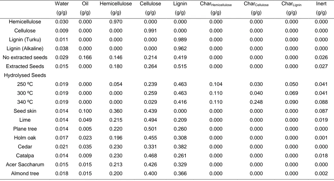
The initial composition calculated by the methods described in 2.2.1 and 2.2.2 is collected in ¡Error! No se encuentra el origen de la referencia..
2.3. Experimental set-up and procedure
TGA were carried out in a TGA/SDTA RSI analyzer of Mettler Toledo. Samples of approximately 10 mg were heated from 50ºC to the required temperature at a rate of 20ºC/min under N2 atmosphere (60 NmL/min flow) to determine the carbonization. The final temperature changed with the type of analysis. If the study was at isothermal conditions it had a value between 150ºC and 350 ºC. However, when it was no isothermal the biomass were heated up to temperatures around 800 ºC.
2.3.1. Procedure for the analysis of the effect of the composition
Thermogravimetric analysis at variable temperature with a heating rate of 20ºC/min of woody samples with different lignin content were fitted. So the difference between the kinetics parameters were used to discover how the composition affects to the thermal degradation. TGA of hemicellulose, cellulose and grape skins, which does not have lignin, at the same heating rate were performed to study this factor too.
6
The effect of the biomass structure was studied comparing the adjusted kinetic parameters obtained from the TGA (with a heating rate of 20ºC/min) of two types of pure lignin: an alkaline lignin and a sample from Turku, Finland. The last one was extracted using a hydrotropic substance, the p-toluene sulfonate. In addition, the deviation of the kinetics parameters between the TGA (heating rate of 20ºC/min) of a sample of grape seeds and grape seeds extracted with a mixture of ethanol/water (70/30) for 1 hour was considered. The kinetics variation between these grape seeds and hydrolysed grape seeds for 1 hour at three different temperatures (250ºC, 300ºC and 340 ºC) and at a heating rate of 20 ºC/min were analysed too.
2.3.3. Procedure for the analysis of the effect of the heating rate
The role of the heating rate was considered by fitting TGA of pure cellulose at three different heating rate: 5ºC, 10ºC, 20ºC and comparing the values of their kinetics parameters.
2.3.4. Procedure for the analysis of the effect of the isothermal conditions
This factor was studied by the adjustment of the TGA of Acer Saccharum, a type of maple, at 5 temperatures (150ºC, 200ºC, 250ºC, 300ºC and 350ºC) with a heating rate of 20 ºC/min and considering the modifications in the kinetics.
3. Mathematical model
3.1. Biomass composition
7
Simplifying the raw biomass structure we can consider that the cellulose microfibers are connected by hemicellulose in 3D structure of lignin that encloses and protects them (Figure 1). The structure of the biopolymer fractions and other kinds biomass lignin-lean can be a bit different.
Figure 1 HERE
Table 1: HERE
3.2. Reaction pathway
Degradation process
The thermal degradation of biomass in an inert atmosphere (slow pyrolysis conditions) starts with the vaporization of liquid phases. Water evaporates near 100ºC and oil between 100ºC and 300ºC. In this research, we intentionally did not dry the biomass until full dryness to mimic as much as possible some kind of humid conditions and therefore the water evaporation.
At 200ºC lignin begins its decomposition, breaking its weaker parts and enhancing the reaction of hemicellulose and cellulose. Between 250ºC and 275ºC hemicellulose reacts and around 300 ºC it disappears completely, which promotes the cellulose breaking. The last one commences its degradation between 300ºC and 350ºC and, from this point, only lignin, inert substances and the product from the decomposition (charcoal) remains in the biomass. Lignin depletes at 500ºC and charcoal continues in the sample with a very low degradation rate. Charcoal only fades completely if the atmosphere is changed to an oxidant compound.
Reaction mechanism
8
better further prediction. The pathway was completed adding the decomposition of each charcoal to volatiles and with the vaporization of liquid phases if present.
Figure 2: HERE
3.3. The model
Assumptions
Aimed at simplifying the modelling problem it was assumed that:
a. All the reactions are irreversible and independent. So, the degradation kinetics of each component only depend on their composition and temperature [10, 12, 13].
b. There are no energy transport limitations within the biomass particles (as only 10 mg of micronized particles were used for the TGA analysis). Consequently, all the parts of the biomass are at the same temperature.
c. Diffusional mass transport resistances for liquid phases are negligible, as the particles were micronized.
Mass balances
The model of the decomposition process considered a non-stationary mass balance for each component in the biomass sample:
𝑑𝑚𝑗
𝑑𝑡 = 𝑟𝑗= ∑ 𝑔𝑖𝑗· 𝑟𝑖
𝑁𝑟
𝑖=1
( 1 )
And the total variation of mass was calculated by the addition of all of them:
𝑑𝑀
𝑑𝑡 = ∑
𝑑𝑚𝑗 𝑑𝑡
𝑁
𝑗=1
( 2 )
Kinetics
Mass variation was caused by two different phenomena: reaction kinetics for the solid material and mass transfer of the liquid phases.
9
Mass transfer of liquid phases was described by the partial mass transfer coefficient in the gas phase, the mass transfer area and the difference between de equilibrium concentration in the liquid phase and the global concentration in the gas phase (as driving force) ( 3 ).
𝑟𝑖 = ℎ · 𝑆 · (𝐶𝑗∗− 𝐶𝑗) ( 3 )
As the operating pressure is the atmospheric, the equilibrium concentration ( 4 ) was obtained by the ideal gas equation and the vapour pressure calculated by the Antoine equation ( 5 ) of each compound. The Antoine’s equation coefficients of each liquid phase are compiled in Table 2.
𝐶𝑗∗= 𝑃𝑗∗
𝑅 · 𝑇 ( 4 )
ln(𝑃𝑗∗) = Aj+
𝐵𝑗
𝐶𝑗+ 𝑇+ 𝐷𝑗· ln(𝑇) + 𝐸𝑗· 𝑇
𝐹𝑗 ( 5 )
Table 2: HERE
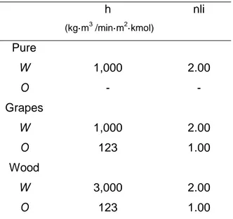
In addition, the transfer area was considered as a function of the mass in the solid, so the final expression for the mass transfer was:
𝑟𝑖 = ℎ · (𝐶𝑗∗) · 𝑚𝑗𝑛𝑙𝑖 ( 6 )
Solid kinetics: for solid organic compounds
As it was mentioned in the introductory section, there are two options for temperature dependent kinetics, i.e. a first order reaction ( 7 ) and an autocatalytic reaction ( 8 ). The first is the most extended option in the bibliography [9-13] and the second is proposed because its response is very similar to the behaviour of the biomass observed in the literature [9] and in previous studies. Both kinetic equations considered an Arrhenius’ dependence with temperature.
𝑟𝑖 = 𝑘𝑖· 𝑚𝑖 = 𝑘𝑜𝑖· 𝑒
−𝐸𝑅·𝑇𝑎𝑖 · 𝑚
10
𝑟𝑖= 𝑘𝑜𝑖· 𝑒
−𝑅·𝑇𝐸𝑎𝑖 · 𝑚
𝑗𝑛𝑖· (1 − 𝛼𝑖· 𝑚𝑗)𝛽𝑖 ( 8 )
The coefficient 𝛼𝑖 is the initialization factor which indicates the resistance of the biomass against the degradation. It is used to establish the initial value of the reaction velocity. In this work 𝛼𝑖 was fixed at 0.99, as it is the most recurrent value in the literature [9]. The coefficient 𝛽𝑖 is the acceleration factor and represents how fast the degradation is once it has started. The autocatalytic kinetics can predict the dramatic changes in the total mass along with temperature better than a first order kinetics. In view of that, autocatalytic kinetics was the selected option for this work.
In addition, as pure cellulose has been studied at different rates of heating a non-Arrhenius’ dependence with the temperature was added to equation ( 9 ) for this compound. Therefore, the decomposition of cellulose was simulated by equation ( 10 ). This other kind of reaction rate expression was needed because the biomass shows a different behaviour when the heating rate varies along with time (or temperature), as the polymeric structure can both collapse or swell [8, 9, 14, 15]. The parameter “c” is a correction factor to the cellulose decomposition when a variable heating rate is used. Nevertheless, we assumed that it could be affected by the biomass structure and heating process too. For this reason, three sets of “c” values are present in ¡Error! No se encuentra el origen de la referencia..
𝑟𝑖 = 𝑘𝑜𝑖· 𝑒
−𝑅·𝑇+𝑐·𝑇+ln(𝑇)𝐸𝑎𝑖 · 𝑚
𝑗𝑛𝑖· (1 − 𝛼𝑖· 𝑚𝑗)𝛽𝑖
( 11 )
3.4. Resolution
The system of 8 ordinary differential equations (ODE) that results from the model was solved by the Runge-Kutta’s method with 8th order of convergence [18]. The validation of the model with the experimental data was done applying the Simplex Nelder-Mead method for obtaining an initial estimation of the parameters together with the Broyden-Fletcher-Goldfarb-Shanno’s method to improve this initial solution [18]. During the optimization, the optimization range were selected in order to achieve an optimum which would have physical meaning.
11
𝐴𝐴𝐷 = ∑|𝑥𝑖𝐸𝑋𝑃− 𝑥𝑖𝑆𝐼𝑀| 𝑥𝑖𝐸𝑋𝑃
𝑁
𝑖=1
· 100 ( 10 )
The developed program is available for free in the web page of the research group of high pressure processes of the University of Valladolid (http://hpp.uva.es/software/).
4. Results and discussion
4.1. Pure samples
This adjustment was done taking into account the theoretical development showed in section 3. The initial composition of each compound is arrayed in ¡Error! No se
encuentra el origen de la referencia..
4.1.1. Hemicellulose
The fitting of pure hemicellulose decomposition (with an average absolute deviation of 2.2%) is shown in Figure 3 and the kinetic parameters in ¡Error! No se encuentra el origen de la referencia.. The mass transfer parameters were averaged for all the samples (complex samples too) and are shown in Table 3.
Table 3: HERE
12
As we can see in Figure 3, the proposed model can simulate the degradation of the biomass components. This simulation of each component is a good tool due to the fact that it provides a way to ensure that the simulation has a physical sense. Thus, it can be easily checked if each individual behaviour agrees with the experimental data.
Figure 3: Fitting for the hemicellulose decomposition with a heating rate of 20 ºC/min. W: Water. HC: Hemicellulose. XHC: Char of hemicellulose.TOTAL: Simulated TGA. EXP: Experimental TGA.
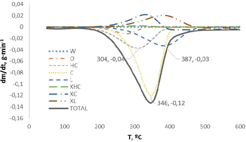
This analysis was completed with the simulated differential thermography (DTG) showed in Figure 4. It can be seen that there is a first minimum at 90 ºC corresponding to the first slope change at 50 ºC in Figure 3 due to water evaporation. The second minimum, which appears at 346ºC, is related with hemicellulose decomposition and it originates the second change in slope at 250ºC. Furthermore, there is a maximum at 370 ºC which represents the charcoal formation and implies the change in slope at 401ºC. The combination (by addition) of all of these peaks gives a minimum at 362ºC which is the representative temperature of hemicellulose thermal degradation. This value does not agree with other authors. For example, Elyounssi, K. et alt. [14] and Slopiecka, K. [12] found that this peak is between 260-299 ºC at low heating rates and Williams, P. T. and Besler, S. [5] discovered that it is around 310ºC at 20K/min. This decoupling could be caused by the fact that the value obtained in this work is for extracted hemicellulose and the others from complex samples. However, the temperature of the hemicellulose maximum in our woody biomass fittings (304ºC) agrees with the value of these authors (
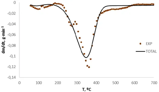
Figure 5). So, this deviation would show that the same compound in a different structure has a different behaviour against thermal degradation. Finally, the comparison between experimental and simulated DTG were done (Figure 6). Both curves presents the same behaviour, with the main variations at the same temperatures. The differences between them could come from the numerical evaluation of the experimental derivative, which is obtained by a central difference approximation.
Figure 4: HERE
Figure 5: HERE
Figure 6: HERE
13
The adjustment of the TGA of cellulose at heating rates of 20ºC/min (average absolute deviation of 6.6%), 10ºC/min (average absolute deviation of 3.7%) and 5ºC/min (average absolute deviation of 1.2%) was done in this point. The obtained kinetic parameters are presented in ¡Error! No se encuentra el origen de la referencia.. The thermolysis process started at 300ºC, with the fractionation of cellulose, and continued until 400ºC. After this temperature, there was only charcoal in the sample. This experimental behaviour of cellulose agrees with the work of previous authors [4, 5, 7, 9, 11, 12] and it could be simulated using the same set of kinetics parameter for the three experiments.
A decoupling was observed in mass variation originated by the different heating rates: the lower the heating rate is, the higher yield of charcoal is obtained. The origin of this fluctuation could be that a slow heating rate provides enough time to appear secondary reactions which increase the charcoal production [9, 14, 15] due the collapse of the polymeric structure. For this reason, a specified model was proposed to cellulose decomposition (point 3.3). The idea was to represent this change in the decomposition process by a non-Arrhenius’ dependence with temperature.
It is observed by the differential thermography of cellulose that its pure fraction shows a peak at 370ºC. Again, it decreased to 346ºC in a woody sample (
Figure 5). This last value is similar to the data provided by Williams, P. T. and Besler, S. [5] and Carrier et al [4]. Consequently, there is a modification in the thermal degradation of the cellulose when it is inside a complex sample due to the variation in structure.
4.1.3. Lignin
14
The differential thermogravimetric analysis of the lignin showed a minimum at 322ºC for its isolated fraction. This value was far from the value of 387ºC, that appeared in a woody sample (
Figure 5) and from the value established by Williams, P. T. and Besler, S. [5] (390ºC) or Carrier et al [4] (395ºC). This decoupling would be again caused by an effect of the structure of the sample.
4.2. Complex samples
In this section the TGA of complex samples was studied. The procedure was to try to simulate the experimental data from the TGA of complex samples with the kinetics parameters obtained for the pure fractions. Hence, only if this simulation had no correlation with the experimental performance, a new set of parameters would be searched.
4.2.1. Grape seeds
This section is focused in the TGA of wastes from the wine industry: seeds, extracted seeds, seed skins and hydrolysed seeds.
4.2.1.1. No-extracted seeds and extracted seeds
The TGA of the no-extracted seeds was fitted (average absolute deviation of 1.6%) using the same kinetics parameters for the pure hemicellulose and cellulose and changing the parameters related with the lignin. This change implies that a relation between the three main components exit and justified the necessity of use a kinetic more complex than a first order kinetic to model the system. The used reaction pathway was the same as in pure samples.
15 Figure 7: HERE
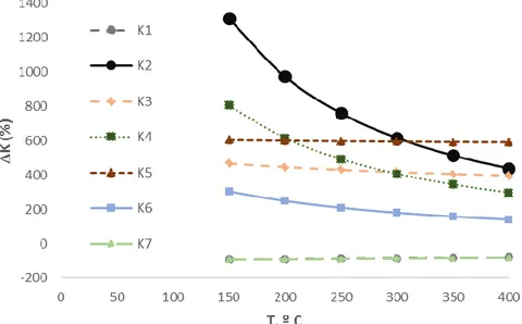
It is shown in Figure 7 that the reactions more affected by the extraction are the degradation of the hemicellulose (K1 and K7) and lignin (K3, K4 and K5). Cellulose (K2 and K6) decomposition is also increased but around 50% less. These results would be coherent with the expected behaviour due to the fact that lignin encloses cellulose and hemicellulose and it would be the most exposed. Regarding hemicellulose, it was expected that this process enhance its thermal breaking because it is water soluble. K8 and K9 (kinetic constant of cellulose and hemicellulose char degradation to volatiles respectively) were not affected. This result could be explained because the main contribution to the char comes from the lignin. It is also interesting the fact that the higher the degradation temperature is, the lower effect has the pre-treatment. Which would be expected because temperature enhances exponentially thermal degradation.
4.2.1.2. Grape skin
The main characteristic of this sample is that it does not have lignin. For this reason, the model had to reproduce the experimental behaviour using only the parameters related with hemicellulose and cellulose (¡Error! No se encuentra el origen de la referencia.). The model represents well the process (average absolute deviation of 1.9%) but there is a dramatic change of slope at 275ºC that cannot simulate. In addition, it needed a change in the kinetics parameters which could be explained again by the effect of the biomass structure.
4.2.1.3. Hydrolyzed samples
As we mentioned before, the grape seeds suffered for 1 hour three different hydrolysis process at temperatures of 250ºC, 300ºC and 340ºC. The result was a substance partially degraded with high content of charcoal. These three degraded samples were used in a TGA whose results were fitted with only a set of parameters (¡Error! No se encuentra el origen de la referencia.) with an average absolute deviation of 1.1% at 250 ºC, 0.86% at 300ºC and 0.68% at 340ºC. This previous degradation generates a material which higher resistance against thermal degradation due to the fact that some charcoal was formed. This statement is shown in Figure 8, where the variation is
defined by the following mathematical
16
kinetics decrease respect the non-treated samples. However, hemicellulose kinetics presents the opposite behaviour but it is not representative because the main part of hemicellulose disappear during the hydrolysis.
Figure 8: HERE
The lignin kinetic variations observed in Figure 8 could be justified again with its protection function like in part 4.2.1.1. On the other hand, cellulose shows in this case a higher modification in kinetics due to their degradation during the hydrolysis. Finally, temperature reduce again the differences between the thermal degradation of both samples. K8 and K9 do not appear because of their low contribution to the total char.
4.2.2. Woody biomass
In this point, the thermal decomposition in isothermal and no isothermal conditions of woody biomass is considered. All the fittings needed a modification in the kinetics parameters.
4.2.2.1. Non-isothermal process
17 Table 4: HERE
Figure 9: HERE
It is remarkable that kinetic constants related with hemicellulose degradation do no change their values (for this reason they are not present in Figure 9). This result could be explained by the fact that in this study case there were not previous factors that can solve it. So, its interactions with cellulose and lignin would be independent to the lignin concentration. The role of the temperature is the same as in parts 4.2.1.1 and 4.2.1.3 and K8 is not represented because there is no change in its value.
4.2.2.2. Isothermal process
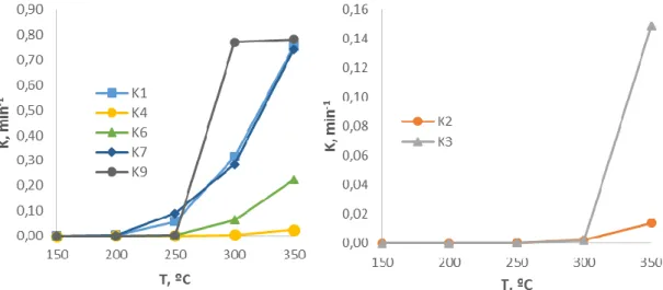
Finally, the TGA of a sample of Acer Saccharum was studied in isothermal conditions at 150, 200, 250, 300 and 350 ºC. The adjustment needed a set of parameters for each temperature, when it is higher than 200ºC, and different from the parameters used in the non-isothermal process (¡Error! No se encuentra el origen de la referencia.). Their average absolute deviations were: 0.71%, 0.70%, 0.39%, 0.63% and 2.68% respectively. This discrepancy between the kinetics due to the type of process could be caused by a protective interaction between species. This means that, in an isothermal mode, the decomposition is low up to a certain temperature is reached (250ºC) and hemicellulose degradation starts enhancing the decomposition of cellulose and lignin. Besides, there is an enhanced in lignin degradation 300 ºC, when cellulose would start its degradation. This idea could explain the drastic change in the kinetics constants shown in Figure 10 at 250ºC and 300ºC.
Figure 10: HERE
It can be seen in Figure 10 that the thermal degradation at isothermal conditions depends on temperature strongly (as it was expected). In this case K5 and K8 are not present in the graph, because they did not change. This would be caused by the fact that the maximum operational temperature (350ºC) is not high enough to break lignin or cellulose char.
18
Once all the experimental data have been adjusted, the capability of the model to estimate the initial composition of the biomass was tested. The sample used to try this estimation was the TGA of non-extracted grape seeds.
The prediction implies an optimization problem in which the difference between the experimental and simulated TGA must be minimized changing the values of the initial composition ( 12 ). The problem was limited by the following restraints. It was assumed that there is not initial charcoal in the sample and that the initial composition of water, oil, hemicellulose, cellulose and lignin were in the ranges showed in the
Table 5. The amount of inert compounds was obtained by balance to the total.
min
𝑚𝑗 ( ∑ |𝑀𝐸𝑥𝑝− 𝑀|
𝑡=𝑡𝑓
𝑡=0
) ;𝑚𝑗𝑚𝑖𝑛 < 𝑚𝑗 < 𝑚𝑗𝑚𝑎𝑥; 𝑗 ∈ [1, 𝑁] ( 12
)
Table 5: HERE
The calculated composition is not very accurate because in some compounds the deviation is high, for example the maximum deviation for water was 60.5 % (Table 6). But taking into account that the values for the maximum and the minimum of each component were stablished in a general way, the prediction is good enough. In order to improve these values, more experimental compositions would be needed to fix a better optimization range. It is interesting that the calculated cellulose composition is closer to the experimental one than the hemicellulose composition. This result could be caused by the fact that the oil vaporization and hemicellulose degradation can appear both between 250ºC and 300ºC.
Table 6: HERE
5. Conclusions
19
too. In addition, the model can reproduce the effect of the heating rate in the decomposition using a non-Arrhenius’ dependence with the temperature. Due to the fact that the kinetics parameters change with the type of biomass it is deduced that the structure of biomass has a very important role in thermal degradation. Also important is the composition because some species can work as a shield that avoids the degradation of the others until their cleavage start. Finally, a preliminary composition estimation were done, starting from a TGA curve and estimating the composition of the biomass material. This prediction has an acceptable accuracy especially for cellulose and lignin (differences lower than 7%). However, the prediction of the essential oil is trick and in order to increase model fidelity, more experiments would be needed, which would allow to stablish better limits for the optimization ranges of the initial composition and to improve the kinetics parameters.
T
Table 7: HERE
Acknowledgements
The authors acknowledge the Spanish Economy and Competitiveness Ministry, Project Reference: ENE2012-33613 and the regional government (Junta de Castilla y León), Project Reference: VA330U13 for funding. The authors would like to thank Prof. Pedro Fardim and Dr. Konstantin Gabov from Åbo Akademi for their help with the hydrotropic lignin.
Nomenclature
Acronyms
C: Cellulose. HC: Hemicellulose. L: Lignin.
O: Oil.
TGA: Thermogravimetric analysis. W: Water.
20 Subindex and superindex
EXP: Experimental data of the TGA. in: inert compounds.
TOTAL: Total simulated TGA.
Greek letters and symbols
𝛼𝑖: Initialization factor, adim.
𝛽𝑖: Acceleration factor, adim.
𝐴𝑗− 𝐹𝑗: Antoine’s equation coefficients of the compound “j”, adim.
𝑐: Correction factor for the kinetic in the decomposition at different heating rates of the cellulose, adim.
𝐶𝑗: Concentration of “j” in the gas phase, kmol/m3.
𝐶𝑗∗: Equilibrium concentration of “j” in the interphase between the liquid and the gas
phase, kmol/m3.
𝐸𝑎𝑖
𝑅: Activation energy of the reaction “i”, K.
ℎ: Partial mass transfer coefficient between the liquid and the gas, kgj· m3 /min·m2·kmolj.
𝑘𝑜𝑖: Preexponential factor for the reaction “i”, min
-1.
𝑘𝑖: Kinetic constant for the reaction “i”, min-1.
𝑀𝑒𝑥𝑝: Experimental mass fraction of unreacted biomass, gsample/gsample initial.
𝑀: Mass fraction of unreacted biomass, gsample/gsample initial.
𝑚𝑗𝑚𝑎𝑥: Maximun value for mass fraction of the compound “j” in the biomass, g/g.
𝑚𝑗𝑚𝑖𝑛: Minimum value for mass fraction of the compound “j” in the biomass, g/g.
𝑚𝑗: Mass fraction of the compound “j” in the biomass, g/g.
𝑁: Number of compounds in the biomass, adim.
𝑛𝑖: order of reaction of the reaction “i”, adim.
𝑛𝑙𝑖: Mass transfer order, adim.
𝑁𝑟: Number of reactions, adim.ç
𝑃𝑗∗: Vapour pressure of the compound “j”, atm.
𝑟𝑖: Reaction velocity number “i”, g/min·g.
𝑟𝑗: Reaction velocity of decomposition for the component “j” in the biomass, g/min·g.
𝑆: Exchange surface between the liquid and the gas, m2.
t: Operating time, min.
21
𝒙𝒊𝒆𝒙𝒑: Experimental biomass fraction, gsample/gsample initial.
𝒙𝒊𝑺𝑰𝑴: Simulated biomass fraction, gsample/gsample initial.
List of figures
Figure 1: Schema of the biomass structure.
Figure 2: Reaction pathway in a thermal decomposition.
Figure 3: Fitting for the hemicellulose decomposition with a heating rate of 20 ºC/min. W: Water. HC: Hemicellulose. XHC: Char of hemicellulose.TOTAL: Simulated TGA. EXP: Experimental TGA.
Figure 4: Simulated differential thermography of the hemicellulose TGA. W: Water. HC: Hemicellulose. XHC: Char of hemicellulose. TOTAL: Simulated DTG.
Figure 5: Simulated differential thermography of the lime TGA. W: Water. HC: Hemicellulose. XHC: Char of hemicellulose. TOTAL: Simulated DTG. O: Oil. C: Cellulose. L: Lignin. XC: Char of cellulose. XL: Char of lignin.
Figure 6: Simulated differential thermography and experimental differential thermography. EXP: Experimental DTG. TOTAL: Simulated DTG.
Figure 7: Variation of the kinetic constants between the extracted seeds and the no extracted seeds. K1: kinetic constant of hemicellulose degradation to volatiles. K2: kinetic constant of cellulose degradation to volatiles. K3: kinetic constant of lignin degradation to volatiles. K4: kinetic constant of lignin degradation to char. K5: kinetic constant of lignin char degradation to volatiles. K6: kinetic constant of cellulose degradation to char. K7: kinetic constant of hemicellulose degradation to char.
22
Figure 9: Variation in percentage of the reaction kinetics between the samples between 26% and 30% of lignin. K2: kinetic constant of cellulose degradation to volatiles. K3: kinetic constant of lignin degradation to volatiles. K4: kinetic constant of lignin degradation to char. K5: kinetic constant of lignin char degradation to volatiles. K6: kinetic constant of cellulose degradation to char.
Figure 10: Kinetics constant in each isothermal process.K1: kinetic constant of hemicellulose degradation to volatiles. K2: kinetic constant of cellulose degradation to volatiles. K3: kinetic constant of lignin degradation to volatiles. K4: kinetic constant of lignin degradation to char. K6: kinetic constant of cellulose degradation to char. K7: kinetic constant of hemicellulose degradation to char. K9: kinetic constant of hemicellulose char degradation to volatiles.
List of tables
Table 1: Initial composition of the samples.
Table 2: Antoine’s equation coefficients of water (W) and oil (O).
Table 3: Averaged mass transfer parameters of water (W) and oil (O).
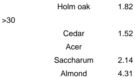
Table 4: Groups of woody samples taking into account its lignin content.
Table 5: Initial composition variation ranges for the composition estimation of no-extracted grape seeds.
Table 6: Comparison between the estimated and experimental composition of no-extracted grape seeds.
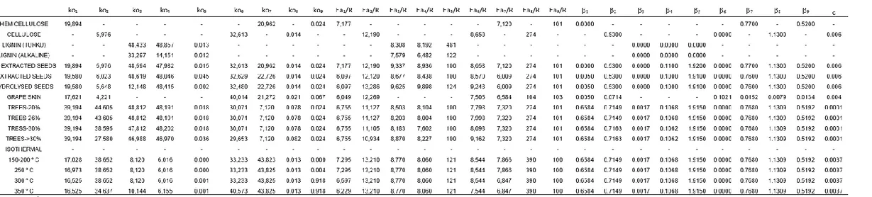
Table 7: Kinetics parameters fitted for all the samples.
23
[1] Clark JH, Budarin V, Deswarte FEI, Hardy JJE, Kerton FM, Hunt AJ, et al.
Green chemistry and the biorefinery: A partnership for a sustainable future.
Green Chemistry. 2006;8:853-60.
[2] Bozell JJ. Feedstocks for the future - Biorefinery production of chemicals
from renewable carbon. Clean - Soil, Air, Water. 2008;36:641-7.
[3] Cheng S, Zhu S. Lignocellulosic feedstock biorefinery-the future of the
chemical and energy industry. BioResources. 2009;4:456-7.
[4] Carrier M, Loppinet-Serani A, Denux D, Lasnier J-M, Ham-Pichavant F,
Cansell F, et al. Thermogravimetric analysis as a new method to determine the
lignocellulosic composition of biomass. Biomass and Bioenergy.
2011;35:298-307.
[5] Williams PT, Besler S. The Influence of Temperature and Heating Rate on
the Slow Pyrolysis of Biomass. Renewable Energy. 1996;7:233-50.
[6] Lv D, Xu M, Liu X, Zhan Z, Li Z, Yao H. Effect of cellulose, lignin, alkali and
alkaline earth metallic species on biomass pyrolysis and gasification. Fuel
Processing Technology. 2010;91:903-9.
[7] Chen Q, Zhou JS, Liu BJ, Mei QF, Luo ZY. Influence of torrefaction
pretreatment on biomass gasification technology. Chinese Science Bulletin.
2011;56:1449-56.
[8] S. Völker TR. Thermokinetic investigation of cellulose pyrolysis. Impact of
initial and final mass of kinetics results. Journal of Analytical and Applied
Pyrolysis. 2002;62:165-77.
[9] Capart R, Khezami L, Burnham AK. Assessment of various kinetic models
for the pyrolysis of a microgranular cellulose. Thermochimica Acta.
2004;417:79-89.
[10] Mangut V, Sabio E, Gañán J, González JF, Ramiro A, González CM, et al.
Thermogravimetric study of the pyrolysis of biomass residues from tomato
processing industry. Fuel Processing Technology. 2006;87:109-15.
[11] Zabaniotou A, Ioannidou O, Antonakou E, Lappas A. Experimental study of
pyrolysis for potential energy, hydrogen and carbon material production from
lignocellulosic
biomass.
International
Journal
of
Hydrogen
Energy.
2008;33:2433-44.
[12] Slopiecka K, Bartocci P, Fantozzi F. Thermogravimetric analysis and kinetic
study of poplar wood pyrolysis. Applied Energy. 2012;97:491-7.
[13] Kastanaki E, Vamvuka D, Grammelis P, Kakaras E. Thermogravimetric
studies of the behavior of lignite–biomass blends during devolatilization. Fuel
Processing Technology. 2002;77–78:159-66.
[14] Elyounssi K, Collard FX, Mateke JAN, Blin J. Improvement of charcoal yield
by two-step pyrolysis on eucalyptus wood: A thermogravimetric study. Fuel.
2012;96:161-7.
[15] Van de Velden M, Baeyens, J., Brems, A., Janssens, B., Dewil, R.
Fundamentals, kinetics and endothermicity of the biomass pyrolysis reaction.
Renewable Energy. 2010;35:232-42.
[16] Meng LY, Kang SM, Zhang XM, Wu YY, Xu F, Sun RC. Fractional
pretreatment of hybrid poplar for accelerated enzymatic hydrolysis:
Characterization of cellulose-enriched fraction. Bioresource Technology.
2012;110:308-13
24
25
Figure 1: Schema of the biomass structure.
CELULLOSE
HEMICELLULOSE
LIGNING
2
VOLATILES
6
CHARCELULLOSE
1
VOLATILES
7
CHARHEMICELULLOSE
3
VOLATILES
4
CHARLIGNIN
8
VOLATILES
9
VOLATILES
5
VOLATILES
26
Figure 3: Fitting for the hemicellulose decomposition with a heating rate of 20 ºC/min. W: Water. HC: Hemicellulose. XHC: Char of hemicellulose.TOTAL: Simulated TGA.
EXP: Experimental TGA.
Figure 4: Simulated differential thermography of the hemicellulose TGA. W: Water. HC:
Hemicellulose. XHC: Char of hemicellulose. TOTAL: Simulated DTG.
Figure 5: Simulated differential thermography of the lime TGA. W: Water. HC:
Hemicellulose. XHC: Char of hemicellulose. TOTAL: Simulated DTG. O: Oil. C:
27
Figure 6: Simulated differential thermography and experimental differential thermography. EXP: Experimental DTG. TOTAL: Simulated DTG.
Figure 7: Variation of the kinetic constants between the extracted seeds and the no extracted seeds. K1: kinetic constant of hemicellulose degradation to volatiles. K2:
kinetic constant of cellulose degradation to volatiles. K3: kinetic constant of lignin degradation to volatiles. K4: kinetic constant of lignin degradation to char. K5: kinetic
28
Figure 8: Variation of the kinetic constantan between the hydrolysed seeds and the non- hydrolysed seeds. K1: kinetic constant of hemicellulose degradation to volatiles. K2: kinetic constant of cellulose degradation to volatiles. K3: kinetic constant of lignin degradation to volatiles. K4: kinetic constant of lignin degradation to char. K5: kinetic
constant of lignin char degradation to volatiles. K6: kinetic constant of cellulose degradation to char. K7: kinetic constant of hemicellulose degradation to char.
Figure 9: Variation in percentage of the reaction kinetics between the samples between 26% and 30% of lignin. K2: kinetic constant of cellulose degradation to volatiles. K3:
kinetic constant of lignin degradation to volatiles. K4: kinetic constant of lignin degradation to char. K5: kinetic constant of lignin char degradation to volatiles. K6:
29
Figure 10: Kinetics constant in each isothermal process.K1: kinetic constant of hemicellulose degradation to volatiles. K2: kinetic constant of cellulose degradation to
volatiles. K3: kinetic constant of lignin degradation to volatiles. K4: kinetic constant of lignin degradation to char. K6: kinetic constant of cellulose degradation to char. K7:
Table 1: Initial composition of the samples. 1
Water (g/g)
Oil (g/g)
Hemicellulose (g/g)
Cellulose (g/g)
Lignin (g/g)
CharHemicellulose (g/g)
CharCellulose (g/g)
CharLignin (g/g)
Inert (g/g)
Hemicellulose 0.030 0.000 0.970 0.000 0.000 0.000 0.000 0.000 0.000
Cellulose 0.009 0.000 0.000 0.991 0.000 0.000 0.000 0.000 0.000
Lignin (Turku) 0.011 0.000 0.000 0.000 0.989 0.000 0.000 0.000 0.000
Lignin (Alkaline) 0.038 0.000 0.000 0.000 0.962 0.000 0.000 0.000 0.000
No extracted seeds 0.029 0.166 0.146 0.214 0.419 0.000 0.000 0.000 0.026
Extracted Seeds 0.015 0.000 0.180 0.264 0.515 0.000 0.000 0.000 0.027
Hydrolysed Seeds
250 ºC 0.019 0.000 0.054 0.239 0.463 0.104 0.030 0.050 0.041
300 ºC 0.019 0.000 0.000 0.259 0.463 0.110 0.040 0.069 0.041
340 ºC 0.019 0.000 0.000 0.029 0.416 0.110 0.248 0.090 0.088
Seed skin 0.014 0.100 0.360 0.439 0.000 0.000 0.000 0.000 0.087
Lime 0.014 0.049 0.215 0.494 0.209 0.000 0.000 0.000 0.019
Plane tree 0.014 0.005 0.220 0.501 0.260 0.000 0.000 0.000 0.000
Holm oak 0.017 0.023 0.196 0.455 0.308 0.000 0.000 0.000 0.001
Cedar 0.021 0.035 0.230 0.331 0.382 0.000 0.000 0.000 0.000
Catalpa 0.014 0.009 0.230 0.468 0.261 0.000 0.000 0.000 0.018
Acer Saccharum 0.015 0.015 0.213 0.426 0.329 0.000 0.000 0.000 0.000
31
Table 2: Antoine’s equation coefficients of water (W) and oil (O).
W O
Aj 6.21E+01 1.22E+01 Bj -7.26E+03 5.88E+03 Cj 0.00E+00 -2.93E+02 Dj 7.30E+00 0.00E+00 Ej 4.17E-06 0.00E+00 Fj 1.00E-02 0.00E+00
Table 3: Averaged mass transfer parameters of water (W) and oil (O).
h
(kg·m3 /min·m2·kmol)
nli
Pure
W 1,000 2.00
O - -
Grapes
W 1,000 2.00
O 123 1.00
Wood
W 3,000 2.00
O 123 1.00
Table 4: Groups of woody samples taking into account its lignin content.
Lignin content
(wt%)
Samples A.A.D. a
(%)
20
Lime 1.97
26
Plane tree 1.46
Catalpa 1.87
32
Holm oak 1.82 >30
Cedar 1.52
Acer
Saccharum 2.14
Almond 4.31
a Average absolute deviation between experimental and simulated data.
Table 8: Initial composition variation ranges for the composition estimation of no-extracted grape seeds.
mmina (g/g)
mmaxb (g/g)
Wc 0.00 0.08
Od 0.00 0.20
HCe 0.10 0.25
Cf 0.15 0.60
Lg 0.15 0.45
a
The lowest mass fraction in the optimization. b
The highest mass fraction in the optimization. c Water content. d Oil content . e Hemicellulose content. f cellulose content . g lignin content .
Table 9: Comparison between the estimated and experimental composition of
no-extracted grape seeds.
Wa Ob HCc Cd Le inf
m (wt%)g
Experimental 0.0292 0.1655 0.1461 0.2142 0.4187 0.0263
Estimated 0.0469 0.1149 0.1887 0.2215 0.4121 0.0159
Deviation (%)h 60.5% -30.6% 29.2% 3.39% -1.57% -39.5%
a
Water. b Oil. c Hemicellulose. d Cellulose. e Lignin. f Inert. g Biomass composition in weight percentage. h Deviation between the estimated and real composition.
Table 7: Kinetics parameters fitted for all the samples 2
3