Effluents characterization using NIR and UV Vis spectroscopy

CHEMICAL ENGINEERING

UNIVERSIDAD DE VALLADOLID

Effluents characterization using NIR and UV-Vis

spectroscopy

MIGUEL PERLINES SÁNCHEZ

TÍTULO: Effluents characterization using NIR and UV-Vis

ALUMNO: Miguel Perlines Sánchez

FECHA: MARZO 2014

CENTRO: Universidade do Minho

TUTOR: Eugénio Ferreira

CALIFICACIÓN LOCAL:

CALIFICACIÓN UVA:

Valladolid 6 de marzo de 2014

Coordinador Sócrates

Fdo: Rafael Mato Chaín

INGENIERÍA QUÍMICA

UNIVERSIDAD DE VALLADOLID

PROYECTO FIN DE CARRERA

PEDRO GARCÍA ENCINA, coordinator of Departamento

de Ingeniería Química de la Universidad de Valladolid, CERTIFY:

This PROJECT has done under supervision of Doctor Eugénio

Ferreira and Doctor Daniela Mesquita, in Universidade do Minho

and it is entitled: Effluents characterization using NIR and UV-Vis

spectroscopy.

Valladolid, 06 March 2014

Fdo. Pedro García Encina

S

Nitrogen compounds (e.g. nitrates - NO3-) discharge into the environment can cause

serious problems such as eutrophication and deterioration of water courses. The biological nitrate reduction, named denitrification, has been shown to be more useful, economical, and the most versatile approach among all methods to remove nitrate from wastewaters. To prevent imbalances of those biological processes, analytical methods with chemicals addition are routinely used for systems monitoring. The search for a rapid technique could be an alternative monitoring procedure to enhance the process performance.

Over the last thirty years, the application of spectroscopy techniques for industrial process monitoring is achieving an increasing significance. This technology has been mostly applied in the food industry and in the pharmaceutical industry. Regarding environmental processes, the application of spectroscopy is still rarely applied. In this work, UV-Visible and Near-Infrared (NIR) spectroscopy techniques were used to monitor denitrifying processes using different carbon sources: acetate, propionate (volatile fatty acids - VFAs), glucose, and sucrose (sugars). Denitrifying rates were also found using four different biomass/chemical oxygen demand (VSS/COD) ratios. The main goal of this project was to test the ability of each spectroscopy technique to detect and monitor the denitrification process. For each assay, nitrate and each carbon source were also analyzed using standard analytical methods. Using spectral data and chemometrics tools, models for different parameters were developed: nitrate, VFAs, and sugars. After spectra pre-processing for removing the less relevant information and with application of partial least squares regression (PLS) the described parameters were modeled.

After the evaluation of specific consumption rates, it was concluded that acetate was the best carbon source in denitrifying conditions. Considering the VSS/COD ratios analyzed, VSS/COD ratio of 0.1 provided the best overall results.

Regarding UV-Visible spectral data, the estimated mean squares prediction error (EMSPE) obtained for each parameter was (g/L): 50 for acetate, 28 for propionate, 30 for glucose, and 3.2 for sucrose. The EMSPE obtained to estimate each parameter using NIR spectral data was (g/L): 49 for acetate, 29 for propionate, 3.1 for glucose, and 2.7 for sucrose. UV-Visible spectroscopy was more suitable to predict sucrose concentrations. Higher prediction abilities were obtained for N-NO3- concentrations

using NIR spectroscopy.

T

C

1. INTRODUCTION ... 8

1.1. CONTEXT AND MOTIVATION ... 8

1.2. OBJECTIVES ... 8

1.3. WASTEWATER TREATMENT ... 9

1.4. BIOLOGICAL NITROGEN REMOVAL ... 10

1.5. DENITRIFICATION ... 10

1.6. QUANTIFICATION OF NITROGEN FORMS ... 11

1.7. UV-VISIBLE SPECTROSCOPY... 11

1.7.1. INSTRUMENTATION ... 13

1.7.2. APPLICATIONS ... 13

1.8. NEAR-INFRARED (NIR)SPECTROSCOPY ... 14

1.8.1. INSTRUMENTATION ... 15

1.8.2. NIR APPLICATIONS ... 16

1.9. CHEMOMETRICS ... 16

1.10. PRE-PROCESSING ... 16

1.10.1. SAVITZKY AND GOLAY FILTER ... 16

1.10.2. MEAN-CENTERING ... 17

1.10.3. STANDARD NORMAL VARIATE ... 17

1.11. PARTIAL LEAST SQUARES REGRESSION ... 18

2. MATERIALS AND METHODS ... 18

2.1. SOURCE OF INOCULUM ... 18

2.2. SYNTHETIC MEDIUM COMPOSITION ... 19

2.3. VOLATILE SUSPENDED SOLIDS (VSS) DETERMINATION ... 19

2.4. EXPERIMENTAL SETUP ... 19

2.5. NITRATES (NO3-) DETERMINATION ... 20

2.6. VOLATILE FATTY ACIDS (VFAS) AND SUGARS DETERMINATION ... 20

2.7. SPECIFIC CONSUMPTION RATES ... 21

2.8. UV-VISIBLE AND NEAR-INFRARED (NIR)SPECTROSCOPY ... 21

2.9. CHEMOMETRIC TECHNIQUES ... 21

3. RESULTS AND DISCUSSION ... 21

3.1. DENITRIFYING CONDITIONS ... 22

3.2. SPECIFIC CONSUMPTION RATES RESULTS ... 24

3.3. VISUAL ANALYSIS OF UV-VISIBLE AND NIRSPECTROSCOPY ... 25

3.4. UV-VISIBLE SPECTROSCOPY FOR EACH CARBON SOURCE ... 26

3.5. UV-VISIBLE SPECTRA PRE-TREATMENT... 27

3.6. NIRSPECTROSCOPY AND PRE-TREATMENT FOR EACH CARBON SOURCE... 27

3.7. PARTIAL LEAST SQUARES REGRESSION ... 29

4. GENERAL CONCLUSIONS ... 33

REFERENCES ... 34

APPENDIX ... 36

L

F

Figure 1. Example of a biological nitrogen removal system (Metcalf and Eddy, 2003). ... 10

Figure 2. Sine wave representation of EMR (Tomas and Burgers, 2007). ... 11

Figure 3. The electromagnetic spectrum (Tomas and Burgers, 2007). ... 12

Figure 4. Idealised energy transitions for a diatomic molecule (Tomas and Burgers, 2007). ... 12

Figure 5. Schematic of a wavelength-selectable, single-beam UV-Visible spectrophotometer (B.M. Tissue, 2001). ... 13

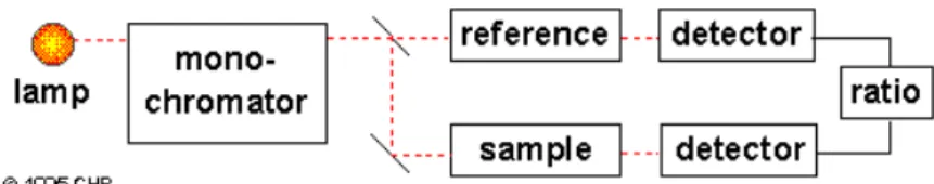
Figure 6. Schematic of a dual-beam UV-Visible spectrophotometer (CHP, 1995). ... 13

Figure 7. UV-Vis spectra at different nitrates concentrations (Thomas and Burguers, 2007). ... 14

Figure 8. Electromagnetic spectrum showing the NIR region (Wang 2003). ... 15

Figure 9. Flowsheet diagram of the experimental procedure. ... 20

Figure 10. N-NO3- behavior over time for (a) acetate, (b) propionate, (c) glucose, and (d) sucrose batch assays... 23

Figure 11. Carbon source behavior over time for (a) acetate, (b) propionate, (c) glucose, and (d) sucrose batch assays. ... 23

Figure 12. Spectra obtained for glucose throughout the batch assay VSS/COD=0.1 (a) UV-Visible and (b) NIR, and spectra obtained for acetate throughout the batch assay VSS/COD=0.1 (c) UV-Visible, and (d) NIR. ... 25

Figure 13. UV-Vis Spectra from each carbon source for the VSS/COD ratio of 0.1 (a) Acetate, (b) Propionate, (c) Glucose, and (d) Sucrose. ... 26

Figure 14. Pre-treatment of UV-Visible spectra (a) Acetate, (b) Propionate, (c) Glucose, and (d) Sucrose. ... 27

Figure 15. NIR Spectra from each carbon source for the VSS/COD of 0.1 (a) Acetate, (b) Propionate, (c) Glucose, and (d) Sucrose. ... 28

Figure 16. Pre-treatment of NIR spectra for all VSS/COD ratios studied (a) Acetate, (b) Propionate, (c) Glucose, and (d) Sucrose. ... 29

Figure 17. EMSPE related with LV for propionate batch assays (a) with the overall spectra, (b) with spectra range of 900-2000 nm. ... 30

Figure 18. (a) EMSPE related with LV, (b) N-NO3- measured and N-NO3- predicted by the PLS model for glucose batch assays in both cases. ... 30

L

T

Table 1. Wastewater composition allowed by Urban Waste Water Treatment European Directive.

Table 2. Specific carbon consumption rates obtained for all the batch assays. Table 3. Specific N-NO3- consumption rates obtained for all the batch assays.

Table 4. Spectroscopy-based (UV-Visible) N-NO3- PLS modeling results.

Table 5. Spectroscopy-based (UV-Visible) carbon sources PLS modeling results. Table 6. Spectroscopy-based (NIR) N-NO3- PLS modeling results.

Table 7. Spectroscopy-based (NIR) carbon sources PLS modeling results.

L

S

A

µ Reduced mass of the bonding atoms. BOD Biochemical Oxygen Demand c Speed light

COD Chemical Oxygen Demand E Photon energy

EMR Electromagnetic Radiation h Plank constant

k Forces constant

MLE modified ludzack ettinger MSC Multiplicative Scatter Correction N2 Nitrogen

N-NH4+ Ammonia

NIR Near infrared N-NO2- Nitrites

N-NO3- Nitrates

PCA Principal Component Analysis PLS Partial Least Squares

S Sugar

SG Savitzky-Golay filter SNV Standard Normal Variate TOD Total Organic Carbon UV Ultraviolet

ʋ frequency

VFA Volatile fatty acids VSS Volatile Suspend Solids y anharmonicity factor

λ Wavelenght

1.

I

1.1.

C

M

Depending on the origin of wastewater, different types of treatment can be applied. Therefore, the need to monitor wastewater and treatment processes arises to ensure a good quality of the treated effluent. Commonly, several compounds are need to be reduced such is the case of nitrates (NO3-).

The appearance of wastewater treatment processes (WWTP) to solve water quality issues led to the development of activated sludge processes, as a significant biological process in wastewater treatment plants which could be adapted to perform the removal of nitrogen and phosphorus.

Traditionally, parameters from WWTP are performed using analytical methods which are time consuming, and difficult to adapt to real time control. Thus, there is a clear need to search for novel techniques or improved tools.

Spectroscopy techniques have gain significant relevance in the past 30 years. With spectroscopy, transmission, absorption or vibrational properties of chemical species are measured in order to determine the concentration or identity of a sample. Once implemented and optimized, these methods are fast, non-destructive and user friendly allowing rapid inference of the process state.

UV-Visible spectroscopy has already proved to be an adequate technique for application in WWTP monitoring and it can be suitable for control purposes. However, it has some drawbacks associated to the limitation in the detection of some compounds. NIR spectroscopy is not so usually applied in WWTP monitoring. This technique has several advantages related to the detection of chemical and physical properties. However, more research is necessary for a better understanding of its applications and advantages when compared to standard methods.

The large amount of data in WWTP mainly operational analytical and physical data, and spectra analysis, requests the use of mathematical and statistical methods. The quantitative description of experimental results and effects extracting essential information in wastewater treatment has been performed using chemometric techniques. For instance, principal component analysis (PCA) is a common technique for finding patterns in data of high dimension, highlighting their similarities and differences. Partial Least Squares (PLS) is useful to predict a set of dependent variables from a large set of variables.

1.2.

O

The application of UV-Visible and Near-infrared (NIR) spectroscopy to monitor effluents could be an alternative method to standard analytical procedures. This report intended to use those techniques to evaluate denitrifying processes. Combining UV-Visible and NIR spectra with chemometric tools (multivariate analysis) aims to estimate models for different process parameters: Nitrate (NO3-),

and different carbon sources, such as: acetate, propionate, glucose, and sucrose. Different batch assays were performed with the following purpose:

• _{Establish the carbon source which gives the highest denitrifying results;} • _{Establish the best VSS/COD ratio to obtain higher denitrification rate;}

• _{Using spectral data to find a relationship between NO}3- concentration

measured and predicted by PLS models;

• _{Using spectral data to find a relationship between each carbon source} measured and predicted by PLS models.

1.3.

Wastewaters contain a large number of contaminants that needs to be eliminated or reduced. Actually, there are two well-known processes in wastewater treatment: physical and biological processes. The combination of both constitutes the primary, secondary and tertiary treatment. In the primary treatment, physical operations such as sedimentation processes are commonly performed to eliminate the settling solids presented in wastewaters. In the secondary treatment, biological and chemical processes are combined to eliminate most organic matter. The tertiary treatment is based on the combination of different processes and operations to eliminate components like nitrogen or phosphorus (Metcalf and Eddy, 2003).

The number of industries that flow wastewaters to domestic sewerage system has increased markedly in the last 20-30 years. It has been repeated the practice of combining industrial with domestic flow. A high number of wastewater treatment processes (WWTP) are finding alternatives to treat both flows separately, and are demanding a more advanced treatment of wastewater before the released to domestic wastewater collectors. The final treated wastewater stream to be discharged into natural environments must follow the Urban Wastewater Treatment European Directive (Table 1) that concerns the collection, treatment and discharge values of urban wastewater.

Table 1. Wastewater composition allowed by Urban Waste Water Treatment European Directive.

Contaminants Concentration (kg/m3₎

Total solids (TS) 0.035 Biological oxygen demand (BOD) 0.025 Total organic carbon (TOC) 0.035 Chemical oxygen demand (COD) 0.125 Total Nitrogen 0.010 Nitrites (N-NO2-) 0.010

Nitrates (N-NO3-) 0

Organic nitrogen 0

Free ammonia 0

Total phosphorus 0

Phosphates 0

Organic phosphorus 0 Inorganic phosphorus 0

Currently, most unit operations and processes used in wastewater treatment are being explored continuously and new operations and treatment processes are being developed with the objective of obtaining concentrations accomplishing the values permitted by legislation.

1.4.

B

N

R

Nitrogen removal is required to prevent eutrophication, for ground wastewater recharge or other applications. It can be either an integral part of the biological treatment system or an add-on process to an existing treatment plant. In WWTP a typical installation for biological elimination of nitrogen consists in two series tanks (Figure 1). The first tank is pre-anoxic (anoxic zone) and the second is oxic (aerobic zone). The amount of nitrogen eliminated depends on magnitude of recirculation that in general, is very high (Metcalf and Eddy, 2003).

Figure 1. Example of a biological nitrogen removal system (Metcalf and Eddy, 2003).

In the aerobic zone nitrification is obtained where ammonia (N-NH4+) is oxidized to

nitrate (N-NO3-). Afterwards, in the anoxic zone denitrification is performed where

N-NO3- and nitrites (N-NO2-) are reduced to nitrogen (N) (Metcalf and Eddy, 2003).

The denitrification process is the scope of the present work, thus, a detailed analysis to this biological process is performed in the next topic.

1.5.

D

The term denitrification was born in France in 1886 to describe the use of N-NO3- by

some bacteria to degrade substrate. The bacterial population uses N-NO3- and

N-NO2- to degrade substrate (Gerardi, 2002). Although denitrification is often

combined with aerobic nitrification to remove many forms of nitrogen compounds from wastewaters, the process occurs whenever an anoxic condition occurs. Denitrification removes nitrogen from the wastewater converting it to insoluble gases. Besides molecular nitrogen, nitrous oxide (N2O) is also produced during

denitrification from N-NO2- and N-NO3-. Although several groups of organisms are

capable of denitrification, including fungi and protozoa, most denitrifying organisms are facultative anaerobic bacteria.

In the following equations denitrification process is presented (Metcalf and Eddy, 2003).

6NO3- +2 CH3OH 6NO2- + 2CO2 + 4H2O (1)

6NO2-+3CH3OH 3N2 +3CO2+3H2O + 6OH- (2)

6NO2-+5CH3OH 5CO2 + 3N2 + 7H2O + 6OH- (3)

3NO3- + 14CH3OH +CO2+3H+ 3C5H7O2N+H2O (4)

1.6.

Q

N

There are relatively easy procedures to determine nitrogen forms in water. However, some of them are costly and require reagents addition. Among all usual parameters for water quality control, nitrogen is probably the most known and monitored particularly, N-NO3-. As it was previously reported, nitrogen is present in

water in reduced forms (organic and N-NH4+) and oxidized forms (N-NO2- and

N-NO3-). The presence of those different nitrogen compounds depends on

physic-chemical and biological mechanisms along the treatment process. Determination of N-NO3- is too the most important and more advanced investigation of compounds in

wastewater monitoring. UV-Vis spectroscopy is nowadays commonly used to detect and quantify N-NO3- concentrations in the wavelength range of 200-400nm (Paulo,

2008).

1.7.

UV-V

S

Electromagnetic radiation (EMR) interacts with atoms and produces characteristics absorptions and an emission profile (Figure 2). The principal parameter in EMR is the wavelength (λ) that is the distance between two peaks (Tomas and Burgers, 2007).

Figure 2. Sine wave representation of EMR (Tomas and Burgers, 2007).

The wavelength can be represented in function of frequency (ν), and knowing the fixed value of speed light (c):

𝜈 =𝑐_𝜆 (5) EMR behaves like a wave and particle, and the wavelength of such a particle, a photon, is related to energy of the photon by the equation:

𝐸 =ℎ𝑐_𝜆 109 ₍₆₎

where h is constant of Plank and E is energy of photon.

There is an enormous span of energies, over 18 orders of magnitude. Region of EMR can be seeing in Figure 3.

Figure 3. The electromagnetic spectrum (Tomas and Burgers, 2007).

When a photon interacts with an electron, they do not do this randomly but in a specific way. This interaction causes that electron obtain energy and it promotes to other exited state. It is obvious that on each state electron has different energy, and assuming a value of E (that is photon energy). It can be calculated by equation 6, with difference between states E2-E1 (E1 is ground state), the wavelength in which

excitation succeed.

With this, it can be seen that the wavelength of each absorption, depends on the difference between the energy levels. Each transition needs different amount of energy. It is expected that spectra has the form presented in Figure 4.

Figure 4. Idealised energy transitions for a diatomic molecule (Tomas and Burgers, 2007).

The intensity of absorption is linked to the type of transition and with a probability of that transition occurs. The part of the molecule that is involved in that transition is named chromophore. The spectrum that is the result of all chromospheres is the fingerprint that helps to identify specific molecules.

UV-Visible spectroscopic techniques used for quantifying purposes are based on Beer-Lambert law. According to the Beer-Lambert law for a single wavelength and a

single component, the following relation is valid (Paulo, 2008): 𝐴𝜆=𝜀𝜆𝑏𝑐 (7)

Where A – Absorbance (A.U.); ε - Molar absorptivity (mol-1_.cm-1_{); b - Path length of}

the cell in which the sample is contained (cm); c - Concentration of the absorber (mol.dm-3_).

To use equation 7 it must be assumed that: the radiation is monochromatic; the incidence of radiation beam is normal; the temperature is constant; no molecular

interactions between the absorber and the other molecules; and there are no uncompensated losses (Burgess, 2007; Paulo, 2008).

1.7.1.

I

Single-Beam spectrophotometers are often sufficient for making quantitative absorption measurements in the UV-Vis spectral region. The concentration of an analyte in solution can be determined by measuring the absorbance at a single wavelength. Those spectrophotometers can use a fixed wavelength light source or a continuous source. The simplest instruments use a single-wavelength light source, such as a light-emitting diode (LED), a sample container, and a photodiode detector. In either type of single-beam instrument, the instrument is calibrated with a

reference cell containing only solvent

to determine the (Po) (initial

power of the light) value necessary for

an absorbance measurement

(Blanco and Villarolla, 2002).

Figure 5. Schematic of a wavelength-selectable, single-beam UV-Visible spectrophotometer (B.M. Tissue, 2001).

The double-beam spectrophotometers greatly simplify the process by measuring the transmittance of the sample and solvent simultaneously. The detection electronics can then manipulate the measurements to give the absorbance. The dual-beam design simultaneously measure P and Po of the sample and reference cells,

respectively. Most spectrometers use a mirrored rotating chopper wheel to alternately direct the light beam through the sample and reference cells. The detection electronics or software program can then manipulate the P and Po values as the wavelength scans to produce the spectrum of absorbance or transmittance as a function of wavelength (Thomas and Burgers, 2007).

Figure 6. Schematic of a dual-beam UV-Visible spectrophotometer (CHP, 1995).

1.7.2.

A

With spectrophotometry, can be measured the unknown concentration of a sample. First, the choice of the absorption band needs to be accomplished. If this procedure is not possible, double-beam spectrophotometry has to be performed to know where its absorption band will lie (Perkampus et al., 1992).

Generally, all the organic compounds will absorb in the UV-visible range of the spectrum and so a number of biological compounds may be measured using UV-visible spectrophotometer (Perkampus et al., 1992).

In the case of UV absorption, NO3- is rather sensitive with a half Gaussian shape for

low concentrations (between 0.5 and 15 mg NO3-/L for 10 mm path length). When

NO3- concentration increases, an absorption peak appears around 310 nm from 0.2 g

NO3-/L, for 10 mm path length. This typical response is exploited for NO3-

determination with different wavelength ranges in function of the expected concentration. Actually, two forms of NO3- ions exist in relatively concentrated

solutions (around 5 g/L); with a very slight difference in their UV spectra (Thomas and Burgers, 2007).

Figure 7. UV-Vis spectra at different nitrates concentrations (Thomas and Burguers, 2007).

A large number of studies have been conducted for NO3- determination using

spectral data. Those are classified in three groups, according to method used (Thomas and Burguers, 2007):

• _{I: It is used one absorbance with values between 205 and 220 nm and other} absorbance used like a compensatory with absorbance between 250 and 275 nm;

• _{II: It is used a second derivative with estimation of a three wavelengths} between 220 and 225 nm. This method is less sensitive and assumes constant interferences;

• _{III: A PLS algorithm is used with a range between 220 and 350 nm. This is} considered the most efficient and fast method.

1.8.

N

-I

(NIR)

S

Infrared is the electromagnetic energy of molecular vibration. The energy band is defined by three groups: Near-Infrared (780-2500nm), Infrared (or mid-infrared) (2500-25000nm), and far infrared (25000-1000000nm).

The molecules vibration can be described using the harmonic oscillator model, by which the energy of the different, equally spaced levels can be calculated from the following equation:

𝐸𝑣𝑖𝑏 =�ʋ+1₂�_2𝜋ℎ �𝑘_µ (8)

where ʋ is the vibrational quantum number, h the Planck constant, k the force constant and µ the reduced mass of the bonding atoms (Blanco and Villaroya, 2002). Only those transitions between consecutive energy levels (∆ʋ=±1) that causes a change in dipole moment are possible:

∆𝐸𝑣𝑖𝑏 =∆𝐸𝑟𝑎𝑑=ℎʋ (9)

The harmonic oscillator model cannot explain the behavior of actual molecules, as it does not take account of Columbic repulsion between atoms or dissociation of bonds. As a result, the behavior of molecules more closely resembles the model of a harmonic oscillator, by which energy levels are not equally spaced. Thus, energy difference decreases with increasing ʋ:

∆𝐸𝑣𝑖𝑏=ℎʋ1−2ʋ+∆ʋ+ 1𝑦 (10)

Where y is the anharmonicity factor (Blanco and Villaroya, 2002). The spectral range interfaces the visible and infrared portions of the

electromagnetic spectrum and there is a big controversy related to the definition of its limits (Figure 8).

Figure 8. Electromagnetic spectrum showing the NIR region (Wang 2003).

1.8.1.

I

Spectrophotometers have a detector and a dispersive (a diffraction grating) to obtain the different wavelengths. Fourier transform NIR instruments using an interferometer are also common, especially for wavelengths above 1000 nm. The spectrum can be measured as much reflection as transmission (depending on the

sample). Common incandescent or quartz halogen light bulbs are often used as broadband sources of NIR radiation for analytical applications. Light-emitting diodes (LEDs) are also used, offering greater lifetime and spectral stability and reduced power requirements. The detector is selected in function of range of wavelengths that are measured (Blanco and Villarolla, 2002).

1.8.2.

NIR

Many materials show their properties only in the NIR spectral region. The absorption, fluorescence, photosensitizing, photoconductive, photochromic, and other properties in the NIR spectral region are all being explored for various applications in many sectors. For example, NIR dyes are used as contrast-enhancing agents for spectroscopic optical coherence tomography and as an NIR photosensitizer in photodynamic therapy for alternative treatment for cancer and several other medical conditions (Wang, 2013).

1.9.

C

The term “chemometrics” has more than 40 years. It was born with the purpose to describe the techniques and operations associated with mathematical manipulation and interpretation of chemical data. Modern instrumentation laboratory has a really high amount of graphical and numerical data. The identification and interpretation of the data that instrumentation shows can be limited by error and can limit an effective operation of the laboratory. Increasingly, sophisticated analytical instrumentation is also being employed out of the laboratory, for direct on-line or in-line process monitoring. Chemometrics is a complementary tool to laboratory automation. Thus, chemometrics seeks to apply mathematical and statistical operations to aid data handling (Adams, 1995).

The appearance of chemometrics gave a new motivation to the use of spectroscopy techniques in quantitative and qualitative applications. The usefulness of chemometric tools lies in the possibility to extract information in a very efficient spectrum, allowing relating the spectral patterns with varying chemical and physical properties of the samples. In addition, regarding the difficulty of physical interpretation of a spectrum, the application of empirical mathematical tools has been suggested. Therefore, principal component analysis (PCA) to unravel spectral patterns and partial least squares (PLS) for regression models have been recently used.

1.10.

P

-

Each spectrum contains a large amount of information related with both physical and chemical levels. The extraction of this information requires the application of pre-processing and spectral processing. The pre-processing is commonly used by applying corrective methods caused by interferences and deficiencies in the acquisition of each spectrum. Light scattering is one of the main problems when it is intended to evaluate a chemical composition of a sample. Thus, it is imperative to apply corrective methods to eliminate those interferences. In the topics presented below the most common pre-processing types used in spectroscopy are described.

1.10.1.SAVITZKY AND GOLAY FILTER

Savitzky-Golay (SG) is a technique that has the name of their authors. This technique has become a classic in analytical signal processing and least-squares polynomial smoothing is probably the technique widespread used in spectral data processing and manipulation. This technique is commonly used as a pre-treatment to remove interferences and noises in spectral data from different type of samples. The filter is used as a sequence of three steps. In the first step the filter order is defined. Afterwards, the filter dimension is also defined. The third step comprises the selection of coefficients according to the table described in Páscoa (2006) and divided by a constant which depends on the dimension filter obtained in the second step.

1.10.2.MEAN-CENTERING

The mean-centering data-preprocessing option is performed by calculating the average data vector or a spectrum of all rows in a data set and subtracting it point by point from each vector in the dataset. It is slightly inconvenient to use when processing chromatographic-spectroscopic data since the origin of the model is changed (Gemperline, 2006). It is advisable to use mean-centering under many circumstances prior to PCA analysis. To use mean centering, it is necessary to substitute the mean-centered data matrix AT _{into the singular-value decomposition}

and in all subsequent calculations where A is combined with the U, S, or V from the principal component model.

𝑎𝑖𝑗𝑇 =𝑎𝑖𝑗−_𝑛1∑𝑛𝑖=1𝑎𝑖𝑗 (11)

Where𝑎𝑖𝑗𝑇 is the mean of the spectra, 𝑎𝑖𝑗 is the spectra in one point, and n is the

number of spectra.

The new model based on AT _{can be transformed back to the original matrix, A, by}

simply adding the mean back into the model as shown in the following equation:

𝐴 − 𝐴̅=𝐴𝑇 _{=𝑈𝑆𝑉}𝑇 ₍₁₂₎

Where A is the original matrix of spectra,𝐴̅ is the mean matrix, 𝐴𝑇 _is

mean-centered data matrix. The product US represents the n × d matrix of principal component scores, V denotes the m × d matrix. Mean-centering changes the number of degrees of freedom in a principal component model from k to k + 1.

1.10.3.STANDARD NORMAL VARIATE

Standard Normal Variate (SNV) previously described by Barnes et al. (1989), centers and scales individual spectra, having an effect very much like that of Multiplicative Scatter Correction (MSC).

Equation (13) shows how SNV is applied:

𝑥�𝑖𝑘 =𝑥𝑖𝑘_𝑠−𝑚_𝑖 𝑖 (13)

where xik is the spectral measurement, mi is the mean of the k spectral measurements for sample i and si is the standard deviation of the same K measurements.

This kind of pre-treatment is used in many spectroscopic applications. It is performed without a reference spectrum, improving predicting precision but not simplifying the model. SNV standardizes each spectrum using only the data from that spectrum and not using the mean spectrum of any set (Paulo, 2008).

1.11.

P

L

S

R

Partial least squares (PLS) is a major regression technique for multivariate data. PLS has been applied to many fields in science with great success. One important feature of PLS is that it takes into account errors in both the concentration estimations and spectra.

Two sets of models are obtained as follows:

X = TP + E, c = Tq + f (14)

where, the T matrix contains the scores of I objects on K principal components. The P matrix is a square matrix and contains the loadings of J variables on the K principal components. E is the error matrix. Q, has analogies with a loadings vector, although is not normalized. In the first equation, the product of T and P approximates to the spectral dataset obtained through the experimental work and in the second equation product of T and q approximates the concentration estimation (Carvalho et al., 2005).

It is important to determine how many significant PLS components are necessary using cross-validation (CV). The basis of the method consists in the prediction ability of a model created with one part of a dataset. Subsequently, the model is normally tested by how well it predicts the remained dataset. CV is employed as a method for determining how many components are able to characterize the data. This technique has been successfully applied by Sarraguça et al. (2009), Blanco and Villaroya (2002), Al-Mbaideen and Benaissa (2011).

The estimated mean squares prediction error (EMSPE), or its square root, is frequently used to assess the performance of regressions. It is also used for choosing the optimal number of components (latent variables – LV) in PLS (Mevik and Cederkvist, 2005).

EMSPE measures the expected squared distance between what your predictor predicts for a specific value and what the true value is.

𝐸𝑀𝑆𝑃𝐸=𝐸�∑𝑁𝑖=!(𝑔(𝑥𝑖)− 𝑔�(𝑥𝑖))2� (15)

in which N denotes the number of observations, g(xi) is the given value of the analyte of interest and g(xi) is the value predicted by the PLS. Given a certain data set, the EMSPE values are calculated for different numbers of components included in the PLS. Normally the EMSPE reduces with increasing number of PLS components until a minimum or constant value is reached and the corresponding number of components is regarded as optimal (Akbulut, 2014).

2.

M

2.1.

S

I

Suspended sludge from an activated sludge tank and obtained from a municipal wastewater treatment plant, was used as seed sludge for starting the experiments under mesophilic conditions.

2.2.

S

M

C

Four carbon sources, two volatile fatty acids (VFAs) (acetate and propionate) and two sugars (glucose and sucrose) were used separately and KNO3 was used as the

nitrate source with a constant ratio between carbon and nitrogen (C/N). A constant C/N was set to get insights about denitrifying conditions. The medium has been described in Cortez et al. (2009) and contained the following composition (per L): 93 mg K2HPO4, 18 mg KH2PO4, 24.2 mg CaCl2·2H2O and 409.2 mg MgSO4·7H2O and

100 mL of trace metals (next described). Due to the medium buffering capacity, no pH adjustment was performed.

The trace metals solution has been described in Smolders et al. (1994) and consisted of (per L): 1.5 g FeCl3·6H2O, 0.15 g H3BO3, 0.03 g CuSO4·5H2O, 0.18 g KI, 0.12 g

MnCl2·4H2O, 0.06 g Na2MoO4·2H2O, 0.12 g ZnSO4·7H2O, 0.15 g CoCl2·6H2O.

Before inoculation, each medium was distributed into serum bottles, sealed with butyl rubber septa and aluminum crimp caps, and flushed with N2 to guarantee

anoxic conditions.

2.3.

V

S

S

(VSS)

The VSS were determined according to methods 2540 D and 2540 E from Standard Methods (APHA, 1999). Glass-fiber filter disks were washed in a filtration apparatus with distilled water. The filter disks were transferred to an aluminum weighting dish and ignited at 550°_{C during 30 min in a muffle furnace. The disk and aluminum}

dish were cooled in a desiccator and then weighted (m1). A homogeneous sample in

triplicate was used (V = 5 mL). These samples were filtered in a filtration apparatus and the glass-fiber disk, aluminum dish and residue retained on the filter (set) were dried at 105°C during one day. After, the set was cooled in a desiccator and then weighed (m2). Afterwards, VSS were determined where the residue from later

procedure was ignited at 550°C in a muffle furnace during 2 hours (m3), and the

following equation was used:

𝑉𝑆𝑆 (𝑔_𝐿) =(𝑚2−𝑚3_𝑉 )× 1000 (16)

2.4.

E

S

To get a suitable consortium, the fresh biomass was first acclimatized (Lee and Col, 1995) in four denitrifying synthetic mediums, in anoxic conditions, at 30°C. According to Dhamole et al. (2006), sludge acclimatization is a necessary process to allow the development of an efficient consortium to treat high nitrate loads. Thus, in the present work the acclimatization process was performed. Regarding the findings of Cortez et al. (2009), the use of C/N = 1.5 is advantageous to denitrification, thus, this ratio was selected throughout this work.

The experimental setup is schematically represented in Figure 9 where after the sludge acclimation to each synthetic medium, new batch assays were conducted with four selected VSS/COD ratios in order to select the highest carbon and nitrate removal rates. It is important to notice that after acclimation period to each carbon source, the growing conditions might be different (Muyo 2007), thus, VSS were again measured to prepare new batch assays with different VSS/COD ratios. The

assays were performed in triplicate, however, since it was not possible to guarantee the exactly same amount of inoculum no average values were determined.

Figure 9. Flowsheet diagram of the experimental procedure.

For each experiment, samples were taken using syringes and needles over time. Samples were centrifuged at 10000 rpm for 10 minutes, and the supernatant was filtered and stored for the analytical measurements and for spectroscopy analysis.

2.5.

N

(NO

)

This method is used for samples with a low concentration of organic matter, non-natural waters and contaminated drinking water based on UV spectrophotometry. Organic matter, carbonates, bicarbonates, nitrites, and hexavalent chromium interfere with the method. Interference nitrites, carbonates and bicarbonates can be eliminated by adding sulfamic acid to the sample. This compound promotes the reduction of nitrite ion to N2. The organic matter, absorbs at 220 nm, interfering

with NO3-. As the NO3- does not absorb at 275 nm, a second measurement made at

this wavelength can be used to correct the interference at 220 nm.

Two solutions were prepared with deionized water: sulfamic acid (0.05M) and a stock solution of nitrate (100 mg/L N-NO3-). Afterwards a nitrate work solution was

prepared diluted from the stock solution (50mg/L N-NO3-).

Samples were diluted with sulfamic acid using the same proportion (Thomas and Burgers, 2007) and analyzed reading the absorbance at 200 nm and 275 nm using a spectrophotometer UV-Visible (JASCO V560). A calibration curve was used to calculate the final N-NO3 concentrations.

2.6.

V

F

A

(VFA

)

S

VFAs were determined by high-performance liquid chromatography (HPLC) (JASCO, Tokyo, Japan) with automatic injection, using a UV detector (210 nm). The column used was a Varian (Palo Alto, CAUSA) Metacarb 67H operating at a temperature of

60 °C. The eluent was a solution of sulfuric acid (0.005 mol/L) with a flow rate of 0.60 mL/min and a pressure of between 60–70 kg/cm2_.

Sugars were also determined by HPLC (JASCO, Tokyo, Japan) with automatic injection, using an IR detector. The column used was a Varian (Palo Alto) Metacarb 87H. The eluent was a solution of sulfuric acid (0.005 mol/L). The conditions were modified depending on the sugar to be analyzed. For glucose, the column operated at a temperature of 60 °C. A flow rate of 0.70 mL/min and a pressure of between 60– 80 kg/cm2 _{was used. For sucrose, the column operated at a temperature of 35 °C. A}

flow rate of 0.30 mL/min and a pressure of between 30–40 kg/cm2 _{was used.}

For all the HPLC analysis, internal standards were used and the integration of all peaks was performed using the software for the HPLC (Varian Star Workstation). Calibration curves were also performed to measure the final concentrations.

2.7.

S

C

R

Specific substrate consumption rates of nitrate and each carbon source were determined according to the following equation (Cortez et al., 2009):

𝑑𝑆= _𝑉𝑆𝑆𝑆0−𝑆𝑡 _×𝑡 (17) where dS is the specific substrate consumption rate, S0 and St are the substrate

concentrations at the beginning and at the end of the batch test, respectively, and VSS is the concentration of volatile suspended solids during the denitrification batch test time t.

2.8.

UV-V

N

-I

(NIR)

S

Samples taken over time and from each experiment were analyzed in a UV-visible spectrometer (JASCO V560) using a quartz cell with a path length of 1 cm, and in a NIR spectrometer (ABB).

2.9.

C

T

The software Matlab™ 8.1 (The Mathworks, Natick, MA) was used for UV-Visible and NIR spectral data pre-treatment and for predicting acetate, propionate, glucose, sucrose and N-NO3- by PLS models with a total of 60 observations for each batch

assay. A cross-validation (CV) was performed and the latent values (LV) were selected based on the Estimating Mean Squares Prediction Error (EMSPE). Also the correlation coefficients (R2) were obtained for the spectroscopy techniques applied.

3.

R

The main purpose of this work was to find alternative techniques (UV-Visible and NIR spectroscopy) to characterize wastewaters surpassing the need of analytical procedures which have been shown as time-consuming methods.

First, results provided by the analytical methods are presented and discussed regarding denitrifying conditions taking into account the removal of nitrate and each carbon source, and specific consumption rates. Three experiments were

performed for each carbon source and VSS/COD ratio, however, for a more clear discussion only one example will be further used.

Afterwards, an in-depth analysis is given to UV-Visible and NIR spectroscopy considering each batch assay. A PLS analysis is also performed combining the analytical measurements and all the spectra collected.

3.1.

D

Recently, microbial ecology involved in denitrification in wastewater treatment has been investigated for an enhancement of process performance. The majority of these bacteria have been found as nitrate reducers, followed by the denitrifiers, while the most prevalent truncated denitrifiers reported are those deficient in nitrate reductase (Teixeira et al., 2010). For this reason a consortium of appropriate and efficient microorganisms would remove nitrate from the wastewater more efficiently (Zala et al., 1999). In this way, the use of activated sludge as a consortium of denitrifying bacteria can be extremely advantageous.

In wastewater treatment most denitrifying bacteria are heterotrophic, thus an organic carbon source is required. Acetate has been reported to give high denitrification rates in most cases (Mohseni-Bandpi et al., 1999; Sanches et al., 2000; Hallin et al., 2006). Besides the type of carbon source, denitrification rate is strongly susceptible to the concentration of the carbon source and the C/N (Gálvez et al., 2003; van Rijn et al., 2006). Figure 11 shows the behavior of N-NO3- over time for

the experiments performed with each carbon source added and after the acclimation period.

It is important to notice again the required prior VSS determination before each experiment to quantify the COD depending on the VSS/COD ratio. Consequently, the concentration of each carbon source as well as N-NO3- is different keeping the C/N

ratio constant (1.5).

As an overall analysis, it can be seen from Figure 11 that NO3- was removed from the

wastewater throughout the experimental period. However, differences between VFAs and Sugars are quite clear, indicating that the biomass has more affinity to VFAs rather than sugars. It was found that for acetate N-NO3- removal percentages

were higher than 80%, and for propionate, more than 90% of N-NO3- was removed

from the effluent. Regarding the experiments provided with glucose, also lower removal percentages of N-NO3-. 69% was attained for the experiment with

VSS/COD=0.1, 65% for VSS/COD=0.3, 58% for VSS/COD=0.5, and 60% for VSS/COD=1. Lower removal percentages of 31% (VSS/COD=0.1), 21% (VSS/COD=0.3), 35% (VSS/COD=0.5), and 6% (VSS/COD=1) were achieved for the experiment with sucrose (Figure 10d).

Figure 2. N-NO3- behavior over time for (a) acetate, (b) propionate, (c) glucose, and (d) sucrose batch

assays.

Figure 3. Carbon source behavior over time for (a) acetate, (b) propionate, (c) glucose, and (d) sucrose batch assays.

Figure 11 shows the behavior of acetate, propionate, glucose, and sucrose over time for the experiments performed with each carbon source added and after the acclimation period.

It can be seen from Figure 12 that acetate, propionate, glucose, and sucrose were removed from the wastewater throughout the experimental period. However, differences between VFAs and Sugars are again detected taking into account the biodegradability of the effluent. It was found that acetate removal percentages were higher than 87% and propionate removal percentages were higher than 94%. The experiments with sugars presented for glucose, removal percentages higher than 71%, and lower than 78% for sucrose.

3.2.

S

The microbial activity is considered a key parameter in wastewater treatment and is commonly expressed in terms of substrate removal ability. The determination of the denitrifying microbial activity was performed for all the batch assays and was expressed as specific consumption rates for nitrate and for each carbon source (Tables 2 and 3).

Table 8. Specific carbon consumption rates obtained for all the batch assays.

VSS/COD Specific carbon consumption rate (g carbon source g-1 _{VSS h}-1₎

Acetate Propionate Glucose Sucrose

0.1 2.10 1.72 1.20 0.58

0.3 0.86 0.65 0.60 0.29

0.5 0.50 0.42 0.29 0.08

1 0.25 0.20 0.02 0.27

Table 9. Specific N-NO3- consumption rates obtained for all the batch assays.

VSS/COD Specific N-NO3- consumption rate (g N-NO3- g-1 VSS h-1)

Acetate Propionate Glucose Sucrose

0.1 0.52 0.45 0.27 0.28

0.3 0.13 0.07 0.12 0.24

0.5 0.13 0.06 0.06 0.14

1 0.13 0.06 0.06 0.03

It can be seen from Table 2 that the batch assays performed with VFAs presented specific carbon consumption rates higher than the ones performed with sugars. Using acetate as the sole carbon source a better biomass activity was found when compared with propionate batch assays, even though an acceptable result was also achieved with this carbon source. Comparing the four VSS/COD ratios studied, 0.1 and 0.3 provided the best results, even with sugars. It was already stated by Muyo (2001) that the carbon removal increases using a VSS/COD ratio between 0.1 and 0.3. Since VSS/COD ratios are dependent on the VSS concentration, lower ratios indicate that a higher carbon concentration is added.

Regarding Table 3, higher specific N-NO3- consumption rates were attained for VFAs,

and again, the best VSS/COD ratios are 0.1 and 0.3. This could be again related with the determination of COD (carbon source concentration) and consequently the N-NO3- concentration needed to provide a constant C/N ratio. Thus, if a high amount of

carbon is added also a high amount of N-NO3- is needed. According to Bilanovic et al.

(1999), Metcalf and Eddy (2003), Paul and Liu (2012), and Muyo (2001), the denitrification process also increases with VSS/COD ratios between 0.1 and 0.3, which is in agreement with the results presented in Table 3. When compared with the study of Muyo (2001) where a specific consumption rate of 0.006 g N-NO3- g-1

VSS h-1 _{was found using the same initial concentration of N-NO3-, a clear}

improvement of the denitrification process was achieved with the present work. Regarding the results obtained from Table 2 and Table 3, acetate was selected as the best carbon source and 0.1 was selected as the best VSS/COD ratio.

3.3.

V

A

UV-V

NIR

S

For each batch denitrifying assay, UV-Visible and NIR spectra were obtained over time. Since different types of sugars (e.g. glucose or sucrose)cannot be directly detected by UV-Visible spectroscopy it was found interesting to study if NIR spectroscopy could be more effective in the detection of these mediums (Paulo, 2008). VFAs are being reported as well detected using UV-Visible spectroscopy. Thus, a global analysis of each spectroscopy technique was first performed. Figure 12 shows UV-Visible and NIR spectra obtained for one batch assay of glucose and acetate with VSS/COD = 0.1.

Figure 4. Spectra obtained for glucose throughout the batch assay VSS/COD=0.1 (a) UV-Visible and (b) NIR, and spectra obtained for acetate throughout the batch assay VSS/COD=0.1 (c) UV-Visible, and (d) NIR.

In Figure 13 UV-Visible and NIR raw spectra of the batch assays for glucose and acetate are presented. By analyzing the different spectra is already possible to detect the main differences between the UV-Visible and the NIR spectra.

In the case of UV-Visible spectra, and regarding acetate batch assay, a variation in the composition can be visually detected by a change of the spectra’s shape, giving already some information, which could be related with NO3- and/or carbon source.

An expressive shift is observed for glucose batch assay in UV-Visible spectra only for one sample which corresponds to the medium without biomass activity. Looking to

the small window without that spectrum in Figure 13a, no clear differences between spectra data were found which is in agreement with the findings of Paulo (2008). In NIR spectra the changes are very difficult to be noticed with naked eye when VFAs are analyzed. A slight difference was observed in NIR spectra of glucose batch assay. The baseline shifts are suggested to be due to medium turbidity and its natural decrease along the dilutions, what could be detected by the visible part of the spectrum.

Next sections will present results regarding only UV-Visible spectra for a more clear analysis and discussion. Afterwards, an in depth analysis will be performed to NIR spectra.

3.4.

UV-V

S

A global analysis to UV-Visible spectra without pre-treatment for the batch assays considering all carbon sources was performed and is presented in Figure 13.

Figure 5. UV-Vis Spectra from each carbon source for the VSS/COD ratio of 0.1 (a) Acetate, (b) Propionate, (c) Glucose, and (d) Sucrose.

From Figure 13 it is clearly seen a difference between each carbon source. The variability between each spectrum could be possible due to the carbon source added or to the nitrate concentration. Also it is important to notice the possibility of some interferences if the samples are not well centrifuged of filtrated. This could be attributed to the variability in the baseline of propionate or glucose batch assays. A less variability was found for acetate and sucrose batch assays.

3.5.

UV-V

S

-

A pre-treatment method was applied to the entire UV-Visible spectra: standard normal variate (SNV) and mean-centering. In this case, the selection and optimization of smaller spectral ranges for the analysis was not desired since the main goal was to study the influence of pre-processing for all the acquired information and not only a part. Figure 14 shows all the spectra acquired for each carbon source with pre-treatment.

Figure 6. Pre-treatment of UV-Visible spectra (a) Acetate, (b) Propionate, (c) Glucose, and (d) Sucrose. The application of pre-treatment methods was able to show differences in the case of VFAs (acetate and propionate) (Figure 14). Regarding sugars (glucose and sucrose), pre-treatment methods seems do not reflect a difference between samples, corroborating the findings of Paulo (2008). It can be also seen that the highest variability is located in the wavelengths ranges between 200-250 nm and between 250-380 nm which are commonly related to NO3- concentrations variability

(Thomas and Burgers, 2007; Sarraguça et al., 2009). This will be further analyzed and discussed by chemometric techniques.

3.6.

NIR

S

-

A global analysis to NIR spectra without pre-treatment for the batch assays considering all carbon sources was performed and is presented in Figure 15. Afterwards, a pre-treatment method was applied to the entire NIR spectra: Savitzky-Golay (SG), standard normal variate (SNV) and mean-centering (MCN). Figure 16 shows the NIR spectra with pre-treatment for all the carbon sources batch assays.

From Figure 16, no clear differences were observed between each batch assay with the four carbon sources using the overall NIR spectra. Only a slight variability with propionate and glucose as sole carbon sources was obtained. This could be related to some difficulties regarding sample pre-treatment. Since the wavelength range in NIR is somewhat larger than UV-Visible, a selection of a minor wavelength range is always an important step prior to chemometric application.The pre-treatment NIR spectra presented in Figure 16 shows no visual perceptible differences, and again only the spectra related to glucose and propionate have a slight difference between

each sample.

Figure 7. NIR Spectra from each carbon source for the VSS/COD of 0.1 (a) Acetate, (b) Propionate, (c) Glucose, and (d) Sucrose.

Figure 8. Pre-treatment of NIR spectra for all VSS/COD ratios studied (a) Acetate, (b) Propionate, (c) Glucose, and (d) Sucrose.

3.7.

P

L

S

The PLS was used with the aim of correlating the spectra with each carbon source and with NO3- concentrations obtained throughout each batch assay. The spectra

and the values of effluent concentration were mean-centered. The number of LV was estimated by CV. The model minimum error (EMSPE) was first evaluated through the use of the overall UV-Visible and NIR spectra.Afterwards, the wavelength ranges where a highest variability is located were analyzed. For UV-Visible spectra the range was 200-350 nm and for NIR spectra the range was 900-2000 nm as it was already reported by Sarraguça et al. (2009). Figure 17 shows an example of the EMSPE obtained for the overall NIR spectra and for the selected NIR spectra range.

(a) (b)

(c) (d)

Figure 9. EMSPE related with LV for propionate batch assays (a) with the overall spectra, (b) with spectra range of 900-2000 nm.

The minimum EMSPE value is not well defined regarding Figure 17a. Considering only the spectra range selection (Figure 17b), the minimum EMSPE is well defined through giving the possibility to choose the number of LV. Thus, throughout the PLS models analysis this methodology was implemented.

An example is further presented in Figure 18 illustrating how the PLS model is obtained from NIR spectral data. First, the CV analysis for different numbers of LV was performed. Based on the minimum error of the model (EMSPE) the number of LV was chosen (Figure 19a). For all methods and parameters, the minimum EMSPE value is well defined, thus providing a good indication of the appropriate number of LV for each model. Subsequently, the PLS regression is obtained considering the measured and predicted values (Figure 19b).

Through CV analysis, 4 LV were chosen for the model (minimum error). The EMSPE obtained was 0.35 g/L (Figure 18a). It is noted in this case that there is a clear minimum in the curve. N-NO3- concentrations obtained by the reference method are

shown in Figure 19b as a function of values predicted by the PLS model with 4 LV. It is important to notice that a low error was obtained by the model (EMSPE = 0.35 g/L) and consequently the correlation coefficient (R2_{) was 0.89. It is possible to}

conclude that the equipment used is capable of monitor effluent N-NO3- even

considering a variation range of relatively short concentrations.

Figure 10. (a) EMSPE related with LV, (b) N-NO3- measured and N-NO3- predicted by the PLS model for

glucose batch assays in both cases.

The PLS analysis is presented in Table 4 using UV-Visible spectral data for the prediction of N-NO3- concentrations. Acetate, propionate, glucose, and sucrose

concentrations PLS results are presented in Table 5 considering all batch assays and UV-Visible spectral data.

Table 10. Spectroscopy-based (UV-Visible) N-NO3- PLS modeling results.

Prediction of N-NO3-

Acetate Propionate Glucose Sucrose

LV 5 3 2 2

EMSPE (g/L) 7 2.5 1 0.7 R2 _{0.29 0.20 0.12 0.90}

Table 11. Spectroscopy-based (UV-Visible) carbon sources PLS modeling results. Prediction of each carbon source Acetate Propionate Glucose Sucrose

LV 2 2 2 2

EMSPE (g/L) 50 28 30 3.2 R2 _0.21 a _{0.30 0.94}

a _{no coefficient correlation was found}

In the case of N-NO3-, the best correlation coefficient (R2) was obtained with sucrose.

The highest EMSPE were achieved for VFAs. In the case of acetate, the error is the maximum concentration added to the batch test. Glucose was not predicted by the PLS model due to the low range of concentrations.

The EMSPE obtained for the PLS models of each carbon sources were very high and consequently low correlation coefficients were obtained indicating that UV-Visible spectroscopy is not able to measure the studied carbon sources. However, in spite of the high EMSPE for sucrose, an acceptable correlation coefficient was found.

In Table 6 PLS results are presented using NIR spectral data for the prediction of N-NO3- concentrations. Acetate, propionate, glucose, and sucrose concentrations PLS

results are presented in Table 7 considering all batch assays and NIR spectral data.

Table 12. Spectroscopy-based (NIR) N-NO3- PLS modeling results.

Prediction of N-NO3-

Acetate Propionate Glucose Sucrose

LV 9 4 4 13

EMSPE (g/L) 2.3 0.07 0.35 1.1 R2 _{0.87 0.90 0.89 0.99}

Table 13. Spectroscopy-based (NIR) carbon sources PLS modeling results. Prediction of each carbon source Acetate Propionate Glucose Sucrose

LV 2 3 10 3

EMSPE (g/L) 49 29 3.1 2.7 R2 _{0.14 0.65 0.98 0.94}

Regarding the results obtained for NIR spectral data, low EMSPE were achieved for all batch assays and the PLS models had regression coefficients higher than 0.85 for the prediction of N-NO3- (Table 6). Even with the low range of concentrations, and

considering the high N-NO3- added to each batch test good prediction abilities were

obtained not quite distant from 1.

The best results obtained in the NIR range were those for glucose and sucrose (sugars), with a minimum error EMSPE of 3.1 g/L and 2.7 g/L, respectively. This result indicates the high sensitivity of NIR spectroscopy to sugar changes in the effluent composition. Quite the opposite results were the PLS models to predict VFAs. Very high EMSPE were obtained, indicating that NIR spectroscopy is not capable to predict VFAs as sole carbon sources.

The present work revealed that measuring N-NO3- concentrations is not suitable by

using UV-Vis spectroscopy. These results were found relatively diverged from the ones of Sarraguça et al. (2009). Regarding NIR spectroscopy, and when compared to Sarraguça et al. (2009), better prediction abilities were found using four different carbon sources. In the case of the different carbon sources studied, Sarraguça et al. (2009) only tested the prediction ability of COD and established that UV-Visible spectroscopy provided the best overall results. In the present case, sucrose concentration was fairly predicted using both spectroscopy techniques. VFAs were not satisfactorily predicted mainly due to the low concentration range obtained in each batch assay, decreasing data variability for PLS models application.

4.

G

C

Form this work it was found that nitrate was removed from all the batch assays as well as the four carbon sources used, indicating that denitrifying conditions were achieved. The biomass had more affinity to VFAs given the high removal efficiencies percentages (more than 80% for nitrate and carbon source).

Regarding specific consumption rates for both carbon sources and nitrates, it was possible to conclude that acetate was found as the best carbon source and 0.1 was selected as the best VSS/COD ratio.

Taking into account the pre-processing UV-Visible spectral data, experiments with sucrose provided the best N-NO3- prediction ability. It was also possible to conclude

that UV-Visible spectroscopy was not able to predict the carbon sources tested. NIR spectral data showed a fairly N-NO3- prediction ability even with a low range of

concentrations. Quite satisfactory results were obtained regarding sugars detection and prediction based on NIR spectroscopy.

This work demonstrates the usefulness of spectroscopy techniques for biological processes monitoring. As a suggestion, to define the best wavelength range, the study of other spectral ranges could be implemented in order to compare with the ones selected in the present work. Monitoring a continuous system with the same conditions tested in batch assays is also suggested.

R

Adams, M.J. 1995. Chemometrics in analytical spectroscopy. The Royal Society of Chemistry, (1995) United Kingdom.

Akbulut, S., Validation of classical quantitative fundamental parameters method using multivariate calibration procedures for trace element analysis in ED-XRF, J. Anal. At. Spectrom. (2014) in press.

Al-Mbaideen, A. and M. Benaissa., 2011. Determination of glucose concentration from NIR spectra using independent component regression. Chemometrics and Intelligent Laboratory Systems, 105 (2011), pp. 131–135.

APHA, Standard Methods for the Examination of Water and Wastewater – 20th Edition. American Public Health Association, Washington, (1999), USA.

Bilanovic, D., P. Battistoni, F. Cecchi, P. Pavan, Denitrification under high nitrate concentration and alternating anoxic conditions. Water Research Volume 33, Issue 15, (1999), pp. 3311–3320.

Blanco, M., I. Villarolla, NIR spectroscopy: a rapid-response analytical tool, Trends in analytical chemistry, 21 (2002), pp. 240-250

Burgess, C., O. Thomas, UV-visible spectrophotometry of water and wastewater. Techniques and instrumentation in analytical chemistry, 27 (2007) Elsevier. Cano, I., A. Elías, R. Proenza, E. Acha and A. Barona, Sludge acclimation and

preliminary test prior to support material inoculation in a biofilter. University of the Basque Country, Dept of Chemical and Environmental Engineering, (2005), Spain.

Carvalho, R., M. Sánchez, J. Wattom, G. Brereton, Comparison of PLS and kinetic models for a second-order reaction As monitored using ultraviolet visible and mid-infrared spectroscopy, Talanta 68 (2006), pp. 1190–1200.

Elefsiniotis, P., D. Li, The effect of temperature and carbon source on denitrification using volatile fatty acids, Biochemical Engineering Journal 28 (2006), pp. 148– 155.

Etienne, P., Yy. Liu, Biological sludge minimation and biomaterials/bioenergy recovery technologies, Wiley, New Yersey, (2012), USA.

Gálvez, J.M., M. A. Gómez, E. Hontoria, and J. González-López, Influence of hydraulic loading and air flowrate on urban wastewater nitrogen removal with a submerged fixed-film reactor, J. Hazard. Mater. 101 (2003), pp. 219–229.

Gemperline, P., Practical guide to chemometrics. 2nd _{edition. Taylor & Francis group,}

(2006), USA.

Gerardi, H. Nitrification and denitrification in the activated sludge process, John Wiley and Sons, inc. (2002), New York.

Hallin, S., I. N. Throback, J. Dicksved, M. Pell, Metabolic profiles and genetic diversity of denitrifying communities in activated sludge after addition of methanol or ethanol, Appl. Environ. Microbiol. 72 (2006), pp. 5445–5452.

Mateju, V., S. Cizinska, J. Krejei, T. Janoch, Biological water denitrification: a review, Enzyme and Microbial Technology, 14, (1992), pp. 170–183.

Metcalf and Eddy, Wastewater engineering: treatment and reuse, 4th _edition

McGraw-Hill Companies, Inc., (2003), USA.

Mevik, B.H. and H.R. Cederkvist, Mean squared error of prediction (MSEP) estimates for principal component regression (PCR) and partial least squares regression (PLSR), Journal of Chemometrics, Volume 18, Issue 9, (2005) pp 422–429,

Miller, C.E. Chemometrics for on-line spectroscopy applications:theory and practice. J Chemometrics 14 (2000), pp. 513–528

Mohseni-Bandpi, A., D.J. Elliott, and A. Momeny Mazdeh, Denitrification of groundwater using acetic acid as a carbon source, Water Sci. Technol. 40 (1999), pp. 53–59.

Muyo, J.C. Eliminación biológica de nitrógeno en un efluente con alta carga. Estudio de los parámetros del proceso y diseño de una depuradora industrial, Universidat Autónoma de Barcelona (2001).

Orfanidis, J. Introduction to signal processing, Prentice Hall, (2010), USA, Inc.

Pascoa, N.M., J.A. Lopes, J. Lima, In situ near infrared monitoring of activated dairy sludge wastewater treatment processes, Journal of Near Infrared Spectroscopy (2006) 16, pp. 409-419.

Paulo, A., Monitoring of biological wastewater treatment process using indirect spectroscopic tecniques. Mestrado Gestão ambiental, Universidade do Minho, (2008), Portugal.

Perkampus, H. H., H.C. Grinter and T.L. Threlfall UV-VIS Spectroscopy and Its Applications, Springer Lab Manuals, 1992, USA.

Pfenning, K.S., P. B. McMahon, Effect of nitrate, organic carbon, and temperature on potential denitrification rates in nitrate-rich riverbed sediments, Journal of Hydrology 187 (1996), pp. 283-295

Sanchez, M. A. Mosquera-Corral, R. Mendez, J. M. Lema, Simple methods for the determination of the denitrifying activity of sludges, Bioresource Technol. 75 (2000), pp. 1–6.

Sarraguça, M.C., A. Paulo, M.M. Alves, A.M.A. Dias, J. Lopes, E. C. Ferreira, Quantitative monitoring of an activated sludge reactor using on-line UV-visible and near-infrared spectroscopy, Anal. Bioanal. Chem. 395 (2009), pp. 1159–1166.

Smolders, G.J.F., J. van de Meij, M.C.M. van Loosdrecht, J.J. Heijnen, Model of the anaerobic metabolism of the biological phosphorus removal process: Stoichiometry and pH influence, Biotechnol. Bioeng. 43 (1994), pp. 461-470.

Teixeira, P., Z. Fernandes, J. Azeredo, R. Oliveira, Denitrifying potential of an activated sludge derived consortium, Environmental Engineering and Management Journal 9 (2010) pp. 299-303.

Thomas, O., C. Burgers, 2007, UV-visible spectrophotometry of water and wastewater, techniques and instrumentation in analytical chemistry volume 27, (2007), 1st _edition.

van Rijn, J., Y. Tal, H.J. Schreier, Denitrification in recirculating systems: Theory and applications, Aquacult. Eng. 34 (2006), pp. 364–376.

Wang, Z. Y. Near-infrared organic materials and emerging applications. Taylor & Francis group, llc. (2013), USA.

Zala, S., A. Nerurkar, A. Desai, J. Ayyer, Biotreatment of nitrate-rich industrial effluent by suspended bacterial growth, Biotechnology Letters, 21 (1999), pp. 481-485.