© 2017 Universidad Nacional Autónoma de México, Centro de Ciencias de la Atmósfera.
This is an open access article under the CC BY-NC-ND License (http://creativecommons.org/licenses/by-nc-nd/4.0/).
Efficient prediction of total column ozone based on support vector regression
algorithms, numerical models and Suomi-satellite data
Leo CARRO-CALVO,a Carlos CASANOVA-MATEO,b Julia SANZ-JUSTO,b
José Luis CASANOVA-ROQUEb and Sancho SALCEDO-SANZa*
a Departmento de la Teoría de la Señal y Comunicaciones, Universidad de Alcalá, carretera Madrid-Barcelona, km 33.6,
28805 Alcalá de Henares, Madrid, España
b LATUV, Laboratorio de Teledetección, Universidad de Valladolid, Edificio I+D, Paseo de Belén 11, 47011 Valladolid,
España
* Corresponding author: [email protected]
Received: January 25, 2016; accepted: November 10, 2016
RESUMEN
Se propone un nuevo método de pronóstico para la columna total de ozono (CTO) basado en la combinación de algoritmos de vectores de soporte para regresión (VSR) y variables de predicción provenientes del saté-lite de colaboración nacional en órbita polar Suomi, así como de modelos numéricos del Sistema Global de Predicción (SGP) y mediciones directas. Los datos de satélite incluyen perfiles de temperatura y humedad a diferentes alturas, y mediciones de CTO realizadas en los días anteriores al pronóstico. El modelo SGP proporciona datos de temperatura y humedad para el día del pronóstico. El sistema también considera los datos alternos de mediciones in situ, p. ej. de la profundidad óptica de aerosoles a diferentes longitudes de onda. Mediante la metodología VSR se puede obtener un pronóstico exacto de la CTO a partir de estas va-riables de predicción, con mejores resultados que los obtenidos con otros métodos de regresión, p. ej. redes neuronales. También se efectúa un análisis del mejor subconjunto de características del pronóstico de CTO. La parte experimental de la investigación consiste en la aplicación de VSR a datos de observación directa obtenidos en el laboratorio radiométrico de Madrid, España, donde están disponibles mediciones de ozono adquiridas por medio de un espectrofotómetro Brewer, lo que posibilita el entrenamiento del sistema y la evaluación de sus resultados.
ABSTRACT
This paper proposes a novel prediction method for Total Column Ozone (TCO), based on the combination of Support Vector Regression (SVR) algorithms and different predictive variables coming from satellite data (Suomi National Polar-orbiting Partnership satellite), numerical models (Global Forecasting System model, GFS) and direct measurements. Data from satellite consists of temperature and humidity profiles at different heights, and TCO measurements the days before the prediction. GFS model provides predictions of temperature and humidity for the day of prediction. Alternative data measured in situ, such as aerosol optical depth at different wavelengths, are also considered in the system. The SVR methodology is able to obtain an accurate TCO prediction from these predictive variables, outperforming other regression methodologies such as neural networks. Analysis on the best subset of features in TCO prediction is also carried out in this paper. The experimental part of the paper consists in the application of the SVR to real data collected at the radiometric observatory of Madrid, Spain, where ozone measurements obtained with a Brewer spectropho-tometer are available, and allow the system’s training and the evaluation of its performance.
1. Introduction
Ozone is a gas naturally present in the Earth’s at-mosphere. In the upper atmosphere, ozone is able to absorb some of the harmful ultraviolet radiation coming from the Sun, creating thus a protective cover to our planet. In the troposphere, ozone is formed through chemical reactions between volatile organic components, nitrogen oxides and sunlight. In the lower atmosphere, it is a harmful pollutant that may cause respiratory problems to humans, and different damages in plants and other living systems. For this twofold behavior, ozone variability and prediction studies have been a major issue in the last decades (Anton et al., 2011a, b; Varotsos et al., 2004). The interest in modeling ozone variability started on the early 1970s, when changes of stratospheric ozone were attributed to catalytic reactions in the strato-sphere that caused losses in the total amount of ozone (Crutzen, 1970, 1971).
Other studies on this topic focused on the role of chlorine (Stolarski and Cicerone, 1974) and the chlorofluorocarbons (CFCs) (Molina and Rowland, 1974) in ozone losses in the stratosphere. These hypotheses were confirmed by the observation of a sharp decrease in the stratospheric ozone levels over Antarctica, at the start of the southern spring season in the middle 1980s over several polar bases of that continent (Farman et al., 1985).
From these first studies, the analysis of Total Column Ozone (TCO) (defined as the amount of ozone contained in a vertical column of base 1 cm2 at standard pressure and temperature) became a primary important problem in atmospheric physics (Savastiouk and McElroy, 2005; Silva, 2007), in connection with atmospheric circulation and its dynamics (Khokhlov and Romanova, 2011), climate change (Krzyscin and Borkowski, 2008), greenhouse gases concentration (Bronnimann et al., 2000; Steinbrecht et al., 2003) and, of course, pollutants concentration in different zones of the Earth (Rajab et al., 2013). TCO variability has also been studied using remote sensing techniques, mainly satellite data, such as in Silva (2007), where the use of satellite measurements in the study of TCO over Brazil in the last decades is reviewed; Latha and Badarinath (2003), where satellite measurements are used together with ground measurements in the study of TCO content in the atmosphere; Jin et al. (2008), where TCO measurements are calculated from geosta-tionary satellite data; Christakos et al. (2004), where
remote sensing data and empirical models are mixed with existing data bases for TCO mapping; Anton et al. (2008), where satellite data from the Global Ozone Monitoring Experiment (GOME) are used to study TCO variability over the Iberian Peninsula; Rajab et al. (2013), where satellite measurements of different atmospheric variables are used in ozone prediction over Malaysia; and Pinedo et al. (2014), where Total Ozone Mapping Spectrometer (TOMS) and Ozone Monitoring Instrument (OMI) satellite data are used to analyze TCO over Mexico in the period 1978-2013.
Regarding TCO prediction, different systems and approaches have been proposed, both using numerical and classical statistical methods such as autoregressive approaches (Chattopadhyay, 2009a). In general, TCO prediction with numerical models tends to be more accurate than statistical prediction, but note that alternative statistical-based procedures are also able to obtain a good prediction, in a fraction of time compared to numerical models, and with a smaller infrastructure. In the last few years, compu-tational intelligence algorithms have been proposed, obtaining accurate algorithms for TCO prediction.
Among other approaches, neural networks have been intensely used in TCO estimation problems (Monge and Medrano, 2004; Chattopadhyay, 2007, 2009b, Salcedo et al., 2010). In Monge and Medrano (2004), a multi-layer perceptron neural network (MLP) (Hagan and Menhaj, 1994) is applied to the prediction of TCO series in Arosa (Switzerland), Lisbon (Por-tugal) and Vigna di Valle (Italy). In this case, using TCO data from 1967 to 1973, a good performance of the approach could be demonstrated. In a more recent work, Chattopadhyay and Bandyopadhyay (2007) successfully apply a neural network (which was trained using the back propagation algorithm) to the TCO series of Arosa between 1932 and 1970. In Salcedo et al. (2011) a neural network bank is applied to TCO prediction in the Iberian Peninsula, with good results. Martínez et al. (2011) describe a methodology based on association-rules for TCO prediction, improving the interpretability of pre-dictions in terms of the predictive variables. More recently Rajab et al. (2013) apply multiple regres-sion techniques and principal component analysis (PCA) to TCO prediction in the Malaysia Peninsula using satellite data.
combines a powerful regression methodology (sup-port vector regression, SVR) (Salcedo et al., 2014) with different predictive variables coming from sat-ellite data (Suomi National Polar-orbiting Partnership [NPP] satellite), numerical models (Global Forecast-ing System [GFS] model) and in-situ measurements. To our knowledge, there are not previous works dealing with the SVR methodology in TCO predic-tion. The complete system provides an accurate TCO prediction within a 24-h time-horizon, by combining the prediction capabilities of SVR with satellite data and profiles predictions by numerical models. The objective variable (TCO) to train the system is obtained by means of a Brewer spectrophotometer. Different experiments to evaluate the performance of the system have been carried out at the radiometric station of Madrid, including comparison with artifi-cial neural systems. Further analysis on the subsets of features that provides the best results in terms of TCO prediction is also included in the experimental analysis of the paper.
The structure of the paper is as follows: section 2 presents the data available to face this daily TCO prediction problem; section 2.1 describes the obser-vational data available from satellite measurements; section 2.2 describes the predicted variables used in addition, obtained from the GFS, and section 2.3 gives the description of the TCO measurements used to train the algorithm and to evaluate the predicted TCO. Section 3 reviews the main concepts of the SVR algorithm. Section 4 presents the experimental part of the paper, where the performance of the pro-posed system is shown in different experiments at the radiometric station of Madrid. Finally, in section 5 some concluding remarks are given.
2. Data available for this study
A predictive model is proposed where satellite data, aerosol optical depth (AOD) from a ground-installed sunphotometer, and numerical models information are considered. All the data sources used in the fol-lowing subsections are reviewed.
2.1 Satellite-based and ground data
Regarding satellite data, the following information is used:
a. Temperature and humidity profiles (100 pressure levels) obtained from the Advanced Technology
Microwave Sounder (ATMS) by means of the CSPP-CIMSS software (http://cimss.ssec.wisc. edu/cspp/).
b. Total column ozone derived from the Ozone Mapping Profiler Suite (OMPS).
The satellite used in this work is the Suomi NPP polar satellite, the first satellite of the new series of American satellites forming the Joint Polar Satellite System (JPSS), which will be the replacement of the historical NOAA satellites. Suomi NPP is the result of a joint venture of NOAA and NASA and it has been designed to be the prototype of the future JPSS satellite series. Suomi NPP carries five instruments on board with the aim of testing several key technologies of the JPSS mission. It is one of the first satellites to meet the challenge of performing a wide range of measurements over land, ocean and atmosphere that may aid in the understanding of climate, while it carries on with the operational needs of weather forecasting and continuing key data records that are essential for the study of global change, i.e., it meets the objectives of NOAA and EOS satellites.
The instruments on board Suomi NPP are the following:
– Advanced Technology Microwave Sounder (ATMS), a scanner with 22 channels providing vertical soundings of temperature and humidity for weather forecasting.
– Visible Infrared Imaging Radiometer Suite (VIIRS), a radiometer that measures 26 VIS and IR channels with multiple applications for the study of aerosols, clouds, ocean color, surface temperature, fires, albedo, etc. Its data can im-prove the understanding of climate change. It is considered the substitute for MODIS.
– Cross-track Infrared Sounder (CrIS), a Fourier transform spectrometer with 1305 channels that allows obtaining vertical profiles of temperature, pressure and humidity at a very high resolution (100 levels). These measurements will help short and medium term weather forecasting.
– Clouds and the Earth’s Radiant Energy System (CERES), a three-channel spectrometer that mea-sures solar radiation reflected and emitted by the Earth. It also analyzes cloud properties such as thickness, height, particle size, phase of the cloud and others.
These instruments perfectly fulfill the objectives of JPSS, contributing to the study of climate change and providing series of critical data for understanding climate dynamics.
Due to the fact that aerosols can absorb solar en-ergy (Wang et al., 2009), we considered in addition that it could be interesting to include aerosol optical depth (AOD) in our model as another input parameter. The daily mean aerosol optical depth product can be obtained from the measurements of a sunphotometer, which makes direct sun measurements at wavelengths 340, 380, 440, 500, 670, 870 and 1020 nm with a field of view of 1.20 nm. Fortunately, a Cimel CE318 sun-photometer is installed at the radiometric observatory of Madrid. This instrument is part of the NASA Aerosol Robotic Network (AERONET) (Holben et al., 1998).
2.2 Model predicted variables
Regarding numerical model information, daily mean predicted temperature and humidity profiles obtained from the GFS numerical weather prediction model (Kanamitsu et al., 1991) were used. Although its horizontal resolution is quite coarse, the GFS model has the advantage that its data are freely available on the Internet. In this case, the variables were taken at the grid point closest to the region of interest.
2.3 Target variable: TCO control measurements
Currently the World Meteorological Organization’s Global Atmosphere Watch (WMO/GAW) program
suggests that the most relevant instrument to mea-sure column ozone from the ground is the Brewer spectrophotometer. This instrument allows to derive the total ozone amount from the ratios of measured sunlight intensities at five wavelengths between 306 and 320 nm with a resolution of 0.6 nm, where the absorption by ozone presents large spectral struc-tures (Anton et al., 2008). As a result, in this study we used the daily mean ground-based total ozone amount derived from the Brewer spectrophotometer in Madrid as the objective variable to be predicted from the predictive variables described above. The Agencia Estatal de Meteorología (Meteorological State Agency, AEMET) of Spain operates a national Brewer spectrophotometer network, having one of its instruments located at the radiometric station of Madrid (40.8º N, 4.01º W). This Brewer instrument is part of the WMO/GAW Global Ozone Monitoring Network. Total ozone data cover the period from March 1, 2013 to February 28, 2014, which represents one year of daily measurements. Note that both Brew-er and Cimel networks are managed undBrew-er a quality management system certified to ISO 9001:2008, which guarantees their accuracy, and it ensures the compliance of the measurements with international standards on ozone and aerosol optical depth mea-surements, particularly those stated by WMO. Table I summarizes all the predictive (inputs) and objective (target) variables considered in this paper.
3. Support vector regression algorithms
SVR (Smola and Scholkopf, 2004) is one of the state-of-the-art algorithms for regression and function approximation, which has yielded good results in many different regression problems. SVR algorithms are adequate for a large variety of regression problems, since they do not only take
Table I. Input variables used for this study on TCO prediction.
Variable Source Previous Day Target day Units Spatial Coverage
Temperature profile ATMS X K 100 pressure levels
Humidity profile ATMS X % 100 pressure levels
Total Ozone OMPS X Dobson Atmospheric column
Aerosol Optical Depth Cimel sunphotometer X - Atmospheric column
Temperature profile forecast GFS X K 11 pressure levels
Humidity profile forecast GFS X % 11 pressure levels
Total Ozone (target to verify
into account the error estimates of the data, but also the generalization of the regression model (the capability of the model to improve the prediction when a new dataset is evaluated). Although there are several versions of SVR, the e-SVR classical model described in detail by Smola and Scholkopf (2004), which has been used in a large number of applications in science and engineering (Salcedo et al., 2014), is considered in this work.
The SVR method for regression uses a given a set of training vectors 𝕋 = {(xi, oi), i = 1,...l}, where
xi stands for the inputs, and oi stands for the TCO
variable to be predicted. For obtaining a regression model of the form o(x) = f(x) + b = wTϕ(x) + b, to
minimize a general risk function:
R[ƒ] = 12 w 2+ C l
i=1 L(oi, ƒ(xi)) (1)
where C is a hyper-parameter of the model, the norm of w controls the smoothness of the regression model,
ϕ(x) is a function of projection of the input space to the feature space, b is a parameter of bias for the model, xi is a feature vector of the input space with
dimension N (training of the new input vector), yi is
the output value to be estimated and L (yi, f[xi]) is the
loss function selected (Smola and Scholkopf, 2004). In this paper, we use the L1-SVRr (L1 support vector regression), characterized by an ε-insensitive loss function (Smola and Scholkopf, 2004):
L(oi, f (xi))
0 if |oi− f(xi)| ≤
|oi− f(xi)| − otherwise
= (2)
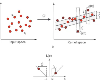
Figure 1 shows an example of an SVR-process in a two-dimensional regression problem, with an
ε-insensitive loss function.
In order to train the above presented model, it is necessary to solve the following optimization prob-lem (Smola and Scholkopf, 2004):
min 12 w 2+ C l
i=1
*
(ξi+ ξi) (3)
subject to
oi− wTϕ(x
i) − b≤ + ξi, i= 1 , . . . ,l (4)
− oi+wTϕ(x
i) + b≤ + ξi*, i = 1 , . . . ,l (5)
*
ξi,ξi ≥ 0, i= 1 , . . . ,l (6)
The dual form of this optimization problem is usually obtained through the minimization of the Lagrange function, constructed from the objective function and the problem constraints. In this case, the dual form of the optimization problem is the following:
max − 12 l *
* *
*
i,j=1(
αi−αi)(αj−αj)K(xi, xj)−
− l
i=1(αi+ αi) + l
i=1 oi(αi − αi)
(7)
l
*
i=1(αi − αi) = 0 (8)
αi,α*i ∈ [0,C] (9)
In addition to these constraints, the Karush-Kuhn-Tucker conditions must be fulfilled, and also the bias variable, b, must be obtained. The interested reader can consult Smola and Scholkopf (2004) for reference. In the dual formulation of the problem the function K(xi, xj) is the kernel matrix, which is formed
by the evaluation of a kernel function, equivalent to the dot product (ϕ[xi], 0[xj]). A usual election for this
kernel function is a Gaussian function, as follows:
Kernel space Input space
xi
* xj
L(e)
Φ
ϕ(xi)
ξi
ξj
ϕ(xj)
+ε
0
–ε
0
*
ξi ξ
j
+ε e
–ε
K(xi, xj) = exp(−γ xi − xj 2). (10)
The final form of function f(x) depends on the Lagrange multipliers αiαi*, as follows:
(x) = l
i=1(αi *
− αi)K(xi, x)
f (11)
In this way it is possible to obtain a SVR model by means of the training of a quadratic problem for a given hyper-parametersC, ϵ and γ. One of the most used free SVR codes is the C implementation of the algorithm described in Chang and Lin (2011), available at https://www.csie.ntu.edu.tw/~cjlin/libsvmtools/.
4. Experiments and results
This section presents the experimental part of the paper. First it is shown how the initial data are prepro-cessed to keep a reduced number of predictive vari-ables for the SVR. The methodology carried out to evaluate the SVR performance is also described in the next subsection. After this, the results obtained by the SVR are presented, together with a comparison with an MLP.
4.1 Data preprocessing and methodology
The input data set is huge, including 100 levels of humidity and temperature from the satellite, TCO measurement (from the previous days to the one to be predicted), aerosol optical depths at seven different wavelengths, and humidity and temperature forecasts (11 different pressure levels: 925, 850, 700, 500, 400, 300, 250, 200, 150, 100 and 50 hPa), from the GFS model. A first prepro-cessing step is needed in order to reduce the size of the data set. This is done by means of a features extraction process using PCA, a technique that has been used before in ozone analysis (Rajab et al., 2013). After this preprocessing step, PCA vari-ables that contain 99.5% of the variance are kept,
which results in a reduced number of variables, as described in Table II.
Since only one year of data is available (see section 2.3), the direct partition of the data into training and test data (as usually performed) could lead to misleading results. Instead, a 20-fold cross validation procedure is proposed, i.e., the available data are split into 20 subsets (with 13 or 14 days per subset), and the performance of the SVR is analyzed by the average that results from training the SVR in 19 subsets and testing in the remaining one.
For comparison purposes an MLP with Lev-enberg-Marquardt training algorithm (Hagan and Menhaj, 1994) is used. MLPs have been previously applied to TCO prediction, and are considered as the state-of-the-art in this field.
4.2 Results
First of all, the performance of the proposed SVR was tested vs. the MLP approach using all variables described in Table II. In addition, to establish the most important features in TCO prediction, both approaches were evaluated using each prediction variable separately. Results are shown in Table III. As can be seen, SVR outperforms MLP in all the cases, with improvements in the range of 5 to 11%. TCO prediction by means of the SVR, considering all the variables, is accurate, with a mean absolute error (MAE) of about 28 Dobson units. TCO prediction, with the input data taken separately, reveals that the accurate prediction of temperatures given by the GFS (10 variables after the PCA pre-processing) is crucial to obtain good TCO predictions. In contrast, neither aerosols and water content (in situ measurements), nor humid-ity given by satellite measurements, contribute to improve the TCO prediction. It is also interesting that the TCO measurement of the previous day is
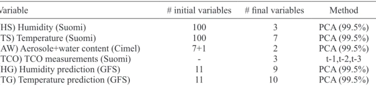
Table II. Input variables considered for TCO prediction after a first data extraction preprocessing step.
Variable # initial variables # final variables Method
(HS) Humidity (Suomi) 100 3 PCA (99.5%)
(TS) Temperature (Suomi) 100 7 PCA (99.5%)
(AW) Aerosole+water content (Cimel) 7+1 2 PCA (99.5%)
(TCO) TCO measurements (Suomi) - 3 t-1,t-2,t-3
(HG) Humidity prediction (GFS) 11 9 PCA (99.5%)
not a very good input variable for predicting TCO for the following day.
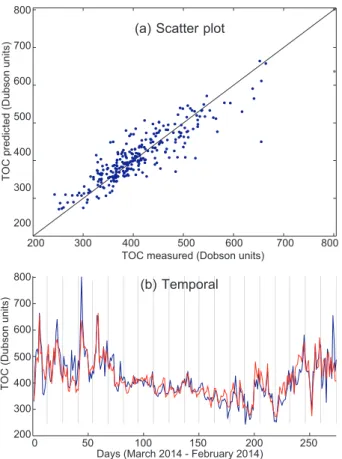
The next issue is whether a subset of data can provide a more accurate TCO prediction than the complete set. Table IV shows the results of using different subsets of predictive variables in TCO prediction. Four subsets are investigated in this case, and compared to the case where all variables are considered. The first subset analyzed is TS + TCO + TG (temperature profiles [Suomi] + TCO measure-ment [Suomi] + temperatures prediction [GFS], in all 20 predictive variables). The second, third and fourth cases are subsets considering combinations of two of these variables. As can be seen in Table IV, TCO prediction using the TS + TCO + TG variables and SVR is the best obtained in all the experiments carried out, with a MAE of about 25 Dobson units. Subsets of two of these variables with the SVR show different behavior: the TCO + TG case (13 predic-tive variables) also gives good results, only slightly inferior to the case with three variables. The third worse case is TS + TG, but it is still better than the TCO prediction obtained considering all variables. Note that the last case (TS + TCO, 10 predictive variables) leads to much poorer results in terms of
TCO prediction, which highlights the importance of the TG variables to obtain a good TCO prediction with a daily time-horizon.
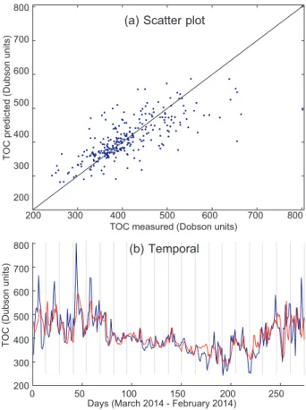
These results can be better visualized by means of depicting TCO prediction graphs. Figures 2, 3, 4 and 5 show TCO prediction using the SVR approach (temporal prediction and scatter plot), corresponding to the predictive variables TS + TCO + TG, TCO + TG, TG + TS and TCO + TS, respectively. Note the good prediction obtained by using SVR with TS + TCO + TG, which follows the TCO peaks and provides a very accurate prediction in all the cases considered. In contrast, the input variables TCO + TS provide a worse TCO prediction, in which the TCO peaks are not completely resolved. This shows the importance of temperature prediction variables (TG) in TCO prediction, and how the rest of the satellite variables provide a slightly more accurate prediction. Note also that humidity variables (either the satellite Table III. Results in TCO prediction (mean absolute
error, in Dobson units) obtained with the different input variables considered.
Variables SVR MLP improvement (%)
all 28.86 31.18 7.44
HS 50.99 56.74 10.13
TS 36.69 41.27 11.09
AW 60.86 65.89 7.63
TCO 41.22 46.71 11.75
HG 44.42 49.33 9.95
TG 30.93 34.57 10.52
Table IV. Results in TCO prediction (mean absolute error in Dobson units) obtained with selected subsets of the input variables considered.
Variables SVR MLP improvement (%)
all 28.86 31.18 7.44
TS+TCO+TG 25.59 28.37 9.79
TCO+TG 26.92 30.02 10.32
TS+TG 27.48 29.93 8.18
TCO+TS 37.85 40.24 5.23
200 300 400 500 600 700 800 200
300 400 500 600 700 800
TOC measured (Dobson units) (a) Scatter plot
(b) Temporal
0 50 100 150 200 250 200
300 400 500 600 700 800
Days (March 2014 - February 2014)
TOC predicted (Dubson units)
TOC (Dubson units)
profile the day before prediction and humidity pre-diction by GFS) do not seem to be relevant variables for obtaining accurate daily TCO predictions.
5. Conclusions
The prediction of total column ozone (TCO) is a difficult problem with important environmental applications. In this paper, a novel and efficient prediction method for TCO has been proposed, which includes an excellent performance regression approach (SVR) applied to a set of predictive vari-ables from heterogeneous sources, such as satellite data (Suomi NPP polar satellite), numerical models (GFS) or direct measurements using devices such as sunphotometers. Data from satellite instruments consist of temperature and humidity profiles at different heights, and TCO measurements from the days before the prediction. The GFS model provides predictions of temperature and humidity for the day
of prediction. Alternative measurement data such as aerosol optical depth at different wavelengths are also considered in the system.
This work shows the good performance of the proposed SVR algorithm applied to daily TCO pre-diction, outperforming alternative algorithms such as neural networks.
An analysis of the most suitable input data for TCO prediction has also been carried out in this study. The results show that temperature prediction by a numerical model is the most important variable to be considered in TCO prediction. We have shown that the SVR methodology is able to provide excellent results in daily TCO prediction, better than the previously considered neural networks algorithms. The improve-ment obtained with SVR over the neural networks methodology is in the range of 5 to 11% in all the cases evaluated. We have also shown the importance of a good temperature prediction by numerical models in obtaining accurate TCO predictions, which can be
200 300 400 500 600 700 800 200
300 400 500 600 700 800
0 50 100 150 200 250 200
300 400 500 600 700 800
(a) Scatter plot
TOC predicted (Dubson units)
TOC (Dubson units)
TOC measured (Dobson units)
Days (March 2014 - February 2014) (b) Temporal
Fig. 3. Prediction (scatter plot and temporal prediction) with SVR using the TCO + TG predictive variables (13 variables). (a) Scatter plot; (b) temporal prediction, TCO measured (blue) and predicted (red).
200 300 400 500 600 700 800 200
300 400 500 600 700 800
0 50 100 150 200 250 200
300 400 500 600 700 800
(a) Scatter plot
TOC predicted (Dubson units)
TOC (Dubson units)
TOC measured (Dobson units)
Days (March 2014 - February 2014) (b) Temporal
complemented with satellite measurements to improve even more the accuracy of the prediction results.
Acknowledgments
This work has been partially supported by the project TIN2014-54583-C2-2-R of the Comisión Inter-ministerial de Ciencia y Tecnología (CICYT) of Spain.
References
Antón M., D. Loyola, B. Navascues and P. Valks, 2008. Comparison of GOME total ozone data with ground data from the Spanish Brewer spectroradiometers. Ann. Geo-phys. 26, 401-412, doi:10.5194/angeo-26-401-2008. Anton M., D. Bortoli, M. J. Costa, P. S. Kulkarni, A. F.
Domingues, D. Barriopedro, A. Serrano and A. M. Silva, 2011a. Temporal and spatial variabilities of total ozone column over Portugal. Remote Sens. Environ. 115, 855-863, doi:10.1016/j.rse.2010.11.013.
Anton M., D. Bortoli, P. S. Kulkarni, M. J. Costa, A. F. Domingues, D. Loyola, A. M. Silva and L.
Alados-Arboledas, 2011b. Long-term trends of total ozone column over the Iberian Peninsula for the period 1979-2008. Atmos. Environ. 45, 6283-6290, doi:10.1016/j.atmosenv.2011.08.058.
Brönnimann S., J. Luterbacher, C. Schmutz, H. Wanner and J. Staehelin, 2000. Variability of total ozone at Arosa, Switzerland, since 1931 related to atmospheric circulation indices. Geophys Res. Lett. 27, 22132216, doi:10.1029/1999GL011057.
Chang C. C. and C. J. Lin, 2011. LIBSVM: A library for support vector machines. ACM Tran. Intel. Syst. Tech. 2, 1-27, doi:10.1145/1961189.1961199.
Chattopadhyay S. and G. Bandyopadhyay, 2007. Arti-ficial neural network with back propagation learn-ing to predict mean monthly total ozone in Arosa, Switzerland. Int. J. Remote Sens. 28, 4471-4482, doi:10.1080/01431160701250440.
Chattopadhyay G. and S. Chattopadhyay, 2009a. Autore-gressive forecast of monthly total ozone concentration: a neurocomputing approach. Comp. Geosci. 35, 1925-1932, doi:10.1016/j.cageo.2008.11.007.
Chattopadhyay G. and S. Chattopadhyay, 2009b. Predict-ing daily total ozone over Kolkata, India: skill assess-ment of different neural network models. Meteorol. Appl. 16, 179-190, doi:10.1002/met.97.
Christakos G., A. Kolovos, M. L. Serre and F. Vukovich, 2004. Total ozone mapping by integrating databases from remote sensing instruments and empirical mod-els. IEEE Trans. Geosci. Remote Sens. 42, 9911008, doi:10.1109/TGRS.2003.822751.
Crutzen P. J., 1970. The influence of nitrogen oxide on the atmospheric ozone content. Q. J. Roy. Meteor. Soc. 96, 320-327, doi:10.1002/qj.49709640815.
Crutzen P. J., 1971. Ozone production rates in an oxy-gen-hydrogen-nitrogen oxide atmosphere. J. Geoph. Res. 76, 7311-7327, doi:10.1029/JC076i030p07311. Farman J. C., B. Gardiner and J. D. Shanklin, 1985.
Large losses of total ozone in Antarctica reveal sea-sonal ClOx/NOx interaction. Nature 315, 207-210, doi:10.1038/315207a0.
Hagan M. T. and M. B. Menhaj, 1994. Training feed forward networks with the Marquardt al-gorithm. IEEE Trans. Neural Net. 5, 989-993, doi:10.1109/72.329697.
Holben B. N., T. F. Eck. I. Slutsker, D. Tanré, J. P. Buis, A. Setzer A, et al., 1998. AERONET-A federated instru-ment network and data archive for aerosol characteri-zation. Remote Sens. Environ. 66, 1-16, doi:10.1016/ S0034-4257(98)00031-5.
Fig. 5. Prediction (Scatter plot and temporal prediction) with the SVR using TCO+TS predictive variables (10 variables); (a) Scatter plot; (b) Temporal prediction, TCO measured (blue) and predicted (red).
200 300 400 500 600 700 800 200
300 400 500 600 700 800
0 50 100 150 200 250 200
300 400 500 600 700 800
(a) Scatter plot
TOC predicted (Dubson units)
TOC (Dubson units)
TOC measured (Dobson units)
Jin X., J. Li, C. C. Schmidt, T. J. Schmit and J. Li, 2008. Retrieval of total column ozone from images onboard geostationary satellites. IEEE Trans. Geosci. Remote Sens. 46, 479-488, doi:10.1109/TGRS.2007.910222. Kanamitsu M., J. C. Alpert, K. A. Campana, P. M. Caplan,
D. G. Deaven, M. Iredell, B. Katz, H. -L. Pan, J. Sela and G. H. White, 1991. Recent changes implemented into the Global Forecast System at NMC. Weather Forecast 6, 425-436, doi:10.1175/1520-0434(1991)006<0425:R-CIITG>2.0.CO;2
Khokhlov V. N. and A. V. Romanova, 2011. NAO-induced spatial variations of total ozone column over Europe at near-synoptic time scale. Atmos. Environ. 45, 3360-3365, doi:10.1016/j.atmosenv.2011.03.056.
Krzyścin J. W. and J. L. Borkowski, 2008. Variability of the total ozone trend over Europe for the period 1950-2004 derived from reconstructed data. Atmos. Chem. and Phys. 8, 2847-2857, doi:10.5194/acp-8-2847-2008.
Latha K. M. and K. V. Badarinath, 2003. Impact of aerosols on total columnar ozone measurements. A case study using satellite and ground-based instruments. Atmos. Res. 66, 307-313, doi:10.1016/S0169-8095(03)00026-7. Martínez-Ballesteros M., S. Salcedo-Sanz, J. C. Riquelme,
C. Casanova-Mateo and J. L. Camacho, 2011. Evo-lutionary association rules for total ozone content modeling from satellite observations. Chemom. Intel. Lab. Syst. 109, 217-227, doi:10.1016/j.chemo-lab.2011.09.011.
Molina M. J. and F. S. Rowland, 1974. Stratospheric sink for chlorofluoromethanes: Chlorine atom cat-alyzed destruction of ozone. Nature 249, 820-812, doi:10.1038/249810a0.
Monge-Sanz B. and N. Medrano-Marqués, 2004. Total ozone time series analysis: a neural network model approach. Non-lin. Proc. Geophys. 11, 683-689, doi:10.5194/npg-11-683-2004.
Pinedo-Vega J. L., C. Ríos-Martínez, F. Mireles-García, V. M. García-Saldívar, J. I. Dávila-Rangel and A. R. Salazar-Román, 2014. Trend of total column ozone over Mexico from TOMS and OMI data (1978-2013). Atmósfera 27, 251-260, doi:10.1016/S0187-6236(14)71114-2.
Rajab J. M., M. Z. MatJafri and H. S. Lim, 2013. Com-bining multiple regression and principal component analysis for accurate predictions for column ozone
in Peninsular Malaysia. Atmos. Environ. 71, 36-43, doi:10.1016/j.atmosenv.2013.01.019.
Salcedo-Sanz S., J. L. Camacho, A. M. Pérez-Bellido and E. Hernández-Martín, 2010. Novel deseasonalizing models for improving the prediction of total ozone in column using evolutionary programming and neural networks. J. Atmos. Solar-Terr. Phys. 72, 1333-1340, doi:10.1016/j.jastp.2010.09.021.
Salcedo-Sanz S., J. L. Camacho, A. M. Perez-Bellido, E. Ortiz-García, A. Portilla-Figueras and E. Hernán-dez-Martín, 2011. Improving the prediction of average total ozone in column over the Iberian Peninsula using neural networks banks. Neurocomp. 74, 1492-1496, doi:10.1016/j.neucom.2011.01.003.
Salcedo-Sanz S., J. L. Rojo, M. Martínez-Ramón and G. Camps-Valls, 2014. Support vector machines in engineering: an overview. WIREs Data-Min. Knowl. Discover. 4, 234-267, doi:10.1002/widm.1125. Savastiouk V. and C. T. McElroy, 2005. Brewer
spectro-photometer total ozone measurements made during the 1998 middle atmosphere nitrogen trend assessment (MANTRA) Campaign. Atmos. Ocean. 43, 315-324, doi:10.3137/ao.430403.
Silva A. A., 2007. A quarter century of TOMS total column ozone measurements over Brazil. J. Atmos. Solar-Terr. Phys. 69, 1447-1458, doi:10.1016/j.jastp.2007.05.006. Smola A. J. and B. Scholkopf, 2004. A tutorial on sup-port vector regression. Stat. Comput. 14, 199-222, doi:10.1023/B:STC0.0000035301.49549.88.
Steinbrecht W., B. Hassler, H. Claude, P. Winkler and R. S. Stolarski, 2003. Global distribution of total ozone and lower stratospheric temperature variations. Atmos. Chem. Phys. 3, 1421-1438, doi:10.5194/acp-3-1421-2003.
Stolarski R. S. and R. J. Cicerone, 1974. Stratospheric chlorine: a possible sink for ozone. Canadian J. Chem. 52, 1610-1615, doi:10.1139/v74-233.
Varotsos C., C. Cartalis, A. Vlamakis, C. Tzanis and I. Keramitsoglou, 2004. The long-term coupling between column ozone and tropopause properties. J. Clim. 17, 3843-3854, doi:10.1175/1520-0442(2004)017<3843 :TLCBCO>2.0.CO;2