Escuela T´
ecnica Superior de Ingenieros de Telecomunicaci´
on
Tesis de M´
aster
M´
aster Universitario en Investigaci´
on en Tecnolog´ıas de la
Informaci´
on y las Comunicaciones
Fiber consistency measures on
brain tracts from digital
streamline, stochastic and global
tractography
Autor:
Gonzalo Barrio Arranz
Tutor:
Dr. Santiago Aja Fern´
andez
from
digital
streamline,
stochastic
and
global tractography
Autor:
Gonzalo Barrio Arranz
Tutor:
Dr. Santiago Aja Fern´
andez
Departamento:
LPI
Tribunal
Presidente:
Dr.
Vocal:
Dr.
Secretario:
Dr.
Fecha:
Calificaci´
on:
Resumen del TFM
La tractograf´ıa es el proceso que se emplea para estimar la estructura de las fibras nerviosas del
interior del cerebroin vivo a partir de datos de Resonancia Magn´etica (MR). Existen varios m´etodos de
tractograf´ıa, que generalmente se dividen en locales y globales. Los primeros intentan reconstruir cada fibra por separado, mientras que los segundos intentan reconstruir todas las estructuras neuronales a la
vez, buscando una configuraci´on que mejor se ajusta a los datos proporcionados.
Dichos m´etodos globales han demostrado ser m´as precisos y fiables que los m´etodos de tractograf´ıa
local, para datos sint´eticos. Sin embargo hasta la fecha no hay estudios que definan la relaci´on entre los
par´ametros de adquisici´on de la MR y los resultados de tractograf´ıa estoc´astica o global con datos reales.
Esta t´esis de Master pretende mostrar la influencia de ciertos par´ametros de adquisici´on como el factor
de difusi´on de las secuencias de adquisici´on, el espaciado entre voxels o el n´umero de gradientes en la
variabilidad de las tractograf´ıas obtenidas.
Palabras clave
RM, RMTD, Tractograf´ıa, Estoc´astica, Global, An´alisis de Imagen M´edica
Abstract
Tractography is the process used to estimate the structure of the nervous fibers in the interior of the
brainin vivofrom magnetic resonance data (MR). There are several methods of tractography, which are
usually divided into local and global. The first attempt to reconstruct each fiber separately, while the latter try to reconstruct all the neural structures at the same time, looking for a configuration that best fits the provided data.
However to date there are no studies that define the relationship between MR acquisition parameters and the results of stochastic or global tractography with real data.
This Master thesis is intended to show the influence of some parameters of acquisition as the factor of dissemination of sequences of acquisition, the spacing between voxels or the number of gradients in the variability of the obtained tractographies.
Keywords
Agradecimientos
Contents
1 Introduction 1
1.1 Basis of MRI and tractography . . . 1
1.1.1 Basis of DTI mathematical model . . . 1
1.1.2 Basis of tractography . . . 1
1.2 Objectives . . . 2
1.3 Phases and methods . . . 2
1.4 Structure of this memory . . . 3
2 Study plan 5 2.1 Objectives for data processing . . . 5
2.1.1 Tractography algorithms . . . 5
2.1.2 Profile extraction from fiber tracts . . . 5
2.1.3 ROI definition and spatial filtering . . . 5
3 State of Art 11 3.1 Diffusion Weighted Imaging (DWI) . . . 11
3.2 Diffusion Tensor Imaging (DTMRI) . . . 11
3.3 Low and high-order diffusion models . . . 12
3.3.1 Spatial model approaches . . . 12
3.3.2 Q-space model approaches . . . 13
3.3.3 Mixture model approaches . . . 15
3.4 Tractography: Basics . . . 17
3.4.1 Deterministic algorithms . . . 17
3.4.2 Probabilistic algorithms . . . 21
3.4.3 Global optimization algorithms . . . 25
3.4.4 Other tractography algorithms . . . 27
3.5 Limits of neural tractography . . . 27
4 Materials and methods 31 4.1 Materials . . . 31
4.1.1 Patients and data acquisition . . . 31
4.2 Methods . . . 31
4.2.1 Tensor estimation . . . 31
4.2.2 Tractography process . . . 32
4.2.3 Stochastic tractography algorithm . . . 33
4.2.4 Global tractography parameters . . . 33
4.3 Spatial Filtering . . . 34
5 Software additions to Saturn (Software Application of Tensor Utilities for Research in Neu-roimaging) 35 5.1 Introduction . . . 35
5.2 Additions in the GUI . . . 36
5.3 New tools . . . 36
5.3.2 Fiber deleting tool . . . 38
5.3.3 Deleting fibers by size . . . 39
5.3.4 Spatial filtering methods based on ROIs . . . 39
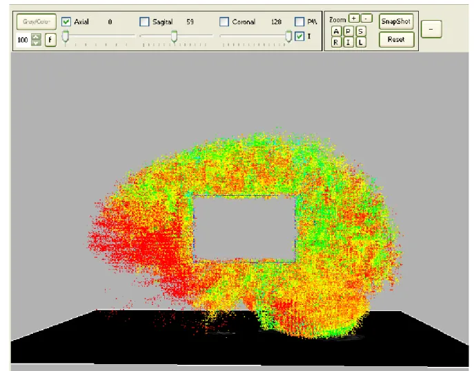
5.3.5 Fiber visitation map creator . . . 39
5.3.6 Random seed tractography tool . . . 40
5.3.7 Profile extractor for fiber tracks . . . 41
5.3.8 Superresolution track density imaging method . . . 41
6 Results 43 6.1 Reproducibility studies . . . 43
6.1.1 Reproducibility of the Corpus Callosum . . . 43
6.1.2 Reproducibility of the Left Cingulum . . . 49
6.1.3 Reproducibility of the Right Cingulum . . . 50
6.2 Profile comparison studies . . . 50
6.2.1 In Corpus Callosum . . . 51
6.2.2 In Left and Right Cingulum . . . 51
6.3 Discussion of the results . . . 54
6.3.1 Effects of SNR . . . 54
6.3.2 Variance differences between global and streamline tractography . . . 54
6.3.3 Effect of b-values . . . 56
6.3.4 Effect of the number of gradients . . . 56
6.3.5 Effects of spatial resolution . . . 56
7 Conclusions 57 7.1 Future lines of investigation . . . 57
A Publications of this Master thesis 63
B Connectivity data tables 69
List of Figures
2.1 ROIs defining IOFF spatial filter. . . 6
2.2 ROIs defining Cingulum spatial filter. . . 7
2.3 ROIs defining CST spatial filter. . . 8
2.4 ROIs defining CC spatial filter. . . 8
3.1 Schematic view of a myelinated axon [13]. . . 11
3.2 ODF estimation with DSI [48]. . . 13
3.3 Illustration of the grid sampling and the spherical sampling acquisition protocols [48]. . . 14
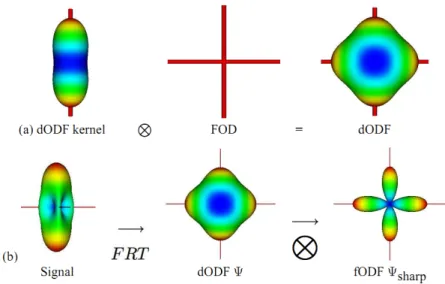
3.4 Spherical convolution / deconvolution. In a) the convolution between diffusion ODF (dODF) kernel and the fiber orientation distribution (FOD) produces a smooth dODF. In b) the Funk Radon transform (FRT) of the simulated HARDI signal produces a soomth dODF; which is transformed into a sharp fiber ODF by a deconvolution with the ODF kernel of a) [20]. . . 16
3.5 Fiber path composed by a track of vectors [38]. . . 17
3.6 An example of deterministic tractography. . . 18
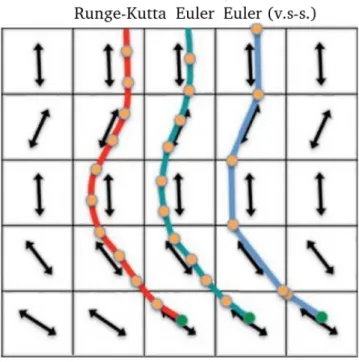
3.7 Three track propagation algorithms. From left to right: Runge-Kutta, Euler and Euler with variable step-size. . . 20
3.8 An example of probabilistic tractography [38]. . . 22
3.9 Synthetic data of five equal FA paths. There is a bias that favors shortest, straightest paths [47]. . . 24
3.10 Two line segments (given by midpoints x1, x2 and orientations n1, n2) and the elements for con-structing their internal energy. The red dotted lines indicate the distances whose sum of square defines the internal energy [56]. . . 26
3.11 ODF estimation for different complex fiber configurations [48]. . . 28
5.1 Additions to the GUI. . . 35
5.2 Flip DWI loading directions. . . 36
5.3 Interactive fiber selection. . . 37
5.4 Delete fiber tool panel. . . 38
5.5 Interactive fiber deleting tool. . . 38
5.6 Delete fibers by distance panel. . . 39
5.7 Fiber filter by ROI panel. . . 39
5.8 Example of fiber visitation map. . . 40
5.9 Random seed example. . . 41
5.10 Profile extractor panel. . . 41
5.11 Profile map example for two different tractography methods, left -global tract, right -streamline tract. 42 5.12 Superresolution TDI example. . . 42
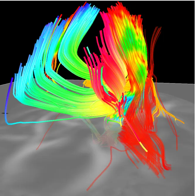
6.1 Reconstructed fibers with Global tractography. . . 44
6.2 Reconstructed fibers with Streamline tractography. . . 45
6.3 Normalized fiber count, Corpus Callosum, for global t.(up) and streamline t.(down). . . 46
6.7 Standard Deviation of FA from the fiber profiles separated by patients, Global t., Corpus Callosum. 51
6.8 Standard Deviation of FA from the fiber profiles separated by patients, Streamline t., Corpus Callosum. 51
6.9 Standard Deviation of FA from the fiber profiles, Global(up) and Streamline t.(down), Corpus
Callosum. . . 52
6.10 Standard Deviation of FA from the fiber profiles separated by patients, Global t., Left Cingulum. . . 53
6.11 Standard Deviation of FA from the fiber profiles separated by patients, Streamline t., Left Cingulum. 53
6.12 Standard Deviation of FA from the fiber profiles separated by patients, Global t., Right Cingulum. . 53
6.13 Standard Deviation of FA from the fiber profiles separated by patients, Streamline t., Right Cingulum. 54
Chapter
1
Introduction
1.1 Basis of MRI and tractography
Magnetic Resonance Imaging (MRI) is a medical imaging technique used to visualize the internal structures of
the bodyin vivo. MR images are extremely rich in information due to the great number of parameters that have
influence on each voxel value. One of its main features is that we can use it to differentiate between tissue types, and it has been very successfully as a diagnostical tool, but it is not an adequate tool to study the intricacies of the structure of the nervous tissues.
Diffusion Tensor Imaging (DTI) can solve this limitation [1]. DTI is a MRI method that maps the diffusion process of the water molecules, providing information about the diffusion of water at each voxel. Molecular diffusion in tissues is not free, and reflects interactions with many obstacles around it. For example, the neural axons of white matter in the brain or muscle fibers in the heart have an internal fibrous structure. Water will then diffuse more rapidly in the direction parallel to the fibers, and more slowly perpendicular to it, therefore revealing details about tissue architecture, either healthy or diseased.
Some neurological diseases are associated with abnormalities that can be detected an measured with DTI
1.1.1 Basis of DTI mathematical model
Each voxel contains information about the local characteristics of diffusion. Normally, this information is modeled as a 2nd order tensor, using measurements from at least six different directions.
Modeling diffusion as a tensor has certain mathematical advantages, they are rotationally invariant ( their values does not change when the coordinate system used to describe them is rotated ); the diffusion tensor is positive definite, thus all of its eigenvalues are positive. Each eigenvalue represents the magnitude of diffusion in the direction of the eigenvector associated with that eigenvalue.
The 2nd order tensor can be described as an ellipsoid, whose major and minor axis are formed by the eigenvectors and associated eigenvalues of the tensor. The eigenvector associated with the largest eigenvalue is sometimes referred to as the principal diffusion direction.
1.1.2 Basis of tractography
But the tensor and its eigenvalues and eigenvectors are a multidimensional structure and is not useful to visualize the interior of the brain. A popular technique used to visualize these diffusion tensors is to extract fiber tracts which summarize the diffusion information across many voxels. This technique is known as tractography.
Several methods exist for performing tractography:
The most common method is to generate fiber tracks that follow the direction of maximal water diffusion
Stochastic tractography [38] provides a measure of confidence of the estimated fiber tracks, by performing tractography under a probabilistic framework. They can generate tracts that momentarily pass through regions of low anisotropy because they integrate local fiber orientation uncertainty into the uncertainty of the entire tract.
Global tractography methods try to reconstruct the fibers simultaneously by finding the configuration that
describes best the measured data. Global tracking promises a better stability with respect to noise and imaging artifacts.
The fibers are reconstructed from small line segments that get bind together during the optimization phase. Their orientation and number are adjusted simultaneously to match the data.
The main problem of global methods is a very long computation time, often unacceptable in the clinical setting.
Together, DTI and tractography can help us to study the structure of the brain and to obtain quantitative measures of diffusion within its tissues. They work particularly well in defining and characterizing white matter structures. it exists a growing interest in the last decades in using magnetic resonance diffusion imaging to provide information on anatomical connectivity in the brain by measuring the diffusion of water in white matter tracts. Among the measures, the most commonly derived from diffusion data is fractional anisotropy (FA), which quantifies local tract directionality and integrity.
But while DT-MRI tractography can produce striking images of the brain anatomy, it suffers from a number of problems:
Brain tractography lacks of a neuroanatomical white matter ”gold standard”. Currently it does not exist
a definitive validation standard for in vivo images.
Lack of reliability within the same data-set. For many tractography algorithms, specially for the simple
streamline methods, their estimations are very dependent on seedpoint placement. Also, there can be differences based on the initialization position. The propagation of fibers through a noisy diffusion tensor field may result in deviation from the true fiber and therefore may lead to erroneous connection estimates. The errors in the diffusion tensor and, consequently, the major eigenvector are an unknown function of the measurement noise, tensor eigenvalues, tensor encoding set, and tensor field geometry. There can be even computer-dependent bias.
Problems resolving the crossing or meeting of different fiber bundles
In summary, obtaining reliable data and drawing meaningful and robust inferences from them, with diffusion MRI, can be challenging. The effects of the acquisition parameters on the quantifying diffusion indexes, have been profusely studied; some papers such as Wakana et al.[71] have studied the effects of streamline reproducibil-ity intersubjects and intrasession, and Zhan et al.[73] have studied the effects of some acquisition parameters onto streamline connectivity but the effects of the acquisition parameters into the reproducibility of different tractography algorithms have not been properly studied.
1.2 Objectives
One of the ultimate goals for all tractography techniques is to define quantitative and reproducible parameters for measuring anatomical connectivity. The main objective of this Master’s thesis is to study the reproducibility of the fiber tracks and the variability created by the acquisition parameters onto the reconstructed fiber tracks for different tractography methods. To evaluate which of the the major technical factors of DTI that affect image quality also have effect in the track results; with a special focus on the b-values, the number and orientations of diffusion-weighted acquisitions, voxel spacing as well as the fiber tracking parameters
1.3 Phases and methods
The following phases are followed for the writing of this Master thesis:
1 Reading literature on the scope of the project; as a contact intake with the properties and essential concepts.
2 Study of existing algorithms currently used in the state-of-the-art tractography.
1.4 Structure of this memory
This report has been structured in seven chapters:
Chapter 2 establishes the basis of our experiments.
Chapter 3 discusses the theoretical concepts and general ideas behind MRI and the DT-MRI, and gives
an state of the art of the the mathematical models used to characterize the diffusion and its use along the main existing tractography methods and algorithms.
Chapter 4 details the materials and methods used in the experiments, explaining the parameters and
configurations employed.
Chapter 5 explains the additions created for the Saturn software (Software Application of Tensor Utilities
for Research in Neuroimaging) specifically for this Master thesis.
Chapter 6 collects the results obtained for the tractography experiments and discuses them.
Chapter 7 finally details the conclusions of this work and possible future lines of investigation.
Chapter
2
Study plan
The objective of this study is to understand how the acquisition parameters of the MR can influence the tractogra-phy results. In order to accomplish this, we want to compare tractogratractogra-phy reconstructions of different parts of the brain, created with different tractography methods, from several volume data acquired with three combinations of three different acquisition parameters.
In order to compare the tracks, we plan to check two different factors: The count of correctly extracted tracks and the mean profiles extracted from the fibers. There are many potential sources of variation in quantitative DTI parameters. Therefore, is important to be consistent in data acquisition, reconstruction, and processing across subjects in clinical DTI research.
2.1 Objectives for data processing
One of the major sources of variability of the track estimation, in addition to noise and lack of spatial resolution, comes from the fact that fiber tracks have to be started from certain user-selected ROIs to identify specific white matter tracts. This fact can be avoided by seeding every voxel in the entire 3D volume containing the head, and thereby generating all the white matter streamlines in one computation. Then, we can extract specific tracks by using manually placed ROIs and spatial designed filters. This process is known as whole brain tractography.
Whole brain tractography as two main advantages over the more simple user-selected ROI points. First is an automatic process; second, it may find some tracks that are missed by ROI-based seeding; third, the large number of fibers created can compensate small error estimation that accumulates along each step of the tractography and finally it can produce a better balance of streamline density along the delineated tract. On the flip side, it has great requirements of computation time, memory and disk space.
2.1.1 Tractography algorithms
We plan to compare two local tractography algorithms and one global: The streamline tractography proposed by Mori et al.[22], a bayesian probabilistic algorithm implemented by Friman et al.[38]. and a global reconstruction algorithm implemented by Reisert et al.[56].
2.1.2 Profile extraction from fiber tracts
Profiles of each fiber are extracted based from their points, limited from a max distance to a preestablished model. Mean values and standard deviation of the tensor values are computed and stored. Tract based measurements are more robust and reproducible than voxel-wise measures, in both intrasession and intersession measurements, according to Farrel et al.[70]
2.1.3 ROI definition and spatial filtering
Figure 2.1: ROIs defining IOFF spatial filter.
brain, even in regions with highly coherent fibers, due to noise, distortions in the DTI data or insufficient spatial resolution which result in partial volume effects. To avoid highly isotropic regions, our experiments are centered on highly anisotropic and well known regions of the brain.
For this work, we are interested in four major white matter structures, the Inferior Occipitofrontal Fasciculus (IOFF), the Corpus Callosum (CC), the Cingulum (Cing) and the Corticospinal tract (CST). These are highly studied brain zones, with a high number of connections and a very defined main orientation.
Inferior occipito-frontal fasciculus (ioff)
This white matter structure crosses the brain along the Anterior to Posterior axis. Connects the ipsilateral frontal and occipital lobes; ipsilateral frontal and posterior parietal and temporal lobes; intermingles with uncinate fasciculus. Its main function is the integration of auditory and visual association cortices with prefrontal cortex. It is also related with the language learning.
On the RGB viewer, these fibers are easy to identify ( they are marked in green in the fig. refIOFF ) as they cross the brain from the Anterior to the Posterior part of the brain. Two groups of three ROIs are defined to filter the the left and right IOFF fibers:
First, from the Sagittal view on the left hemisphere, we define a small patch over the middle occipital surcus
( a hook shaped curve on the Parietal region ). This is shown on the fig. 2.1.3 (right).
Then, again from the Sagittal view, define the other two regions, on the Central and the Anterior regions,
as can be seen on the fig. 2.1.3 (center and left).
Changing to the Coronal view, we search the ROIs that we have defined and complete them. This is shown
on the fig. 2.1.3 ( left, center and right ).
We repeat these three steps for the other side of the brain.
Cingulum
Figure 2.2: ROIs defining Cingulum spatial filter.
First, from the Axial view, we define the first region on the just over the Corpus Callosum ( shown on the
fig. 2.1.3 left ).
The second ROI is defined form the Sagittal view; at the same level of the previous ROI, both at the front
and the back of the Corpus Callosum limits ( seen the fig. 2.1.3 (center) ).
The third ROI follows the inferior part of the gyrus. The ROI does not follow the same straight direction
of the superior part, but turn outwards to the temporal lobe. This ROI can be seen on the fig. 2.1.3 ( right ).
Finally, from the Axial view, we must search the previously defined ROIs and complete them.
Corticospinal tract
This region connects the cerebral motor cortex to medulla, then descends into contralateral spinal cord. The corticospinal tract conducts impulses from the brain to the spinal cord. It contains mostly motor axons. The corticospinal tract is made up of two separate tracts in the spinal cord: the lateral corticospinal tract and the anterior corticospinal tract. If injured, induces motor deficiencies and hemiparesis. The corticospinal tract originates from pyramidal cells in layer V of the cerebral cortex. About half of its fibres arise from the primary motor cortex. Other contributions come from the supplementary motor area, premotor cortex, somatosensory cortex, parietal lobe, and cingulate gyrus. The average fiber diameter is in the region of 10 micrometers.
These ROIs are defined from the Axial and Coronal views. The Corticospinal Tract can be seen on the RGB viewer in blue, from the base of the spinal cord to the blue-green at the somatosensor cortex:
The first ROI is defined from the Axial view, covering all the base of one side of the medulla( as is shown
on the fig. 2.1.3 left ).
The second ROI is first defined on the Coronal view; at the same Anterior to Posterior level that the
previous ROI. This new ROI must be situated at the height of the internal capsule. Then, from the Axial view, we complete the ROI of the fiber tract. An example can be seen on the fig. 2.1.3 (center).
The third ROI is first defined from the Coronal view at the same A-P level of the previous ROIs, and covers
all the motor area of the cortex. The figure 2.1.3 right shows an example.
Figure 2.3: ROIs defining CST spatial filter.
Corpus Callosum
The Corpus Callosum is the largest fiber bundle in the brain. It connects the neocortical areas between both cerebral hemispheres; most are mirror image of each other. It is related to interhemispheric sensorimotor function and auditory connectivity.
The CC is a wide, flat bundle of neural fibers beneath the cortex in the eutherian brain at the longitudinal fissure. It connects the left and right cerebral hemispheres and facilitates interhemispheric communication. It is the largest white matter structure in the brain, consisting of 200-250 million contralateral axonal projections.
The ROIs for the Corpus Callosum are defined from the Sagittal and the Axial views. The Corpus Callosum can be seen on the RGB viewer in red at the level of the interhemispheric fissure, turning to blue up to the superior and parietal cortex. The protocol used to define the ROIs is this:
The first ROI is defined from the Sagittal view, at the center of the brain, at the level of the interhemispheric
fissure,. The Corpus Callosum is the big red zone that goes between the brain hemispheres from left to right ( as is shown on the fig. 2.1.3 left ).
The second ROI and third ROI are defined form the Axial view; one over the right and one over the left
Chapter
3
State of Art
3.1 Diffusion Weighted Imaging (DWI)
Diffusion Weighted Imaging (DWI) is a non invasive technique of Magnetic Resonance (MR) that provides infor-mation about the the diffusion of water molecules in the brain. This technique appeared first in the late 1980s
and it is used to study the local characteristics of water molecules inside organic tissuesin vivo.
Its physical basis is the assumption that the phase of the electrons of the water molecules inside the biological tissues respond at intense magnetic fields ( for example, in a typical T1-weighted image water molecules are excited with a strong homogeneous magnetic field ). In T2-weighted images, contrast is produced by measuring the loss of synchrony between the water protons. When water is in an environment where it can freely tumble, relaxation times tends to take longer. Using this data, we can create an image that differentiates between tissue types due to their relaxation time.
Unfortunately, MRI images do not provide much information about the orientation of the neural tracts within each voxel; information we could use to determine the connectivity between different regions of gray matter.
These interactions are orientation-dependent, meaning that the diffusion in parts of the brain has directionality. The influence of several magnetic fields from different orientations is useful for determining structures in the brain that restrict the flow of water in one direction, such as the myelinated axons of nerve cells. As the Figure 3.1 shows, the myelin cover and the neurofilaments are oriented structures that cause the perpendicular diffusion
coefficient, D(⊥), to be smaller than the parallel diffusion coefficient D(k). Knowing the main structure and
Figure 3.1: Schematic view of a myelinated axon [13].
connectivity of the brain, and differences between health and pathological tissues can give us a great insight of the neural diseases and of the brain itself.
3.2 Diffusion Tensor Imaging (DTMRI)
by a pulsed field gradient. Since precession of the protons is proportional to the magnet strength (b-value), they move at different rates, resulting in dispersion of the phase and signal loss. Then, another gradient pulse is applied ( with the same direction and opposite magnitude ) to refocus or rephase the spins. Protons that have moved between pulses due to Brownian diffusion reduce the signal measured by the MRI machine. Therefore each DWI provides information about the magnitude of diffusion in one particular direction. Using from six to, sometimes, hundreds of measurements is possible to generate a single resulting calculated image data set [1].
In DTI, each voxel is defined by its rate of diffusion and its preferred direction of diffusion. These properties
are described by a 3×3 symmetric tensor with six uniques coefficients.
The properties of each voxel of a single DTI image is usually calculated by vector or tensor math from six or more different diffusion weighted acquisitions, each obtained with a different orientation of the diffusion sensitizing gradients.
Under noise-free conditions, the diffusion tensor is related to the DWI intensity by this equation:
Si=S0e−big
T
iDgi (3.1)
where D is the diffusion tensor, Si is the DWI intensity, S0 is the baseline intensity, gi and bi are the
gradi-ent directions and diffusion weighting factor respectively. The diffusion tensor is positive definite, so all of its eigenvalues are positive. Each eigenvalue represents the magnitude of diffusion in the direction of the eigenvector associated with that eigenvalue. The eigenvector associated with the largest eigenvalue is also called the principal diffusion direction (PDD). Some anisotropy coefficients that can be derived from the tensor information, such as Fractional Anisotropy (FA) and others, can be used in clinical studies [3].
The single diffusion constant is the simplest model that we can use to characterize water diffusion, assuming that the system has isotropic structures. Its main advantage (simplicity, as it only needs six parameters to be estimated) can also be its main weakness. The tensor model may oversimplify the underlying anatomy,so it is important to interpret results derived from the tensor model with care. For these reasons, there is an increasing interest in high order models that can capture and display the DWI information.
Ultimately, clinical researchers are often interested in the global neural fiber bundles. These span through multiple voxels, limiting the usefulness of localized studies. The directional information can be exploited at a higher level of structure by following neural tracts through the brain. This process is called tractography.
Most of the current techniques in DWI tractography can be divided into two major components: local
modeling of the diffusion propagatorat each voxel, andfiber tracking algorithmsintegrating this local information into streamlines representing fiber tracts. Advanced tractography algorithms and high-order models are key concepts in the study of neural structures and its connectivity; and both are highly related to each other. In the next sections we will describe them in detail.
3.3 Low and high-order diffusion models
The role of the modeling techniques is to reconstruct the diffusion propagator from DWI data; converting the diffusion weighted signal into a quantity able to characterize the number and orientation of the fiber tracts at each voxel.
Some methods try to simplify the reconstruction of the diffusion propagator; either on the spatial domain or on the q-space acquisition domain. The first works under the assumption of Gaussian anisotropic diffusion and is simpler; the second provides a less parametrized representation of the diffusion propagator. More complex models use composited acquisitions, like the multiple-tensor model and the ball-and-stick model.
Also, another class of methods directly aims to the reconstruction of the distribution of fiber orientations, e.g., by spherical deconvolution.
3.3.1 Spatial model approaches
Simple diffusion tensor model
DT assumes that diffusion model is a mean zero trivariate Gaussian distribution.
p(x) =`
(4πt)3det(D)´−12exp
„
−x
T
D−1x
4t
«
(3.2)
D is the diffusion tensor and t the diffusion time.
D=
0 @
Dxx Dxy Dxz
Dyx Dyy Dyz
Dzx Dzy Dzz
1
A (3.3)
DTI is popular due to the simplicity of the model and of the imaging acquisition. Also is compatible with clinical conditions. However, it can only characterize one fiber compartment per voxel; this simplification is not always a good representation of fiber orientation and can lead to difficult interpretations in complex regions.
Several alternatives have been proposed to overcome the DT limitation, most of them are based on high angular resolution diffusion imaging (HARDI), which uses several tens to a few hundreds of DWI.
3.3.2 Q-space model approaches
Methods based on q-space provide an estimate of the angular dependence of the spin propagator, by exploiting its Fourier relationship with the DWI signal measured as a function of the q-vector [2]. The estimated spin propagator corresponds to the probability that a random water molecule will have a particular displacement over the diffusion time. In these models the fiber orientation are taken from the spin propagator by identifying the directions along which the probability of displacement is highest.
A common criticism of the q-space methods is the violation of the Narrow Pulse Approximation ( the as-sumption that the spins move an insignificant distance during the gradient pulse itself ). Q-space formalism is
only strictly valid if this condition is true, and for thein vivo cases, this requires DW gradient pulse durations
of 1 ms or less. Unfortunately, on current clinical systems, the required diffusion weighting cannot be obtained with such short pulse durations due to the limited gradient amplitudes available. However, it has been shown that with longer DW gradient pulses, the spin displacements obtained reflect the difference between the spin’s time-averaged positions during each DW gradient pulse. This will cause an underestimation of quantitative mea-surements of displacement, but importantly will not necessarily affect the estimated orientations, and indeed may be beneficial[4],[5].
Another criticism of q-space is the fact that the directions with the highest probability of displacement are relatively broad and overlap significantly. While not necessarily a problem itself, closely aligned fiber orientations will be blurred together and will thus be identified as a single orientation; this can lead to a bias in the estimated fiber orientations [6].
Figure 3.2: ODF estimation with DSI [48].
Diffusion Spectrum Imaging (DSI)
DSI is the direct application of q-space in 3D. It reconstructs a discrete representation ofp directly from a 3D
the diffusion orientation density function (ODF) frompas:
ODF(ˆx) =
Z inf 0
p(αxˆ)dx (3.4)
where ˆxis a unit vector in the direction of x. The reconstruction gives the values ofpon a grid of displacement.
Fiber orientations are identified by reducing the 3D spin propagator to its 2D radial projection and finding
the peaks of its ODF.ODF(ˆx) is computed numerically by interpolating the grid representations ofp:
For a 3D vector~uwith|u|= 1, we define
ODF(u) =
Z
p(ρu)ρ2dρ (3.5)
where ρ =|r|,ρ2dρ is the 3D volume element and the integral is computed as a discrete sum over a range of
voxels in diffusion r-space. The ODF can have multiple pairs of equal and opposite peaks, each pair provides a distinct fiber orientation estimation. The figure 3.5 shows the procedure: on the left panel, the white spots shows
the points in which we acquire the measurements; the second panel showsp, the Fourier Transform of the signal,
together with the grid displacement vectors at which the FFT provides the value of p. To obtain the ODF we
interpolate the grid of samples ofpand integrate along radial lines.
The main disadvantages of DSI are:
Requires a large amount of data ( the complete Cartesian sampling of q-space), at least one order of
magnitude greater than DT.
Lengthy acquisition (requires large pulsed field gradients to satisfy the Nyquist condition for diffusion in
nerve tissue).
This measurement scheme is not practical if we are only interested on the angular structure (much of the
infor-mation in the measures contributes only to the radial structure ofp).
Q-Ball Imaging (QBI)
An alternative approach to DSI, based on sampling on a spherical shell (or combination of shells) in diffusion wavevector space, as seen in figure 3.3.2,. Uses shorter acquisition times and requires less data than DSI. It approximates the ODF using a spherical tomographic inversion called the Funk-Radon transform (also known as
the spherical Radon transform). The value of the transformation of a spherical function at a point ˆxis the integral
Figure 3.3: Illustration of the grid sampling and the spherical sampling acquisition protocols [48].
of the function over the circleC(x) perpendicular to ˆxat a fixed radius in q-space. Is model-independently and
Persistant Angular Structure (PAS)
In [12], Jansons et al. define, for the HARDI data, a statistic called the (radially) persistent angular structure (PAS). It is a representation of the relative mobility of particles in each direction. Spins are assumed to diffuse a fixed distance with an angular distribution given by the PAS. The spherical samples in the q-space of the 3D Fourier transform can be taken as the probability density function of particle displacements.
It is a computationally intensive method. The non linear optimization and numerical integration make the PAS much slower than QBI or deconvolution methods, so normally a maximum entropy constraint is defined to operate on low b-value data and to improve the stability of the results and the velocity of its estimation.
Both QBI and PAS compute functions of the sphere that reflect the angular structure of the particle displace-ment density. The peaks of these functions provide estimates of fiber orientations.
Diffusion Orientation Transform (DOT)
Like PAS, it gives an estimation of a spin propagator at any given radius. The 3D Fourier transform is made tractable by assuming a mono exponential radial dependence for the DW signal. ODF is not a radial projection
of the spin propagator, but corresponds to the amplitude of the spin propagator for a chosen displacementR0.
This provides increased separation between various fiber orientations when using larger values ofR0.
3.3.3 Mixture model approaches
Mixture models assume that the DW signal for a particular combination of fiber orientations is the weighted sum of each population’s contribution to the signal.
Estimating the fiber orientations becomes a matter of fitting the model to the given DW data.
This requires two conditions: first, there is a negligible exchange of water molecules between fiber populations at diffusion time ( according to [13] exchange effects can only become significant if fibers from different bundles interdigitate at micron scale ) and second, fibers must share at least some of the DWI characteristics, which makes possible to reduce the complexity of the model and increase the stability of the reconstruction ( this can go from assuming axial symmetry of diffusion to stating that the diffusion signal is identical for all fiber bundles ). These assumptions may seem excessive, but these parameters have a relative weak effect on anisotropy and the estimated orientation will not be affected by it.
Mixture models can be improved with constraints: i.e. those based in prior knowledge of the fiber distribu-tion (like the constraint of non negative volume fracdistribu-tions [9]) or a maximum entropy constraint (that favors a distribution of fiber orientations with a few well defined peaks [10]).
Multi tensor model
A natural extension of the DT model. Assumes that the DWI signal is created from a mixture of compartments
each described by its own diffusion tensor. The signalS(g) is predicted as the combination of several Gaussian
models:
S(g) =S0
n
X
i=1
fiebg
TD
ig (3.6)
where n is the number of compartments, S0 is the non diffusion-weighted signal, b is the diffusion weighting,
and g is the diffusion-sensitizing gradient. The sum offi is equal to one. There are particles displacements inn
distinct compartments, between which no exchange of particles occurs. It is assumed that the number of distinct
fiber populations is known. A full n-tensor model has 7n−1 degrees of freedom, but additional constraints are
imposed in practice. Usually, by assuming equal eigenvalues on allDi, or imposing axial symmetry (l2 =l3 ).
For practical considerations of noise, most works normally uses a maximum of n= 2 (losing accuracy if it fits a
model withn≥2 ).
Figure 3.4: Spherical convolution / deconvolution. In a) the convolution between diffusion ODF (dODF) kernel
and the fiber orientation distribution (FOD) produces a smooth dODF. In b) the Funk Radon transform (FRT) of the simulated HARDI signal produces a soomth dODF; which is transformed into a sharp fiber ODF by a deconvolution with the ODF kernel of a) [20].
Combined Hindered and Restricted Model of Diffusion (CHARMED)
CHARMED is strongly related to multitensor models. It is formed by one extra axonal compartment (
char-acterized by a single diffusion tensor ) andn intra-axonal compartments ( corresponding tonfiber populations
).
It is characterized by a model of restricted diffusion within cylinders. Requires a more complete 3D q-space acquisition to discriminate between both models. In CHARMED, the data is acquired from multiple q-values per DW orientation, and multiple orientations. Also this model requires a large maximum q-value ( accomplished by increasing echo acquisition time . By contrast, most high-order models employs the HARDI strategy: acquiring a large number of DW directions with a constant b or q-value. This allows to focus on the angular part of the DW signal and to select the most appropriate diffusion weighting to maximize contrast to noise per unit of scan-time [14].
Ball and stick model
This model assumes that all Di have equal eigenvalues ( completely isotropic ) and the remaining “stick”
com-partments are perfectly linear ( the second and third eigenvalues are zero l2 =l3 = 0). For nfiber terms, this
leads tok=n+ 1 compartments and 3n+ 1 degrees of freedom. We consider the model up ton= 3. Fitting the
ball-and-stick model can theoretically be formulated as a deconvolution problem with a discrete ODF
Spherical Deconvolution model(SD)
A generalization of previous methods: SD assumes a distribution, rather than a discrete number, of fiber popu-lations. The summation becomes an integral over the distribution so it takes account for an infinite number of
fiber populations. The method assumes that the diffusion signalS(θ, φ) is the convolution of the ODF.
It tries to reconstruct directly the distribution of fiber orientations. This requires an explicit model of the diffusion properties of a single fiber ( convolution kernel ), and its results are more easily interpretable.By assuming a particular convolution kernel ( representing the DW signal for single fiber orientation ) the fiber orientation distribution can be estimated by a constrained spherical deconvolution.
S(θ, φ) = 2π
Z
0
π
Z
0
where γ0 is the angle between directions given by (θ, φ) and (θ0, φ0). Typically,S(θ, φ) andR(γ) are estimated from the data and modeled in spherical harmonics and rotational harmonics, respectively. This reduces spherical
deconvolution to simple scalar division, and yieldsODF(θ, φ).
Some implementations differ in the convolution kernel employed ( some assume a DT model [15], and some measure it directly from the data [16] ). They also differ in the constraints of the solution (some implementations introduce a non negativity constraint [16] and others a maximum entropy term [10] ).
SD, like DSI and QBI, can be expressed as linear matrix operations, so their computation times can be kept very short. Linear spherical deconvolution is extremely fast and does not require pre-specification of an expected number of fibers. On the other hand, multi-tensor models offer higher accuracy for applications like multi-fiber streamline tractography.
3.4 Tractography: Basics
In the brain, the white matter consist in axons that form bundles which connect different regions of the brain. Fiber tractography algorithms take the local diffusion information and integrate them into tracks that aim to represent the neural fibers tracts. Many prominent tracts are large enough to be delineated by DTI and to estimate connections between adjacent voxels.
Tractography is the only tool we currently have to visualize white matter neural tracts in vivo and non
invasive, providing us information of the white matter architecture and connections.
The most simplest implementation for performing tractography is the numerical integration between neigh-boring image voxels that are thought to belong to the same white matter fiber tract. Typically, it starts from a preassigned voxel called the “seeding voxel”. Integration continues examining the directional consistency between the principal eigenvectors of the two neighboring voxels and between the fiber direction and the vector connecting
the two voxels. The angleθbetween two vectorsaandbcan be calculated with the inner product:
cos(θ) = ~a~b
|~a~b| (3.8)
Knowing the angular relationships, tractography continues choosing those with angles smaller than a prespecified threshold. Then process steps up to the next voxel before reaching a determined stop criteria. An example of this can be seen in the figure 3.4
Figure 3.5: Fiber path composed by a track of vectors [38].
The definition of the voxel neighborhood can be extended from the simplest case of 3×3×3 to, for instance,
5×5×5. This extension would allow a jump if an underlying voxel contains an erroneously estimated fiber
direction (due to fiber crossing or noise contamination), at the expense of computational complexity. The optimal choice of the voxel neighborhood definition depends of the spatial resolution and the width of the fiber tracts under consideration.
3.4.1 Deterministic algorithms
Seed point: It is necessary the identification of a suitable starting position to initiate the algorithm. In brain tractography, the selection of anatomically appropriate regions is critical. Small changes in the starting position can lead to very different results. Usually this part is manually performed by an operator although other methods exists like the brute force method ( in which tracking is initiated from all the voxels in the data in combination with tract editing methods to identify tracts of interest ) or the fMRI method ( peak activation areas of functional MRI data is used as a starting point, allowing for correlational analysis between structural and functional connectivity ).
Step size: Distance between successive steps. Most algorithms work with a fixed value, although some use
a variable length. The radius of curvature of the tract is strongly dependent on the step size. A small step size allows the algorithm to follow more closely the curvature of the tracts, at the expense of a bigger computational load.
Track propagation. The algorithms try to estimate the white matter fiber direction based on the DW data
around each point. The algorithm can advance from the starting position along the estimated orientation. Then, the orientation of the new position is reestimated until a termination criteria is achieved. We will expand this point later.
Termination criteria. Most common criteria is a threshold based on a measure of anisotropy ( typically, if
the value of fractional anisotropy at a voxel is below 0.15, the track is terminated ) [17]. There are two
reasons for this. First, in regions with low anisotropy, the major eigenvector of the diffusion tensor will tend to be poorly estimated and sensitive to noise; and second, anisotropy tends to be high in white matter and low in gray matter, a sudden drop in anisotropy is likely to coincide with the gray/white matter boundary, where tracts are generally assumed to start and end.
The second most common criteria is based on the local curvature of the track: if the angle between the directions of two subsequent steps is above certain threshold ( typically 90 degrees ), the track is stopped. A sudden change in direction of the track is likely to be caused by data artifacts. This also reduces the number of tracks that “rebound” or turn around and return to the seeding point.
Other proposed criteria are a measure of the coherence of the fiber orientations within the neighboring voxels [22], or the use of a binary mask of permitted and forbidden regions.
Another point usually mentioned on tractography is tract edit. Tract editing is a refinement method. Consists of defining regions through which the tract of interest is known to pass. Tracks that enter these regions are considered anatomically plausible, and all other tracks are discarded. It is also possible to define regions through which the tract is known not to pass and discard any tracks that enter these regions. These methods are very powerful for removing spurious findings, but they require expert anatomical knowledge. While tract editing can reduce the number of false negatives, it can also reduce the number of true positives. Also, these techniques are not suited to exploratory studies, where connections may not be known a priori.
Methods of track propagation
Normally it is assumed that the major eigenvector of the diffusion tensor can give a good estimation of the fiber orientation within each imaging voxel. For deterministic algorithms, track propagation depends on two factors: the interpolation method used to estimate the tensor values and the propagation algorithm employed.
Interpolation methods: The simplest method is nearest-neighbor interpolation: at any point, the quantity
of interest ( usually the whole tensor ) used is approximated to that of the nearest voxel value. Most algorithms use tri-linear interpolation, whereby is calculated as a weighted sum from the 8 voxels nearest to the point of interest [17]. Other perform tri-linear interpolation on the raw DW signals themselves, and recompute the major eigenvector based on this data. Another approach is to interpolate the elements of the diffusion tensor themselves [19, 20, 21].
Propagation algorithms: These algorithms aim to represent the white matter fiber tracts as 3D space curves,
calculating new steps at each time.
– Fiber Assignment by Continuous Tracking (FACT) algorithm: The most basic propagation algorithm,
Figure 3.7: Three track propagation algorithms. From left to right: Runge-Kutta, Euler and Euler with
variable step-size.
More advanced versions employs a fourth order Runge Kutta integrator, for it can achieve better estimations in highly curved regions minimizing the integration error per step.
Mori et al. [22] developed a more complex variation, which alters the propagation direction at the voxel boundary interfaces. It uses variable step sizes, depending upon the length of the trajectory needed to pass through a voxel.
– Tensor Deflection methods (TEND): An approach, proposed by Weinstein et al. [23] and Lazar et al
[24] to resolve ambiguities in complex regions using the entire diffusion tensor information, instead of just the major eigenvector direction.
It works with a combination of the direction of the incoming vector and the outcoming vector weighted by the linearity index of diffusion and some user-defined parameters. For example, if the incoming vector coincides with one of the tensor eigenvectors, the propagation direction will not be deviated.
TEND is less sensitive to both measurement noise and lower tensor anisotropy than STT. However, TEND will underestimate the trajectory curvature for curved pathways, as it limits the curvature of the deflection. This error is cumulative, but can be reduced by using smaller step sizes. Consequently, with TEND there is a tradeoff between lower error in straight sections and higher errors in curved sections.
Examples of deterministic algorithms
In [25], Fillard et al. present a comparative study of several deterministic tractography algorithms with different modeling methods against real phantom data.
Multitensor methods: Ramirez et al. [26] defines a mixture of single and 2-tensor models (when a tensor
Malcolm et al. [27] also propose a tractography 2-tensor model. Each step follows the tensor whose PDD is the closest to the previous direction. However, instead of using least-squares to fit the tensor parameters directly, it uses an unscented Kalman filter to make an estimation given the results of previous positions along the fiber. Nevertheless, the tractography algorithm employed is the bottleneck of the method as errors may accumulate during the reconstruction, which may eventually lead to erroneous pathways.
Q-Space methods: Sakaie et al. [28] employs a fast PAS calculation with a simple FACT algorithm.
Each next step direction is defined by the local maxima of the ODF (subject to angular and magnitude thresholding). This method is not appropriate to use in crossing regions. According to [25] high angular resolution and noise immunity of the persistent angular structure are not sufficient to compensate for shortcomings of simple streamline tractography in the presence of complex fiber geometries.
Spherical deconvolution: In [29], Goh et al. present a FOD based method. Tensor values and ODF are
estimated using a probability density constraint and a spatial regularity prior. The constraint enforces the ODF to be positive, while the spatial prior ensures the resulting field to be spatially smooth, and the method is consequently robust to noise. Tracking algorithm is a simple first-order integration method, by detecting ODF maxima with a threshold over the sphere.
Descoteaux et al. [30] method estimates the FOD with a SD and a constrained regularization method. This is specially noise sensitive; the simple streamline tracking used can be mislead by erroneous FOD maxima, especially in crossing regions.
The method of Jeurissen et al. [31] also implements the constrained SD to estimate the FOD. Given that data with low angular contrast and low SNR makes the estimated fiber orientations very susceptible to noise contamination, the estimation method applies an adaptive anisotropic Gaussian filter to increase SNR. Then, the FOD maxima is extracted using a Newton optimization method. Tracking is ended when FOD peak intensities are beneath a threshold or a maximum angle is exceeded.
With SD, the denoising process seems to overcome the decreased precision of the fiber spatial positions induced by the diminished resolution; SNR should not always be sacrificed at the profit of spatial resolution
These methods are highly dependent on the accuracy of the ODF estimation. In conclusion, multi tensor based methods perform better than single tensor methods in crossing regions.
For high SNR datasets, diffusion models such as ODF can correctly model the underlying fiber distribution and can be used in conjunction with streamline tractography. In high SNR and simple regions, the single-DT model is still able to correctly characterize numerous fiber bundles. For medium or low SNR datasets, a prior on the spatial smoothness of either the diffusion model or the fibers is recommended for correct modeling of the fiber distribution and obtain proper tractography results.
Limitations of deterministic algorithms
There are several issues with most of the previously mentioned tractography algorithms. These problems can be summed up in a small list:
Using only the principal eigenvector means that the information of the second and the third eigenvectors
is entirely excluded.
The directional consistency criteria favors tracks without sharp turning angles. Some tracts are known to
show prominent directional turning, such as the Meyer loop, and can present difficulties to the algorithms.
Placement of the seed voxels. Small differences in starting point can lead to very different results. To study
the number of tracts passing through certain regions of interest, one can preassign seed voxels manually and follow the diffusion through it or, alternatively, can place the seed voxels globally within the entire brain region. The later, also called “brute force approach”, detects all possible tracts within the range at the expense of huge computation time. Tracts that do not pass through the designated regions of interest are filtered out.
3.4.2 Probabilistic algorithms
Noise in DW measurements introduces uncertainty in the model estimation, these errors accumulates along the fiber track and can lead to completely different connections.
Figure 3.8: An example of probabilistic tractography [38].
Most probabilistic approaches are derived from deterministic streamlines and therefore share many of their characteristics and limitations. The main difference lies in the main direction estimation: the direction for the next step is not unique but chosen from a range of likely orientations; probabilistic algorithms estimates orientation at random from the local probability density function (PDF).
Starting from a seed point, the track is propagated with each step selected at random. After a large number of samples, is possible to compute the probability of the dominant streamline.
The ratio between the total number of pathways and the number of pathways that reach a determined voxel infers how likely is that such pathway could have arisen by chance alone, or how reproducible is the pathway through the data. Repeating the same process a large number of times introduces uncertainty at each estimation of the fiber orientation.
It is important to distinct between precision (the reproducibility of the result) and accuracy (difference between the measured and the true data). Probabilistic tracking results give an indication of the precision of the tracking but give no indication about its accuracy. An example of probabilistic tractography can be seen in the figure 3.4.2
Characterization of the fiber orientation PDF
A key aspect these algorithms is the characterization of the fiber orientation PDF. Ideally it should provide an estimate of the fiber orientation and its uncertainty, based on the given data and its noise. There are a great number of methods, such as:
Heuristic functions on the DT shape: Parker et al.[32] present a framework that estimates the uncertainty
based on the orientation of the tensor ellipsoid. The direction of the next step is decided by interpolating the twenty-six nearest neighbours tensor values; each tensor rotated by a frame of reference chosen at random
from a specific shape model. Two models can be used, a 0thorder model based on the anisotropy of the
tensor; and a 1storder model, based on the relative magnitudes of the second and third eigenvectors.
Bootstrap methods: An extremely powerful nonparametric statistical procedure for determining the
uncer-tainty of a given statistic. It works by randomly selecting individual measurements (in this case individual diffusion-weighted images) from a set of repeated measurements, thus generating many bootstrap samples. Each bootstrap sample provides a random estimate of a given statistic. By generating a sufficient number of the bootstrap replicates one obtains a measure of uncertainty or, in some cases, the PDF of the given statistic.
Some bootstrap methods are variations of the deterministic methods, like Jones et al.[33], which defines a single pathway ( propagated parallel to the PDD from a seed point ) iterated a large number of times to produce a maximum visitation count that shows the most highly reproducible trajectory.
determine the likelihood of going off track) but also by the characteristics of the surrounding tissue (like the FA index).
In the wild bootstrap method of Jones et al.[34], and large number of tensor volumes are generated by first fitting the diffusion tensor using linear least squares and then computing the residuals to the fitted model. Then, tracks are created with a simple Runge-Kutta algorithm through all the volumes. This data is used to create a ”cone of uncertainty” at each vertex. This method allows to apply bootstrap methodologies to data which was not explicitly acquired with multiple repeat data sets. When comparing these estimations with those obtained from Monte Carlo simulations, no difference is found in the median values. However, a substantially larger dispersion can be observed.
There are four main approaches to computing bootstrap confidence intervals: normal approximation, per-centile, bias-corrected perper-centile, and percentile-t [34].
Bayesian inference methods: Diffusion tensor model assumes a local 3D Gaussian diffusion profile, so
diffusion goes along only on the dominant direction. Bayesian techniques allows for the application of prior constraints on parameters in the model where such constraints are sensible.
The output of these algorithms is a set of nodes describing the maximum likelihood pathway through the DTI data, with no measure of confidence on the location of this pathway.
There are two general approaches to fit a parametrized model to data:
The first is to look for the set of parameters which best fit the data. This is called a point estimate of the parameters. A special case of this is Maximum Likelihood Estimation (MLE), where we look for the set of parameters which maximize the probability of seeing this realization of the data given the model and its parameters.
The second approach is to associate a PDF with the parameters. This distribution is called the posterior distribution on the parameters given the data.
Other methods:
Random walk method: Koch et al.[35] propose a Monte-Carlo simulation that determines the probability of a jump in a particular direction from a given voxel based on the local value of the diffusion tensor components and the adjacent voxels.
Graph theories approaches: In [35] Iturria et al. present a method for characterizing anatomical connections between brain gray matter areas. First, voxels are modeled as nodes of a non-directed graph, with the weight of an arc linking two neighbor nodes is estimated by the intravoxel white matter orientational distribution function. Secondly, an iterative algorithm is used to solve the most probable path problem between any two nodes. Third, for assessing anatomical connectivity between K gray matter structures, the previous graph is redefined as a K + 1 partied graph by partitioning the initial nodes set in K non-overlapped gray matter subsets and one subset clustering the remaining nodes.
Examples of probabilistic algorithms
Grouped on its basis of characterization of the uncertainty of the fiber orientation:
Heuristic functions: Tournier et al.[36] propose the Front Evolution Tractography algorithm (FRET), in
which the each new step is expressed in terms of a front emanating from the seed point. A child front is generated from the parent point, which describes the local evolution of the front. The child front is made up of the set of points obtained by stepping away from the parent point by step size along the directions sampled. At each iteration, many child fronts are generated and merged to form the surface of the main front. For the next iteration, each point on the new surface will be used to generate a child front. ODF function dictates the evolution of the front and contains all the assumptions made. The likelihood index is defined by the magnitude of the main eigenvector and a combination of anisotropy indexes.
Bayesian inference: In [37] Behrens et al. present an online Bayesian method for assessing the most
Figure 3.9: Synthetic data of five equal FA paths. There is a bias that favors shortest, straightest paths [47].
most common of these is a Gaussian distribution with mean zero, but unknown variance. ARD only requires a single model to be fit to the data (as opposed to fitting every candidate model and comparing).
Friman et al. [38] describe a Bayesian approach for deriving probability density functions of the local fiber orientation, and an associated theorem that facilitates the estimation of the parameters in this model. The probability of a fiber going from a to b can be found by summing the probabilities for all paths of all lengths between these areas, to diminish computation complexity, it is estimated as a Monte Carlo method. It is assumed that the prior distribution can be factorized ( meaning that prior knowledge about the nuisance parameters in each point of integration is independent of both the previous step direction and prior knowledge about the next step direction). Also, is assumed that the diffusion measurements do not depend on the previous step direction. Modeling and estimation are carried out at two levels: a global level and a local level. At the global level, estimates the probability that a fiber seeded in a point or area A reaches and area B; at a local fiber orientation is estimated from the diffusion data, and uncertainty enters in this process due to image noise and complex fiber architectures.
In [39], Wedeen et al. describe the PDF with DSI.The PDF is estimated from these ODF by projection of the data in the radial direction. The directions of maximum diffusion are defined as local maxima of the ODF projection that produces least curvature for the incoming path.
In the method of Berman et al. [40], the orientations of fiber populations within a voxel are defined by the local maxima of the ODF, subject to angular and magnitude thresholds. Maxima are located with an iterative gradient ascent routine that identifies peaks.
Limitations of the probabilistic algorithms
They can be summarized in:
Distance bias: The voxels closer to the seed region are more likely to be reached than farther voxels;
from probabilistic tractography. Furthermore, if a fiber system branches the total number of reconstructed streamlines will be divided reducing the connectivity index [14].
Dependence of the data acquisition protocol: Estimations made with higher quality data ( higher SNR,
larger number of DW directions, etc. ), can lead to more precise and less spread tracking results. This leads to a greater density of tracks reaching the connected region, and hence to a greater probability of connection.
Complex tract configurations: If the tract of interest has a specially complex configuration, (as if branches
to or merges from multiple directions) there will be a reduction of the ratio of fibers that reach its target. Each destination will be assigned a lower probability value that it corresponds.
3.4.3 Global optimization algorithms
Deterministic and probabilistic tractography algorithms are local methods: they try to construct fibers indepen-dently path-by-path, instead of reconstructing tracts one by one; each fiber does not have influence on the others. With global methods, long pathways are estimated in small successive steps by following the local distribution of fiber directions; the basic principle is analogous to curve fitting. Often the global methods start by performing modeling, first for a predetermined geometric smoothness of the fiber tracts; then the shortest or the most suitable path is searched so that a general agreement with the principal eigenvectors can be reached. The balance between tract smoothness and tensor consistency is balanced iteratively by a predefined energy and penalty variables. Compared with local methods, global methods are a lot more slow that the deterministic ones but are also more robust. They can give a more precise estimations and seem to be well-adapted in real, noisy situations, as the entire neural pathway is the parameter to be optimized.
Examples of global optimization algorithms
In [41], Reisert et al. propose a global tractography method. Each segment of a fiber is a parameter to be optimized (they try to associate with neighboring segments to form longer chains of low curvature while modeling the diffusion weighted data at best). Each segment contributes as a single isotropic Gaussian model, which eventually results in a mixture of Gaussian in each voxel. The behaviour of each segment is controlled by an interaction between line elements and by an increasing match to the measured data.
Each fiber segment is described by a continuous spatial positionx∈Re3 and an orientationn ∈S
2 by the
tuple Xi = (xi, ni), and each connection between endpoints is described by E = (X1α1, X
α2
2 ). The parameter
α=−,+ defines the direction along the segment.
The aim of the optimization is to maximize the a-posteriori probability,P(M|D) with respect toM; which is
equivalent to finding the minimum of its total energy,E(M) =Eint(M) +Eext(M, D).
P(M) =e−Eint(M)/T (3.9)
P(M|D) =e−Eext(M,D)/T
(3.10)
The internal energy term,Eint, controls the behaviour of line segments, in particular driving them to build long
fibers. Each segment can make connections with both of its endpoints. If two segments are connected, they feel a certain attraction force such that they stay nearby and keep their orientations similar; they do not attract other segments. The internal energy is a sum over all connections:
Eint(M) =
X
(Xα1 1 ,X
α2 2 )∈
Ucon(X1α1, X
α2
2 ) (3.11)
where is the set of all connections, andUcon(X1α1, X
α2
2 ) is the interaction potential, composed by the squared
distances from the endpoints of the segments to the midpoint of the line connecting both, as seen in figure 3.4.3.
Ucon(X1α1, X
α2
2 ) =
1
l2(k|x1+α1ln1−x¯k| 2
+k|x2+α2ln2−x¯k|2)−L (3.12)
¯
xis the midpoint and the biasLis a connection likeliness. LargeL >0 imply a high likeliness that two segments
Figure 3.10: Two line segments (given by midpoints x1, x2 and orientations n1, n2) and the elements for
constructing their internal energy. The red dotted lines indicate the distances whose sum of square defines the internal energy [56].
The external energy term,Eext, expresses the similarity of the model with respect to the data.
ρM(x, n) =w
X
Xi
ρXi(x, n) (3.13)
wherewis the weight with which each segment contributes. The external energy is theL2-norm of the meanless
signal difference:
Eext(M, D) =k|ρ
0
M−D
0
k|2L2(R3×S2) (3.14)
The energyEextforces the model to be close to the measurement in anisotropic areas where the data interpretation
is unambiguous, while the segments in isotropic areas do not affect the energy as long as they are isotropically distributed.
The method uses a Metropolis-Hastings sampler to draw samples from the posterior distribution.
P(M, D)∝P(D|M)P(M)∝e−E(M)/T (3.15)
As more low is the temperatureT, more like is that the sample fromP(M|D) corresponds to minima ofE(M).
For an undetermined number of iterations, a segment choose certain stateM transitions randomly according to a
proposal distributionpprop. This modification is accepted if the so-called Green’s ratio R is above 1, where R is:
R= P(M 0
|D)pprop(M0|M)
P(M|D)pprop(M0|M) (3.16)
After a certain number of iterations the resulting chain of states follows the desired distribution. There are two stopping criteria: the ratio of the connections versus the number of segments, and the distribution of fiber length. Once both have converged to a kind of stable state the iteration is stopped.
The proposal splits into three different types, each with a certain probability: segment creation/deletion (pbirth,ppdeath), segment moves (pshif t,poptimize) and segment connections (pf iber).
The absence of any boundary conditions minimizes the dependence on the operator and keeps the necessary user interaction low.
The results of this method vary according to certain parameters such as widthρand orientation sharpness
c. They both control the expected number of fibers of the reconstruction. A small choice forρresults in a high
number of reconstructed fibers. The segment lengthlcontrols the expected curvature of the fibers. Largelimply
low curvature and vice versa. Usually values of 2ρ < lare taken. The connection biasLis the likelihood that two
segments become connected. Large values lead to ’curly’ reconstructions with lots of false positive connections,
while smallLresult in rather short fibers. The weightwis the parameter which controls the expected number of
segments. For low values, the reconstruction needs more segments to ’explain’ the same signal portion. Reasonable
values ofwtend to be within 0.2stdev < w <0.5stddevof the data, according to Reisert et al. [41].
![Figure 3.3: Illustration of the grid sampling and the spherical sampling acquisition protocols [48].](https://thumb-us.123doks.com/thumbv2/123dok_es/6251759.189315/24.892.251.647.745.917/figure-illustration-grid-sampling-spherical-sampling-acquisition-protocols.webp)
![Figure 3.8: An example of probabilistic tractography [38].](https://thumb-us.123doks.com/thumbv2/123dok_es/6251759.189315/32.892.116.772.176.438/figure-an-example-of-probabilistic-tractography.webp)
![Figure 3.9: Synthetic data of five equal FA paths. There is a bias that favors shortest, straightest paths [47].](https://thumb-us.123doks.com/thumbv2/123dok_es/6251759.189315/34.892.237.676.188.550/figure-synthetic-equal-paths-favors-shortest-straightest-paths.webp)