Application of clustering analysis and
sequence analysis on the performance
analysis of parallel applications
Author:
Juan González García
Advisor:
Prof. Jesús Labarta Mancho
A THESIS SUBMITTED IN FULFILMENT OF THE REQUIREMENTS FOR THE DEGREE OF
Doctor per la Universitat Politècnica de Catalunya
Abstract
High Performance Computing and Supercomputing is the high end area of the computing science that studies and develops the most powerful computers available. Current supercom-puters are extremely complex so are the applications that run on them. To take advantage of the huge amount of computing power available it is strictly necessary to maximize the knowledge we have about how these applications behave and perform. This is the mission of the (parallel) performance analysis.
In general, performance analysis toolkits offer a very simplistic manipulations of the per-formance data. First order statistics such as average or standard deviation are used to sum-marize the values of a given performance metric, hiding in some cases interesting facts avail-able on the raw performance data. For this reason, we require the Performance Analytics, i.e. the application of Data Analytics techniques in the performance analysis area. This thesis contributes with two new techniques to the Performance Analytics field.
First contribution is the application of the cluster analysis to detect the parallel applic-ation computapplic-ation structure. Cluster analysis is the unsupervised classificapplic-ation of patterns (observations, data items or feature vectors) into groups (clusters). In this thesis we use the cluster analysis to group the CPU burst of a parallel application, the regions on each process in-between communication calls or calls to the parallel runtime. The resulting clusters ob-tained are the different computational trends or phases that appear in the application. These clusters are useful to understand the behaviour of computation part of the application and fo-cus the analyses to those that present performance issues. We demonstrate that our approach requires different clustering algorithms previously used in the area.
Second contribution of the thesis is the application of multiple sequence alignment al-gorithms to evaluate the computation structure detected. Multiple sequence alignment (MSA) is technique commonly used in bioinformatics to determine the similarities across two or more biological sequences: DNA or proteins. The Cluster Sequence Score we introduce applies a Multiple Sequence Alignment (MSA) algorithm to evaluate the SPMDinessof an application, i.e. how well its computation structure represents the Single Program Multiple Data (SPMD) paradigm structure. We also use this score in the Aggregative Cluster Re-finement, a new clustering algorithm we designed, able to detect the SPMD phases of an application at fine-grain, surpassing the cluster algorithms we used initially.
Abstract
In summary, this thesis proposes the use of cluster analysis and sequence analysis to auto-matically detect and characterize the different computation trends of a parallel application. These techniques provide the developer / analyst an useful insight of the application per-formance and ease the understanding of the application’s behaviour. The contributions of the thesis are not reduced to proposals and publications of the techniques themselves, but also practical uses to demonstrate their usefulness in the analysis task. In addition, the research carried out during these years has provided a production tool for analysing applic-ations’ structure, part of BSC Tools suite.
Agradecimientos
En primer lugar, me gustaría agradecer la oportunidad que me ha brindado mi director, Jesús Labarta, para poder realizar esta tesis en un centro de investigación único como es el BSC. Tampoco puedo olvidarme de mi co-directora moral, Judit, que aunque no pueda constar de forma oficial en todo el papeleo, ocupa sin duda un papel primordial en este trabajo. A los dos, muchas gracias por vuestra paciencia, consejos y guía.
Seguimos con los Tools, CEPBA y BSC, ese equipazo ecléctico donde los haya: Germán, Harald, Eloy, Pedro, Xavi(P). Han aguantado, sin rechistar, mis dudas, problemas, lloros, impertinencias y demás desvaríos. Tampoco debería olvidarme de los ex-Tools, Xavi(A) y Kevin. Pasar por este equipo es algo que se recuerda para siempre. Y también tenemos miembros honorarios, como Javi, con nuestros jueves de cañas.
Fuera del entorno laboral, estos últimos años nada habría sido igual sin la banda: tPR. Javi, Marcelo, Carral (y demás baterías) hemos hecho cosas muy guapas juntos. Gracias a vosotros he podido encontrar un espacio para poder expresarme con algo que no sean cifras y letras. Espero que sigamos adelante por mucho tiempo.
Tampoco puedo olvidarme de la gente de esgrima. Una afición desconocida para mi a la que me lancé en un mal momento, y ha resultado un descubrimiento mayúsculo. Por el deporte y por los amigos: Carles (capitán!), Jordis, Àngel, y David. A este último el agradecimiento es por partida doble, compañero de iniciación en el deporte y segundo co-director moral de esta tesis. Grandes conversaciones hemos tenido en el corto camino que une el Campus Nord con la Sala de Armas.
También debo citar aquí al ático de la calle Equador. He vivido en esa casa durante todo el transcurso de esta tesis, por lo que guarda una relación estrecha con este trabajo. Curi-osidades de la vida, me mudo a la vez que finalizo la tesis. Justamente mientras escribo estas líneas me he enterado que ya ha sido vendido. Aquí debo acordarme de toda la gente que ha pasado, que no ha sido poca: Carli, David, Juanjo, Ramón, Valentina, Marina (a la que habría que dedicar un capítulo propio), Triinu, Anna, Laura, Lucia, Laia y David. Yo he sido la constante, vosotros lo variable.
Antes de acabar me gustaría meter en un saco a todos aquellos amigos, que son tan amigos que si nos los pones no se enfadan. Los de “la colla”. Los primos. Los Erasmus. Ellos quizá no saben lo mucho que los quiero y que me importan. Si tuviera que agredecerselos uno a uno, no acababa.
Y por último, tengo que agradecer sin mayor duda el soporte de mis padres, mi hermana y su respectivo. Otra gran dosis de paciencia infinita. Supongo que de eso va el juego, pero ellos lo demuestran con creces. Suerte que la familia no se elige.
Contents
Abstract i
Agradecimientos iii
I.
Introduction and Related Work
1
1. Introduction 3
1.1. Motivation . . . 3
1.2. Performance Analytics . . . 4
1.2.1. Cluster Analysis in the Parallel Performance Scenario . . . 4
1.2.2. Sequence analysis in Parallel Performance Scenario . . . 5
1.3. Contributions . . . 7
1.3.1. Technical Contributions . . . 7
1.3.2. Examples of applications of the techniques presented . . . 8
1.4. Dissertation Organization . . . 8
1.5. Publications . . . 9
2. The Parallel Performance Analysis Field 11 2.1. Analysis Placement . . . 11
2.2. The Performance Data . . . 11
2.2.1. Data Acquisition . . . 12
2.2.2. Emitted Data . . . 13
2.3. Analysing the Performance Data . . . 14
2.3.1. Data Presentation . . . 15
2.3.2. Performance Analytics . . . 26
3. Introduction to Cluster Analysis and Multiple Sequence Alignment 31 3.1. Cluster Analysis . . . 31
3.1.1. Centroid-based clustering . . . 31
3.1.2. Connectivity based clustering . . . 34
3.1.3. Density-based clustering . . . 34
3.2. Sequence Analysis . . . 37
3.2.1. Dynamic programming . . . 37
3.2.2. Progressive methods . . . 37
Contents
II.
New Performance Analytics Techniques
41
4. Computation Structure Detection using Cluster Analysis 43
4.1. Computation bursts and cluster analysis . . . 43
4.2. Data Preparation . . . 43
4.2.1. Pre-processing . . . 44
4.2.2. Dimensionality Reduction . . . 44
4.3. Clustering algorithm selection . . . 45
4.4. DBSCAN parameters . . . 46
4.5. Cluster analysis results . . . 50
4.5.1. Ease of the computation structure analysis . . . 50
4.5.2. Applications syntactic structure and behaviour structure . . . 54
4.6. Clusters quality evaluation . . . 57
5. Evaluation of the computation structure quality 59 5.1. Cluster Sequence Score Motivation . . . 59
5.2. Multiple Sequence Alignment (MSA) . . . 60
5.3. Cluster Sequence Score . . . 60
5.4. Validation . . . 62
6. Automatization of the Structure Detection 71 6.1. Limitation of the structure detection based on DBSCAN . . . 71
6.2. The Aggregative Cluster Refinement algorithm . . . 72
6.2.1. Aggregative Cluster Refinement foundations . . . 72
6.2.2. Algorithm Description . . . 73
6.3. Aggregative Cluster Refinement results . . . 78
6.3.1. SPMD structure detection . . . 78
6.3.2. Study of the refinement tree . . . 83
III. Practical Uses
95
7. Performance Data Extrapolation 97 7.1. Performance Data Extraction Limits . . . 977.2. Extrapolation Methodology . . . 97
7.2.1. Performance hardware counters multiplex . . . 98
7.2.2. Extrapolation Steps . . . 98
7.3. Validation . . . 100
7.3.1. Experiments data . . . 101
7.3.2. Weighted error . . . 101
7.3.3. Validation Results . . . 103
7.3.4. Multiplexing scheme selection . . . 103
7.4. A Use Case: construction of CPU breakdown models per cluster . . . 109
Contents
8. Information Reduction for Multi-level Simulation 111
8.1. Scenario . . . 111
8.2. Methodology . . . 113
8.2.1. The Information Reduction Process . . . 113
8.2.2. Multi-level Simulation . . . 115
8.3. Validation . . . 117
8.3.1. Information Reduction Quality . . . 117
8.3.2. Multi-level Simulation Quality . . . 119
8.4. A Use Case: Performance Prediction . . . 125
9. Analysis of Message-Based Parallel Applications 129 9.1. Applications Analysed . . . 129
9.1.1. Data gathering . . . 130
9.2. Analyses description . . . 130
9.2.1. Structure characterization . . . 131
9.2.2. What-ifanalyses . . . 131
9.3. Analyses results . . . 133
9.3.1. PEPC . . . 135
9.3.2. WRF . . . 143
9.3.3. GADGET . . . 153
9.3.4. SU3_AHiggs . . . 161
Conclusions
167
10. Conclusions 169 10.1. Parallel applications computation structure detection based on cluster analysis 169 10.2. Evaluation of the computation structure quality . . . 17010.3. Automatization and refinement of the structure detection . . . 171
10.4. Structure detection in practice . . . 171
10.4.1. Accurate extrapolation of performance metrics . . . 172
10.4.2. Information reduction in a multi-scale simulation . . . 172
10.4.3. Parallel applicationswhat-ifstudies . . . 173
10.5. Open lines for future research . . . 173
10.5.1. Scalability of cluster analysis . . . 173
10.5.2. Fine-tune of the structure refinement . . . 174
10.5.3. Metrics space exploration . . . 174
10.5.4. In-depth analysis of the clusters structure . . . 175
Contents
Appendices
177
A. The BSC Tools Parallel Performance Analysis Suite 179
A.1. Extrae . . . 179
A.1.1. Interposition mechanisms . . . 180
A.1.2. Sampling mechanisms . . . 181
A.1.3. Performance data gathered . . . 181
A.2. Paraver . . . 182
A.2.1. Analysis views . . . 183
A.2.2. Paraver object model . . . 186
A.2.3. Paraver Trace . . . 188
A.3. Dimemas . . . 191
A.3.1. Dimemas model . . . 192
A.3.2. Dimemas trace . . . 195
A.3.3. Dimemas configuration file . . . 199
A.4. Trace manipulators and Translators . . . 203
A.4.1. Trace manipulators . . . 203
A.4.2. Trace translators . . . 204
A.5. Performance Analytics . . . 204
A.5.1. Spectral analysis . . . 205
A.5.2. Detailed performance evolution analysis . . . 205
A.5.3. Performance tracking . . . 206
B. TheClusteringSuiteSoftware Package 209 B.1. ClusteringSuitedesign . . . 209
B.1.1. Software engineering . . . 209
B.1.2. Libraries and tools . . . 211
B.2. ClusteringSuitetools usage . . . 212
B.3. Creating the clustering definition XML . . . 221
Bibliography 230
List of Figures
1.1. Comparison of cluster analysis targets . . . 6
2.1. Example of flat profile produced bygprof. Extracted from thegprofmanual[1] 16 2.2. Example of call-graph profile produced bygprof. Extracted from thegprof manual[1] . . . 16
2.3. Annotated HPCTOOLKIT’shpcviewermain interface. Image obtained from HPCTOOLKIT manual[2] . . . 17
2.4. Example of scatter plot of Completed Instructions counter produced by HPCTOOLKIT’s hpcviewer. Image obtained from HPCTOOLKIT manual[2] . . . 18
2.5. TAU’s ParaProf thread hotspots profile window . . . 19
2.6. TAU’s ParaProf thread profiles comparison . . . 20
2.7. Scalasca’s CUBE main interface . . . 21
2.8. Master time-line of VAMPIR trace analyzer . . . 22
2.9. hpctraceviewerinterface. Picture obtained from [3] . . . 23
2.10. Paraver time-line window . . . 23
2.11. Vampir summary windows . . . 24
2.12. Paraver statistics windows . . . 25
2.13. Categorization of wait states defined by the EXPERT system. Figure adapted from [4], p.427. . . 27
3.1. K-means algorithm workflow . . . 32
3.2. Graphical example ofK-means algorithm usingk = 3. After generating the initial centroids in Step 1, points of the data set are assigned to the closest one on Step 2 and centroids are recomputed on Step 3. Step 2 and 3 are executed until the algorithm converges. . . 33
3.3. Graphical example dendrogram construction used in hierarchical clustering and the possible partitions obtained from cuts a different heights . . . 35
3.4. Graphical example of a resulting cluster using DBSCAN density-based clus-tering. Yellow points are border points, red points are core points. Blue point is a noise point . . . 36
3.5. Matrix construction and trace-back in the Needleman-Wunsch pairwise align-ment algorithm . . . 38
List of Figures
4.1. Computation regions and communication regions in a message-passing par-allel application . . . 44 4.2. X-means and DBSCAN algorithms comparison. Boxes highlight clouds of
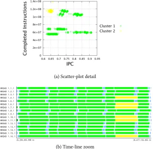
points with strong components, vertical and horizontal, where X-means has divided the isolated group. . . 46 4.3. X-means and DBSCAN algorithms comparison. Clusters time-line distribution 47 4.4. Cluster analysis of NPB BT class A Benchmark using clustering algorithm
over Completed Instructions and IPC. Due to the use of a restrictive Eps
value the structure is detected at fine grain . . . 48 4.5. A second cluster analysis of NPB BT class A Benchmark using the cluster
algorithm over Completed Instructions and IPC. Using higher value ofEps
produces a coarser grain detection, showing a SPMD structure . . . 49 4.6. Time-lines of different performance hardware counter metrics of WRF NMM
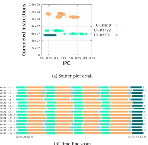
application executed with 64 tasks . . . 51 4.7. Cluster analysis with DBSCAN algorithm using Complete Instructions, L1
Data Cache Misses and L2 Data Cache Misses of WRF application executed executed with 64 MPI tasks . . . 53 4.8. Comparison of the clusters discovered on NPB BT class A Benchmark
presen-ted in Figure 4.5 and the main user functions of the application . . . 55 4.9. Comparison of the clusters discovered on HydroC and the main user
func-tions of the application . . . 57 4.10. Detailed plot of the clusters that represent the bi-modalupdateConservativeVars
of HydroC solver . . . 57 5.1. An example of alignment of the NAS BT Class A with 4 tasks. (a) shows the
cluster distributation in the time-line; (b) presents the proposed alignment computed by Kalign2 and depicted by ClustalX. . . 61 5.2. Results of the experiment bt_a_16_0057. Time-line (a), and alignment (b)
correspond to two iteration detail of the whole application . . . 64 5.3. Detected structure, sequences alignment and Cluster Sequence Score results
of bt_a_16_0150experiment. The figures corresponds to two iterations of
the whole application . . . 65 5.4. Detected structure, sequences alignment and Cluster Sequence Score results
ofwrf_16_0100experiment. The figures correspond to two iterations of the
whole application . . . 66 5.5. Detected structure, sequences alignment and Cluster Sequence Score results
ofwrf_16_0200experiment. The figures correspond to two iterations of the
whole application . . . 67 5.6. Detected structure, sequences alignment and Cluster Sequence Score results
ofwrf_16_0300experiment. The figures correspond to two iterations of the
whole application . . . 68 5.7. Detected structure, sequences alignment and Cluster Sequence Score results
offt_a_16_0090experiment. The figures correspond to a single iteration of
the whole application . . . 69
List of Figures
5.8. Detected structure, sequences alignment and Cluster Sequence Score results
oflu_a_16_0090experiment. The figures correspond to a single iteration of
the whole application . . . 70 6.1. Example of data set that require multiple Eps parameters. This data was
obtained from the Hydro solver executed with 128 tasks . . . 71 6.2. Complete aggregative refinement cluster analysis tree obtained from NPB
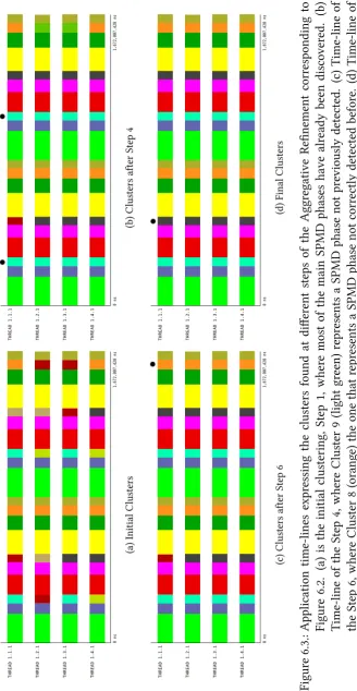
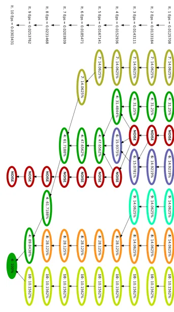
BT class A executed with 4 tasks. The empty nodes of the tree depict those clusters that are discarded because of poor SPMDiness and thus need to be merged. Filled nodes are those selected in the final partition of the data. In this case, due to the convergence, all selected nodes got 100% score. Each layer represents one step in the refinement loop. . . 76 6.3. Application time-lines expressing the clusters found at different steps of the
Aggregative Refinement corresponding to Figure 6.2. (a) is the initial clus-tering, Step 1, where most of the main SPMD phases have already been discovered. (b) Time-line of the Step 4, where Cluster 9 (light green) rep-resents a SPMD phase not previously detected. (c) Time-line of the Step 6, where Cluster 8 (orange) the one that represents a SPMD phase not correctly detected before. (d) Time-line of the final partition of the data, Step 7 in the tree, where Cluster 11 represents the last SPMD phase found. Dots on the top of the time-lines serve as guide to see the clusters mentioned. . . 77 6.4. sorted 4-distgraph obtained from the Socorro application. The red dots are
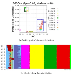
represent the distance to the 4th nearest neighbour for each point in the dataset. The blue line is the line defined by the points (0,max_k_dist) and (number_of_points/2, 0). We use it to compute the differentEpsvalues . 78 6.5. Computation structure detection of Hydro solver, using DBSCAN cluster
algorithm with the parametersM inP oints= 10andEps = 0.0200 . . . . 79 6.6. Computation structure detection of Hydro solver, using DBSCAN cluster
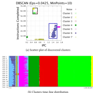
algorithm with the parametersM inP oints= 10andEps = 0.0425 . . . . 80 6.7. Computation structure detection of Hydro solver, using Aggregative Cluster
Refinement algorithm . . . 81 6.8. Detailed results of a DBSCAN cluster analysis of same phases present in
Figure 6.9 of WRF application. The parameters used were M inP oints= 4
andEps= 0.0470 . . . 82 6.9. Detailed results of a DBSCAN cluster analysis of WRF application. The
para-meters used wereM inP oints= 4andEps= 0.0896 . . . 83 6.10. Detailed results of the Cluster Aggregative Refinement of the same phases
of WRF application presented in Figures 6.9 and 6.8 . . . 84 6.11. Refinement tree depicting the formation pattern of Cluster 1 of VAC application 86 6.12. VAC Cluster 1 formation scatter plots. This plots correspond to the two
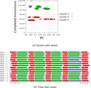
iterations of the refinement tree of Figure 6.11. . . 86 6.13. Cluster 1 distribution time-line of iterations iterations presented in Figure 6.11.
List of Figures
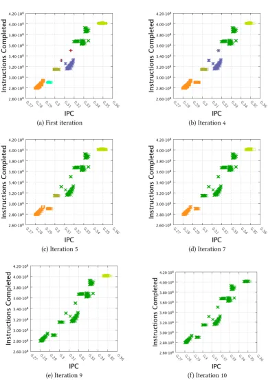
6.15. VAC Cluster 4 formation scatter plots. These plots correspond to the the first iteration of the algorithm and iterations observed in the refinement tree of Figure 6.14, where the Aggregative Cluster Algorithm merged two or more clusters. . . 89
6.16. Cluster 4 distribution time-line of iterations presented in Figure 6.15. The time-lines contain one repetition of the SPMD region detected . . . 90
6.17. Refinement tree depicting the formation pattern of Cluster 5 of VAC application 92
6.18. VAC Cluster 4 formation scatter plots. These plots correspond to the the two bottom levels of the refinement tree of Figure 6.17. . . 93
6.19. Cluster 5 distribution time-line of partitions presented in Figure 6.18. The time-lines contain one repetition of the SPMD region detected. . . 93
7.1. Example of a clustering of GAPgeofem application using the Aggregative Cluster Refinement with Instructions Completed and IPC. Upper left plot depicts the metrics used by the clustering algorithm. The rest of plots show the clusters found in terms of other pairs of metrics not used during the cluster analysis . . . 99
7.2. PEPC extrapolation errors for CPI breakdown model counters using different multiplexing strategies. Left column represents the relative error compar-ing the extrapolation and the actual value from non-multiplexed execution. Right column represents these errors weighted in terms of the relevance of each cluster with respect to the total cycles on the non-multiplexed run . . . 104
7.3. PEPC counters relevance with respect to Total Cycles counter . . . 105
7.4. TERA_TF extrapolation errors of counters listed in Table 7.1 model counters using different multiplexing schemes. . . 106
7.5. GAPgeofem extrapolation errors of counters listed in Table 7.1 model coun-ters using different multiplexing schemes. . . 107
7.6. GAPgeofem extrapolation errors of counters listed in Table 7.1 model coun-ters using different multiplexing schemes. . . 108
7.7. General CPI breakdown models of all applications presented in the paper. These models are a general view of the major categories, not using all 15 counters extrapolated to clarify its legibility. In all cases, they were com-puted the time-space multiplexing extrapolation method . . . 110
List of Figures
8.1. Simulation methodology cycle for a whole supercomputing application. Start-ing with a trace of a parallel application (step 1), we produce a sub-trace (or trace cut) containing information of just two iterations (step 2). A cluster analysis is applied to the information of the computation regions present on this reduced trace, and a set of representatives per cluster is selected (step 3), adding cluster information to the trace cut (step 4). The set of represent-atives is traced (step 5) and simulated using a low-level simulator to obtain the ratios on other possible processor configurations (step 6). Finally, using a full-system-scale simulator, we combine the communication information present in step 3 and the cluster instructions per cycle (IPC) ratios (step 6) to
predict the total runtime of the whole application (step 7). . . 112
8.2. Input data and the two stages of the phase detection analysis: periodic re-gion detection using the DWT and the iterative phase detection using the autocorrelation . . . 114
8.3. Execution time prediction error for Versatile Advection Code (VAC) and Weather Research Forecasting (WRF) parallel applications, for both self val-idation (a) and cross valval-idation (b) experiments. The figures show the error when estimating the execution time of two iterations of the application or the full application execution time with the measured real IPC and the IPC provided by MPsim. . . 123
8.4. Performance predictions of VAC using different cache sizes and network bandwidths . . . 126
8.5. Performance predictions of WRF using different cache sizes and network bandwidths . . . 127
9.1. PEPC refinement tree . . . 135
9.2. PEPC scatter plot of discovered clusters . . . 136
9.3. PEPC time-line distribution of clusters . . . 137
9.4. PEPC CPI breakdown model of the clusters found . . . 137
9.5. Clusters distribution time-line of nominal simulation, duration balancing simulation and the algorithmic improvement of PEPC application . . . 139
9.6. Results of the simulation when using PEPC in a different hardware . . . 141
9.7. PEPC clusters time-lines using 16384 MB/s network bandwidth and general purpose CPU 64 faster and accelerator 64 faster . . . 142
9.8. WRF scatter plot of discovered clusters . . . 143
9.9. WRF time-line distribution of clusters . . . 144
9.10. WRF refinement tree . . . 145
9.11. Clusters distribution time-line of nominal simulation, duration balancing simulation and the algorithmic improvement of WRF application . . . 148
9.12. Results of the simulation when using WRF in a different hardware . . . 150
9.13. WRF clusters time-lines using 16384 MB/s network bandwidth and general purpose CPU 64 faster and accelarator 64 faster . . . 151
9.14. GADGET scatter plot of discovered clusters . . . 152
List of Figures
9.16. GADGET refinement tree . . . 154
9.17. Clusters distribution time-line of nominal simulation, duration balancing simulation and the algorithmic improvement of GADGET application . . . . 156
9.18. Results of the simulation when using GADGET in a different hardware . . . 158
9.19. GADGET clusters time-lines using 16384 MB/s network bandwidth and gen-eral purpose CPU 64 faster and accelerator 64 faster . . . 159
9.20. SU3_AHiggs scatter plot of discovered clusters . . . 160
9.21. SU3_AHiggs time-line distribution of clusters . . . 162
9.22. Clusters distribution time-line of nominal simulation and the algorithmic improvement simulation of SU3_AHiggs application . . . 163
9.23. Results of the simulation when using SU3_AHiggs in a different hardware . 165 9.24. SU3_AHiggs clusters time-lines using 16384 MB/s network bandwidth and general purpose CPU 64 faster and accelerator 64 faster . . . 166
A.1. Scheme of the BSC Tools Parallel Performance Analysis Suite, depicting the different tools and their interaction . . . 179
A.2. Basic Paraver time-line view . . . 184
A.3. Detail of the Paraver Semantic Module showing the semantic functions re-garding thread states . . . 184
A.4. Communication and Event sections of the Paraver Filtering Module . . . 185
A.5. Paraver Histogram View . . . 186
A.6. Paraver process model . . . 187
A.7. Paraver and Dimemas resource model . . . 188
A.8. Paraver trace file structure . . . 188
A.9. Paraver trace header records definition . . . 190
A.10. Paraver state record specification . . . 191
A.11. Paraver event record specification . . . 191
A.12. Paraver communication record specification . . . 191
A.13. Dimemas communication diagrams . . . 193
A.14. Dimemas trace file structure . . . 195
A.15. First line of Dimemas trace header definition . . . 196
A.16. Paraver communicator definition record structure . . . 196
A.17. Dimemas CPU burst record definition . . . 197
A.18. Dimemas send operation record definition . . . 198
A.19. Dimemas receive operation record definition . . . 198
A.20. Dimemas collective operation record definition . . . 199
A.21. Dimemas event recod definition . . . 199
A.22. Dimemas offset record definition . . . 199
A.23. Dimemas system definition record structure . . . 201
A.24. Dimemas node definition record structure . . . 201
A.25. Dimemas mapping definition record structure . . . 202
A.26. Dimemas modules definition record structure . . . 202
A.27. Folding mechanisms scheme. Picture obtained from [6] . . . 205
A.28. Application of the folding mechanism to multiple performance counters . . . 206
List of Figures
A.29. Sequence of plots showing the program structure at different scenarios.
Pic-ture obtained from [7] . . . 207
B.1. UML class model of thelibClusteringlibrary . . . 210
B.2. UML class model of thelibTraceClusteringlibrary . . . 211
B.3. Bursts histogram produced bystatstool . . . 214
B.4. Output plots produced byBurstClusteringtool combining different metrics 218 B.5. A Paraver time-line and profile showing information related to a cluster ana-lysis . . . 219
B.6. Example of a refinement tree produced byBurstClusteringtool . . . 220
B.7. ClustalX sequence alignment window . . . 221
B.8. Clustering definition XML file structure . . . 222
B.9. Nodes to define the parameters extracted from a trace . . . 223
List of Tables
4.1. Clustering tool statistics for a set of applications used in the examples. The values regarding the NPB BT benchmark correspond to the execution with higher value ofEps . . . 50 4.2. Performance characterization of the 6 clusters that aggregate more than 90%
of the WRF application computing time of application analysis depicted in Figure 4.7 . . . 52 4.3. Code linking of the 6 main clusters of WRF application . . . 54 4.4. HydroC clusters/subroutines correspondence . . . 56 5.1. Summary of the different applications used in the experiments, as well as the
DBSCAN parameters used and the total number of clusters obtained . . . 62 7.1. List of all hardware counters used in the experiments to verify the
extrapol-ation technique . . . 102 7.2. Average value of weighted errors using different multiplexing schemes . . . 105 8.1. Reduction factors and quality evaluation of the different parts of the
Inform-ation Reduction step of WRF applicInform-ation . . . 118 8.2. Reduction factors and quality evaluation of the different parts of the
Inform-ation Reduction step of VAC applicInform-ation . . . 119 8.3. Baseline MPSim processor configuration . . . 120 8.4. Baseline Dimemas cluster configuration . . . 121 8.5. Real IPC vs. MPSim predicted IPC comparison in self validation experiment,
using two threads per core configuration . . . 122 8.6. WRF cross validation MPSim Ratios, comparing the IPC running two-threads
per core (CMP) and a single thread per core (ST) and the differences with the ratios in real configuration . . . 124 8.7. VAC cross validation MPSim Ratios and the differences with real ratios. In
this case, we just express the ratios and not the IPC on single thread and CMP configurations because of the higher number of representatives . . . . 124 9.1. List of all hardware counters used in the experiments . . . 130 9.2. Baseline Dimemas cluster configuration . . . 133 9.3. Cluster analysis results and factors of the speedup model defined in [8]
List of Tables
9.6. WRF clusters characterization . . . 146
9.7. WRF speedups of application improvement analyses . . . 147
9.8. GADGET clusters characterization . . . 152
9.9. GADGET speedups of application improvement analyses . . . 155
9.10. SU3_AHiggs clusters characterization . . . 160
9.11. SU3_AHiggs speed-ups according to potential cluster improvements . . . 162
A.1. Dimemas simulator parameters . . . 192
A.2. Dimemas collective communicationsM ODEL_[IN|OU T]_F ACT OR pos-sible values . . . 194
A.3. Dimemas collective communications options forSIZE_INandSIZE_OU T 195 A.4. Possible values ofglobal_op_idfield in a collective communication record of Dimemas . . . 200
B.1. Cluster algorithms included in thelibClusteringand their parameters . . 215
B.2. BurstClusteringtool parameters . . . 216
Part I.
1. Introduction
I
n this thesis we present novel techniques to characterize the performance of parallel ap-plications. The work is mainly focused on those parallel applications that run on high performance computing (HPC) systems. This chapter presents the motivation for the re-search and also introduces the Performance Analytics field, where this thesis is included. Finally, the chapter also contains a list of the contributions of the thesis as well as the book organization.1.1. Motivation
High Performance Computing and Supercomputing is the area of computing science that studies and develops the most powerful computers available. For example, the current #1 supercomputer in the world, according to the Top500.org list is Titan, a Cray supercomputer located at the Oak Ridge National Laboratory, Oak Ridge, Tennessee, United States. It has 560,640 processing cores (the smallest hardware unit capable of running one parallel process or thread) and its computation power is 17.590 PFlop/s. These figures are a good start to illus-trate the challenges in this scenario. To achieve this computing at this scale, supercomputers include a huge number of factors that affect their performance: processors, mathematical accelerators, more or less sophisticated interconnection networks, I/O systems.
In the same way, the applications that run on these kind of computers also have many factors that affect their performance. First, to take advantage of the huge amount of com-pute power available, the applications must be parallel. Essentially, a parallel application is an application where parts of its code can be executed at the same time, concurrently, producing partial results that later combine solve a given problem. In practice, the design and implementation of these parallel applications involve many elements that affect the per-formance: the sequential algorithms implemented, the distribution of the data it uses, the communications patterns of the different parallel parts, etc.
As a result, to achieve the maximum performance that a supercomputer offers, the theor-etical peakperformance of the hardware, the developer of a parallel application must take into account this huge number of factors to know and understand how its application be-have on it. This is the mission of the parallel performance analysis. In an application-centric approach, the performance analysis is a cyclic process consisting of observing the behaviour of the application so as to hypothesize the possible problems that affect its performance and finally translate these hypotheses to improvements in the application re-starting the cycle to validate them. Obviously, the less number of iterations of this cycle the less time wasted and also the less money spent.
1. Introduction
data, that will be later analysed to define the hypotheses and validate or discard them. At the scales defined previously (hundreds of thousands cores, petaflops of computing power) the performance data generation during an application execution is huge: up to millions of performance events per second. Thus, it is necessary to increase the power and intelligence of the performance tools available to deal with this such amount of performance data and then reduce the analysis iterations. That represents the main motivation of this thesis: how max-imize the knowledge of a parallel application performance when dealing with an enormous amount of performance data produced and also how to translate this knowledge to a per-formance tool that presents this information in an understandable way to the application analyst or developer.
1.2. Performance Analytics
Data Analyticsis the science of examining raw data with the purpose of drawing conclusions about that information. Performance Analytics is Data Analytics applied to performance analysis data. As presented in the next chapter, there are a relatively short list of works included in the different analysis toolkits under the umbrella of this term.
In general, current performance analysis toolkits offer a simplistic manipulations of the performance data. First-order statistics such as average or standard deviation are used to summarize the values of a given performance metric, hiding in some cases interesting facts available from the raw data. We consider that Performance Analytics techniques are neces-sary so here we introduce the techniques we propose in this field.
1.2.1. Cluster Analysis in the Parallel Performance Scenario
When analysing a parallel application, the amount of performance data that is generated is huge. Summarizing the information according to a given criteria is then a necessity. Ap-plication profiling is the common technique to summarize the performance information. A profile is a simple accounting of first order statistics over a set of metrics associated to an application-level abstraction, for example the application subroutines. The major drawback when using profiles is that the time-varying behaviour is hidden. For example, a given sub-routine could have different timings depending on duringo which phase of the application it is called. A profile will not make this distinction.
Considering the necessity to summarize the information in a more intelligent way that profiles do, we found cluster analysis to be better suited. As defined in [9], cluster analysis is the “unsupervised classification of patterns (observations, data items or feature vectors) into groups (clusters)”. The fact that is a classification and not an aggregation of the information is a key factor to overcome the intrinsic problem of the profiles, so the different trends in the data are not hidden.
For example, a classic use of cluster analysis is to reduce the amount of information gen-erated taken into advantage the repetitive patterns of parallel applications. In works such as [10, 11, 12], the authors exploited the structure of the Single Program Multiple Data (SPMD) paradigm that the vast majority parallel applications follow. In a SPMD
1.2. Performance Analytics
tion it is expected that all processes/tasks involved perform the same sequences of compu-tations/communications. In this context, cluster analysis is demonstrated to be effective to group those of processes/ tasks that behave similarly. Using a representative per cluster, the authors easily reduce the amount of performance data.
Our novel approach in the application of cluster analysis has a different target: determine the computational structure of the application. Instead of grouping the processes/tasks that behave similarly, we focus on the identification of the phases observed in the computation regions, i.e. those regions between communication primitives or calls to the parallel run-time, of a given parallel application. With our approach, we do not just take advantage of the SPMD pattern but also of the iterative applications design, for example in the wide variety of numerical methods used to solve equation systems. As a result, we obtain an small number of clusters characterize these repetitive structural computation phases, providing the developer/analyst an useful insight of applications computation behaviour.
Figure 1.1 compares these two different approaches. Picture 1.1a represents the different processes in a parallel application, where we have distinguished the computation (light grey) and communication (dark grey). Picture 1.1b represents the results of the approaches presen-ted in [10, 11, 12]: considering for example of the duration of the processes, they detect two different clusters that group two processes each. Picture 1.1c represents our approach, where we group the different computation parts that appear in the processes, obtaining three different clusters according to the duration of the computation regions.
1.2.2. Sequence analysis in Parallel Performance Scenario
In bioinformatics, sequence analysis [13] is the process of extracting useful information from biological sequences, such as DNA chains or proteins. Multiple Sequence Alignment (MSA) is a sequence analysis technique able to determine the similarities across two or more se-quences to define functional, structural or evolutionary relationships across them. These alignments are also used for non-biological sequences, such as those present in natural lan-guage [14] or in geographical studies [15].
Using the brief description of a parallel application provided previously, we can make this simple analogy: each activity (compute or communicate) that each process/task of the application performs in parallel to solve the desired problem could be seen as a DNA base or amino-acid element, so the sequence of activities would be the equivalent to a DNA chain or a protein. Using a MSA algorithm will tell us how similar are the different processes/tasks in terms of the sequences they perform.
That is especially relevant when the application follows the SPMD paradigm, because it is expected to have the same sequence of activities for all processes/tasks involved. Our contribution to the Performance Analytics in this aspect is a quality score that measures the
SPMDiness, i.e., how well it follows the SPMD paradigm of the structure of a given parallel application.
1. Introduction
Task 1
Task 3
Task 4 Task 2
(a) Original sequence of computation/communication to analyse
Cluster 1 = {Task 1, Task 3} / Cluster 2 = {Task 2, Task 4} Cluster 1
Cluster 2
(b) Cluster analysis to detect tasks/threads with similar behaviour
Cluster 1 Cluster 2 Cluster 3 Task 1
Task 2
Task 3
Task 4
(c) Cluster analysis to detect computation regions with similar behaviour
Figure 1.1.: Comparison of cluster analysis targets
1.3. Contributions
1.3. Contributions
As a summary of this chapter, we want to emphasize that this thesis introduces two new techniques in the Performance Analytics field, with the target of improving the knowledge of parallel application performance. More precisely, we present cluster analysis for detecting the computational structure and the application of sequence analysis to evaluate the SPMD structure.
The contributions of this thesis can be classified into two main categories. The first one corresponds to the technical contributions to create and validate the new techniques. The second category corresponds to the concrete examples ofapplyingthe techniques to different areas of performance analysis.
1.3.1. Technical Contributions
Demonstration of the suitability of density-based cluster algorithms to detect computation structure
We demonstrate the suitability of density-based cluster algorithms, specifically DBSCAN, when characterizing the computation structure of parallel applications. We show that this kind of algorithm surpasses the clustering algorithms based on K-Means when grouping performance hardware counters (HWC) data, and work more effectively than hierarchical clustering algorithms because they do not require an user interaction.
Design and validation of a cluster quality score for SPMD computation patterns detection
To fulfil the necessity of quantitative evaluate the computation structure a given application, we introduced the Cluster Sequence Score. This score is calculate by means of a Multiple Sequence Alignment (MSA) algorithm to evaluate theSPMDiness, i.e. how well the different sequences of actions in a parallel application follow the SPMD paradigm.
Design and validation of a new cluster algorithm to refine the computation structure detection
1. Introduction
1.3.2. Examples of applications of the techniques presented
Design and validation of a performance data extrapolation methodology using structure detection
In some cases, we need to execute an application several times to obtain different metrics that cannot be read simultaneously, for example when using processor hardware counters. We present the design and validation of a performance data extrapolation methodology that solves this problem by multiplexing the data acquisition along the (repetitive) application phases, and then extrapolates the average values per phase of a wide number of performance metrics.
Design and validation of a methodology to minimize the volume of the input data in a multi-level simulator of parallel applications
Detailed simulations of large scale message-passing parallel applications are extremely time consuming and resource intensive. We present the design and validation of a methodology where the structure detection is combined with signal processing techniques capable of re-ducing the volume of simulated data by hundreds to thousands orders of magnitude. This reduction makes possible detailed software performance analysis and accurate predictions in reasonable time.
Parallel applications what-if studies
Using the structure detection, we present a set of what-if studies of four production-class parallel applications. To perform these studies, we use the structure detection combined with an application level simulator. As a result, we show how what will be gained by im-proving the applications, without the need to actually changing the code, and also what will be the expected performance when porting the applications to different hardware, without requiring the real machines.
1.4. Dissertation Organization
The rest of this book is organized as follows. The Chapter 2 contains a discussion of the previous work in the parallel performance field, including the major work in the Perform-ance Analytics field. Chapter 3 is an introduction to cluster analysis algorithms and multiple sequence alignment algorithms, important to understand the Performance Analytics tech-niques developed. In Chapter 4, we demonstrate the suitability of density-based clustering algorithms to effectively determine the computation structure of message-passing parallel applications. In Chapter 5, we present the Cluster Sequence Score, a score to evaluate the SPMD structure of a parallel application. In Chapter 6, we present Aggregative Cluster Re-finement, a density-based clustering algorithm that detects the computation structure at fine grain, without user interaction. In Chapter 7, we present a methodology to extrapolate per-formance data using a structure detection to maximize the information extracted in a single
1.5. Publications
application run. In Chapter 8, we use the computation structure obtained combined with sig-nal processing techniques to minimize the input data in a multi-level simulator. In Chapter 9, we present an analysis of four parallel applications by using the Aggregative Cluster Re-finement. In Chapter 10, we discuss the contributions presented as a whole, describing the research and development opportunities that it offers to the community. In Appendix A, we detail the BSC-Tools suite, the performance analysis toolkit used to developed and valid-ate the work presented in previous chapters. Appendix B contains the software engineering foundations of the CluteringSuitepackage, the software piece included in the BSC Tools suite that contains the implementation of the ideas and methodologies presented.
1.5. Publications
[16] J. Gonzalez, J. Gimenez, and J. Labarta. Automatic Detection of Parallel Applications Computation Phases. In IPDPS ’09: Proceedings of the 23rd IEEE International Parallel and Distributed Processing Symposium, Rome, Italy, May 2009
[17] J. Gonzalez, J. Gimenez, and J. Labarta.Automatic Evaluation of the Compu-tation Structure of Parallel Applications. InPDCAT ’09: Proceedings of the 10th International Conference on Parallel and Distributed Computing, Applications and
Technologies, Hiroshima, Japan, December 2009
[18] J. Gonzalez, J. Gimenez, and J. Labarta. Performance Data Extrapolation in Parallel Codes. In ICPADS ’10: Proceedings of the 16th International Conference on Parallel and Distributed Systems, Shanghai, China, December 2010
[19] J. Gonzalez, J. Gimenez, M. Casas, M. Moreto, A. Ramirez, J. Labarta, and M. Valero.Simulating Whole Supercomputer Applications.IEEE Micro,31:32– 45, 2011
2. The Parallel Performance Analysis
Field
P
arallel performance analysis is a process that starts by extracting the raw performancedata that will be later analysed to determine the potential problems of the application. In this context, we want to distinguish three important aspects that compose the whole process: when the analysis is done; the data used to characterize the performance; and finally, the different methods, techniques and applications to analyse this data to draw the conclusions.2.1. Analysis Placement
The analysis placement refers to when the analysis is going to take place. Here we distin-guish betweenon-lineanalyses, where the measurements and hypothesis are done during the application execution, and thepost-mortemwhere the information is collected and stored to be later analysed when application finishes. We do not want discuss the detailed implica-tions of the analysis location in the performance analysis process because, in most cases, the techniques or methods are applicable to both scenarios.
2.2. The Performance Data
To understand the behaviour of a parallel application on a given machine, we need to meas-ure different elements that reflect its performance. The most simple and recurrent element measured is the application execution time. Undoubtedly, the execution time is a good in-dicator of the application performance, and in most cases is the objective value to minimize. In the performance analysis scenario, it is also common to use time, but a finer grain, for example measuring the time spent on each application subroutine. To perform these measurements, we can make use of the timing mechanisms provided by the operating system (OS), for example the programmable clock interrupts. In addition, this example points to a second performance metric: the application code location. Location information is required to relate the metrics to the application source code. This location can be a single position where the measurement is taken, accessed via the Program Counter (PC) of the CPU, or the
call path, that includes the list of active subroutines in the application, accessed unwinding the call stack, for example usinglibunwind[21].
2. The Parallel Performance Analysis Field
all modern processors, and count micro-architectural events such as the total cycles elapsed or the number of instructions executed. Hardware vendors provide the hardware and soft-ware interface to access these counters, but the PAPI [22] library, a homogeneous application programming interface to access the counters in most of the hardware, is the most common way to read them. More recently, due to the need to better understand new hardware, we can also find performance hardware counters in other components beyond CPUs, such as the Infiniband network hardware [23] or the Nvidia CUDA GPUs [24]. In both cases, the counters are also available via PAPI.
The metrics regarding the parallel programming model are varied, as well as the mechan-isms to access them. For example, in the message-passing applications, the ones we analyse in this thesis, it is normal to gather the number of messages sent or received, the size of these messages, etc. In this case, if the application uses MPI, we have available the MPI profiling interface (PMPI) [25] to intercept the MPI calls and extract these values. In some other cases, access to the run-time of the programming models requires more sophisticated mechanisms, as detailed in next section when talking about instrumentation.
Apart from this list, there are a variety of metrics to evaluate specific performance ele-ments (I/O, power consumption, etc.). It is not the aim of this section to present every performance metric available, but those commonly available in most performance toolkits.
2.2.1. Data Acquisition
We can distinguish two different methods to obtain performance data: samplingthe applic-ation orinstrumentingit.
Sampling consists of taking measures of the application status at regular intervals or when a certain condition happens. In this way, the measurements are taken independently from the application behaviour. Usually, for each sample, the information collected is the application location plus a set of quantitative metrics, such as the performance counters. Using sampling, the specific metrics of the programming model used are difficult to access.
When using sampling, the precision of the samples is directly related to the intrusiveness of the method: higher sample rates imply more precision but more overhead and perturba-tion of the results.
Application instrumentation consists of adding additional instructions or probes to the regular application code to capture those events and metrics that provide insight of the ap-plication behaviour, essentially entry or exit to apap-plication subroutines or the programming model run-time. As opposed to sampling, it is the application implementation that drives the data acquisition. In this way, the location is implicit, but sometimes the full call path is also recorded. As in sampling, other metrics such as the performance counters metrics are recorded when an event is captured.
The mechanisms to instrument an application are many. Instrumentation can be done manually by modifying the source code but also using more sophisticated methods: code to code translation with instrumentation injection, such as the OPARI [26] translator for OpenMP; rewriting application binaries as DynInst [27]; or dynamically modifying the ap-plication at run-time, also offered by DynInst and Intel’s PIN [28]. It is also possible to use
2.2. The Performance Data
the profiling interfaces of some libraries, such as PMPI, that provide access to those metrics of the programming model not available when using sampling.
2.2.2. Emitted Data
Before starting the actual analyses, there is classical dichotomy describing how the inform-ation is emitted and therefore stored: applicinform-ation profiles or event traces. The way the information is stored partially determines the kind of analyses available.
Application Profiles
An application profile is a summarization of a metric, or a set of metrics, that characterize an application-level abstraction. A typical example of a flat profile is the number of calls and the time spent in each application subroutine. In the process of summarization, the temporal component information regarding when the data was collected is lost.
gprof [29] is the classic tool for profiling sequential codes. This tool relies on compiler
assisted instrumentation to define the bounds of the application subroutines and the POSIX timers and signalling to take the samples. It generates partial call graph profiles, more de-tailed profiles that express the caller-callee relationships across the application subroutines.
OpenSpeedshop [30] and the HPCTOOLKIT [31] extendgprof capabilities focusing on parallel applications. Both are able to manage the information generated by all tasks/threads involved in a parallel application, so as to present a single profile. In addition, they provide the ability to profile not only application subroutines but also basic blocks of code, or even single individual source code lines.
gprof, OpenSpeedshop and HPCTOOLKIT heavily rely on sampling mechanisms to
per-form the data acquisition. On the other hand, TAU [32] from the University of Oregon provides a profiling toolkit based on instrumentation mechanisms to allow the user a fine control on what is going to by profiled, including MPI run-time accesses and performance hardware counters. TAU also gathers phase profiles, partial profiles extracted at different
states of the application execution. We can find in [33] a study of these different states or phases, into the IPS-2 analysis toolkit. In the case of TAU, the states are defined by the user and can be understood as the logical steps in the application evolution, for example the dif-ferent time-steps in a weather forecast simulation. The phase profiles provide an approach to observe the time-varying behaviour of an application.
The Scalasca toolkit [34] also offers the collection of regular profiles with metrics from MPI, OpenMP and hardware counters using instrumentation. In this toolkit ecosystem we also find an interesting effort gatheringtime-series call-path profiles[35], call-graph oriented version of the previously mentioned phase profiles.
Event Traces
2. The Parallel Performance Analysis Field
the parallel libraries used, values of the hardware counters or the call-path that lead to the point of interest. Tipically, the generation of event traces relies on instrumentation packages to define the points of interest, but we can also find sample traces. Event traces offer a highly detailed view of the performance, at the cost of high storage space requirements. They are especially interesting to analyse the time-varying behaviour of the application, information that is totally lost when using profiles.
In general, almost all parallel performance analysis toolkits offer the extraction of event traces as the base to the further analysis. For example the BSC Tools package, the toolkit used in this thesis, is based on Paraver trace [36]. This trace is a structured text file whose main characteristic is that it is semantic free: the events contained are essentially time-stamped key/value pairs. A complementary (optional) file is the responsible for linking the semantics to the tuples contained on the trace file. A detailed description of the Paraver trace is available in Appendix A.
Recently, as a part of the Score-P initiative [37], the analysis toolkits Scalasca, Vampir [38], Periscope and TAU decided to adopt the Open Trace Format version 2 (OTF2) [39], the second generation of the Open Trace Format [40]. OTF2 is structured in a collection of multiple binary files accessible via an API. The main concern in the design of this trace is the scalability: the trace format definition includes a series of encoding techniques to reduce its size [41], and the access API uses techniques to reduce the memory footprint.
As mentioned before, there are also some efforts to producesample traces. As opposed to the regular traces whose events are associated to instrumentation points, sample traces con-tain a series of time-stamped samples taken regularly during the execution. The information in each sample mainly includes the call-path, to correlate to application source code, and performance metrics, such as the hardware counters. We find an early approach to the gen-eration of sample traces inside the Sun Studio Performance Tools (now Oracle Studio) [42]. Recently, the HPCTOOLKIT and the BSC Tools also added sample traces on their toolkit ecosystems, [3] and [6] respectively. It is interesting to highlight that the addition of samples to the Paraver trace described in [6] did not imply any modification of the trace format.
2.3. Analysing the Performance Data
In a post-mortem scenario, once the data has been collected, the analysis step consists of exploring the information gathered, manually or assisted, to detect patterns or trends that reflect anomalies or performance losses in the application behaviour and correlate them with the possible causes.
At this point, we distinguish between two different elements of the analysis itself. The first is how the information is presented to the analyst to make the analysis process under-standable and manageable. The second is the collection of Performance Analytics techniques available, i.e. the different techniques developed to automate the processing of the raw data so as to detect anomalies and correlations.
2.3. Analysing the Performance Data
2.3.1. Data Presentation
Data presentation is a key element of the analysis process. The way the information is offered to the analyst defines, to some extent, the possible observations and hypotheses they could make about the performance achieved by the application. Undoubtedly, the way data is emitted imposes a series of restrictions or opportunities on its presentation.
Again, due to the (potentially) huge volume of data generated, this step may include a series of transformations or manipulations to present the information in a clear and concise manner.
Presentation of Profiles
Application profiles are an explicit example of this data manipulation per se. The different measurements taken during the execution are accounted in first order statistics such the sum or the average at the selected application-level abstraction (subroutines, application phases, etc.). Using profiles, the exploration for the unusual situations can be done easily. For example sorting total time spent in the different subroutines will point us where are the hotspots. The weak point of profiles is that the aggregation hides the potential variability across the instances accounted, but for a initial look of the performance, profiles are a good choice.
In general, profiles are presented as human-readable plain text files. The text is indented to categorize the elements accounted more easily and they are sorted with respect to one of the metrics used to focus the analysis. In Figure 2.1 we can see a flat profile produced bygprof. It contains the different metrics calculated for each subroutine, right-most column, sorted by the percentage of total application time spent each one represent, left-most column. The rest of the metrics include the exclusive/inclusive times (time inside the subroutine excluding or including the calls it makes) and number of calls. The call-graph profile in Figure 2.2 contains similar metrics, but the right-most column presents the caller-callee relationship using the indentation. These call-graph profiles generated bygprofcan also be visualized in a interactive GUI, using a tree representation, with the IBM’s Xprofiler [43].
In contrast to the simple plain-text document, we find tools such as thehpcviewer[44], an evolution of the HPCVIEW [45], which is the profile visualization tool of the HPCTOOLKIT.
Thehpcvieweris a GUI that offers a clean presentation of the different metrics gathered in
the HPCTOOLKIT profiles, with the ability to link the metrics with the source code, shown in Figure 2.3, or present the metrics using charts for a better comprehension, shown in Figure 2.4.
ParaProf [46], the profile analysis tool of the TAU package, offers similar functionality to
the hpcviewer, in the areas of source code correlation and the generation of different chart
2. The Parallel Performance Analysis Field
Each sample counts as 0.01 seconds.
% cumulative self self total time seconds seconds calls ms/call ms/call name 33.34 0.02 0.02 7208 0.00 0.00 open 16.67 0.03 0.01 244 0.04 0.12 offtime 16.67 0.04 0.01 8 1.25 1.25 memccpy 16.67 0.05 0.01 7 1.43 1.43 write
16.67 0.06 0.01 mcount
0.00 0.06 0.00 236 0.00 0.00 tzset 0.00 0.06 0.00 192 0.00 0.00 tolower 0.00 0.06 0.00 47 0.00 0.00 strlen 0.00 0.06 0.00 45 0.00 0.00 strchr 0.00 0.06 0.00 1 0.00 50.00 main 0.00 0.06 0.00 1 0.00 0.00 memcpy 0.00 0.06 0.00 1 0.00 10.11 print 0.00 0.06 0.00 1 0.00 0.00 profil 0.00 0.06 0.00 1 0.00 50.00 report
Figure 2.1.: Example of flat profile produced bygprof. Extracted from thegprofmanual[1]
granularity: each sample hit covers 2 byte(s) for 20.00% of 0.05 seconds
index % time self children called name
<spontaneous> [1] 100.0 0.00 0.05 start [1]
0.00 0.05 1/1 main [2] 0.00 0.00 1/2 on_exit [28] 0.00 0.00 1/1 exit [59]
---0.00 0.05 1/1 start [1] [2] 100.0 0.00 0.05 1 main [2]
0.00 0.05 1/1 report [3]
---0.00 0.05 1/1 main [2] [3] 100.0 0.00 0.05 1 report [3]
0.00 0.03 8/8 timelocal [6] 0.00 0.01 1/1 print [9] 0.00 0.01 9/9 fgets [12]
0.00 0.00 12/34 strncmp <cycle 1> [40] 0.00 0.00 8/8 lookup [20]
0.00 0.00 1/1 fopen [21] 0.00 0.00 8/8 chewtime [24] 0.00 0.00 8/16 skipspace [44]
---[4] 59.8 0.01 0.02 8+472 <cycle 2 as a whole> [4] 0.01 0.02 244+260 offtime <cycle 2> [7] 0.00 0.00 236+1 tzset <cycle 2> [26]
---Figure 2.2.: Example of call-graph profile produced by gprof. Extracted from the gprof
manual[1]
2.3. Analysing the Performance Data
2. The Parallel Performance Analysis Field
Figure 2.4.: Example of scatter plot of Completed Instructions counter produced by HPCTOOLKIT’shpcviewer. Image obtained from HPCTOOLKIT manual[2]
2.3. Analysing the Performance Data
three different executions of the same application with different configurations.
Figure 2.5.: TAU’s ParaProf thread hotspots profile window
Finally, Scalasca’s CUBE [48] visualizer has an original way to visualize and interact with profiles. The main display of this GUI is divided in three parts (see Figure 2.7). The left part shows the different metrics gathered; the central part is the code location; and the right part shows the system location, i.e. the accounting of each metric in the physical hardware. Thanks to the colouring, the user can see quickly the severity of a given metric, viz. low, regular or high values. In the example shown, the metric selected was the time spent in ’Point-to-Point’ message-passing primitives (left column), which has a relatively low severity (yellow). This metric appears in several subroutines in the call-path tree (central column) with medium severity, having the selected one, hsmoc, a medium high value in the visible range. Finally, the value of “Point-to-Point” time spent in thehsmocsubroutine is distributed uniformly in all the system (right column), with relatively high severity.
Event Traces Presentation
As opposed to profiles, event traces have greater potential to detect elements at finer granu-larity, as they keep track of all the actions performed by the analysed application, including the spatial and temporal distribution of them. On the other hand, traces require more effort both in the manipulation and the exploration to detect the anomalies and correlate them to the root causes.
2. The Parallel Performance Analysis Field
Figure 2.6.: TAU’s ParaProf thread profiles comparison
2.3. Analysing the Performance Data
2. The Parallel Performance Analysis Field
where the information available in the trace is organized in a bi-dimensional plot, applica-tions abstracapplica-tions such as tasks or threads versus time, and coloured according to a metric.
Figure 2.8 contains an example of the Vampir master time-line, presenting an OTF trace. In this case, the Y axis represents the processes of a message-passing application, and the colouring indicates the subroutine executed. We can also observe black lines that represent the point-to-point messages passed between the different processes. In the top left part of the window we can see a general view of the whole trace, being the main-time line just a zoom of the central part.
Figure 2.8.: Master time-line of VAMPIR trace analyzer
Figure 2.9 contains the equivalent window of the hpctraceviewer. In this case, since sample trace it presents does not have information regarding the point-to-point communica-tions, the time-line does not include communication lines. On the other hand, in the bottom part of the window it present the depth of the call-path obtained on each sample of the trace. Finally, in Figure 2.10 we can see an example of Paraver time-line. In this example, the metric selected was the Instructions per Cycle (IPC), derived from the Completed Instruc-tions and Total Cycles hardware counters present on the trace. The colouring is a gradient from light green (low IPC) to dark blue (high IPC). Paraver traces also contain point-to-point messages information, and these are depicted as yellow lines in the time-line.
Even though the time-line representation is useful to explore the time distribution of a raw (or derived) metrics at different levels of granularity using zooming, there are limitations to this representation: first, current screen resolutions limit the amount of data that can be
2.3. Analysing the Performance Data
Figure 2.9.:hpctraceviewerinterface. Picture obtained from [3]
2. The Parallel Performance Analysis Field
presented; second, there is a biological limit to distinguish differences the colour hue. These limitations imply that the representation requires a big effort in processing the input data to render how each pixel of the bitmap is filled. For example, a single pixel of the screen may represent more than one object or a wide range of time, so an algorithm is required to decide how depict this the actual value. For example, non-linear renderings of the data ranges are used to clarify the representation of the different values presented.
(a) Communication statistics summary
(b) Subroutine profiling summary
Figure 2.11.: Vampir summary windows
To overcome these constraints, the trace analysers, mainly Vampir and Paraver, also in-clude a set of features to manipulate the information available in the event trace. In the case
2.3. Analysing the Performance Data
of Vampir, it offers a battery of predefined summaries that include the generation of com-munications profiles, Figure 2.11a, and also flat-profiles, Figure 2.11b. Paraver also includes a profiling view, but extends the regular summarization with the ability to freely combine different metrics available, to detect the possible correlations across them. For example, in Figure 2.12a, there is a window of a profile showing the average IPC obtained by each ap-plication subroutine (columns) for each apap-plication thread (rows). In Figure 2.12b, we can see a complex histogram where the X axis represents ranges of values of the IPC, the Y axis represents the different threads of the application and the colouring expresses the number of L2 data cache misses (using the green-to-blue gradient). Even these two tools differ in the features to combine performance metrics, both are able to compute a wide range of statistics, similar to profiles: sums, averages, standard deviations, etc.
(a) Profile Metrics window (showing average IPC per subroutine per application thread)
(b) Metrics Combination Histogram (showing Main Memory Ac-cesses per IPC range per application task)