“Essays on Open Economy, Inflation, and Labour
Markets”
Alessia Campolmi
Universitat Pompeu Fabra
Department of Economics and Business
Director: Prof. Jordi Gal´ı
Corresponding Addresses: Alessia Campolmi
Central European University
Economics Department N´ador utca, 9
H-1054 Budapest (Hungary)
Phone: (+36) 1 3273000 (int.2369)
Magyar Nemzeti Bank
Research Division Szabads´ag t´er 8-9
H-1051 Budapest (Hungary)
Table of Contents ii
Acknowledgements iv
Introduction v
1 Which inflation to target? A small open economy with sticky wages 1
1.1 Introduction . . . 1
1.2 Related literature . . . 4
1.3 The model . . . 7
1.3.1 Households . . . 7
1.3.2 Firms . . . 13
1.3.3 Equilibrium Conditions . . . 14
1.3.4 The New Keynesian Phillips Curve (NKPC) . . . 16
1.4 Welfare function . . . 18
1.5 Optimal MP . . . 20
1.6 Interest rate rules . . . 22
1.6.1 Baseline calibration . . . 23
1.6.2 Performance of different monetary policy rules . . . 24
1.6.3 Main robustness checks . . . 25
1.6.4 Other checks . . . 28
1.7 Conclusions . . . 29
2 Labor Market Institutions and Inflation Volatility in the Euro Area 31 2.1 Introduction . . . 31
2.2 Stylized Facts . . . 33
2.3 A Model for A Currency Area with Labor Market Frictions . . . 36
2.3.1 Households in the Domestic and Foreign Country . . . 36
2.3.2 The Production Sector In the Domestic and the Foreign Region 39 2.3.3 The Monetary Policy Rule in the Currency Area . . . 45
2.3.4 Equilibrium Conditions . . . 45
2.3.5 Calibration . . . 46
2.4 Quantitative Properties of the Model . . . 47
2.4.1 Matching the Data . . . 51
2.4.2 The Impact of Employment Protection . . . 52
2.5 Conclusions . . . 54
3 Oil price shocks: Demand vs Supply in a two-country model 61 3.1 Introduction . . . 61
3.2 Related literature . . . 66
3.3 Stylized facts . . . 69
3.4 The model . . . 72
3.4.1 Household problem . . . 73
3.4.2 Firm problem - Final goods sector . . . 75
3.4.3 Firm problem - Intermediate goods sector . . . 76
3.4.4 Equilibrium conditions . . . 78
3.4.5 Flexible prices and wages . . . 80
3.4.6 Sticky prices and wages . . . 82
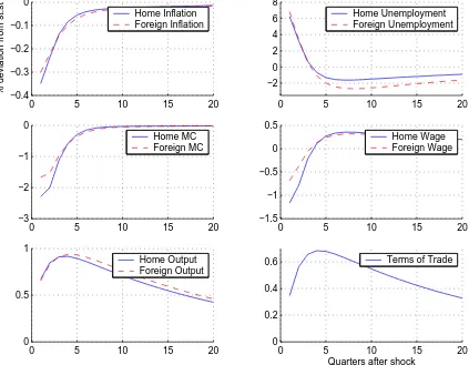
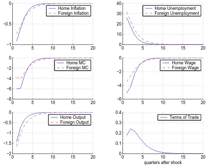
3.5 Demand vs Supply Shock: Impulse Response Analysis . . . 84
3.5.1 Baseline Calibration . . . 84
3.5.2 Demand vs Supply Shock . . . 85
3.6 Conclusions . . . 88
A Chapter 1 97 A.1 Derivation of mcct . . . 97
A.2 Derivation of the loss function . . . 98
A.2.1 Step 1: Derivation ofWt−W . . . 98
A.2.2 Step 2: Derivation ofEh[nbt(h)] and Eh[bn2t(h)] . . . 100
A.2.3 Step 3: Derivation ofWt−Wtn . . . 100
A.2.4 Step 4: Derivation ofV arh[wt(h)] . . . 102
A.2.5 Final expression . . . 103
A.3 System of equations fully characterizing the model . . . 104
B Chapter 3 106 B.1 Derivation of mcct . . . 106
To my supervisor Jordi Gal´ı, I own the first acknowledgment. For his questions, which always helped me very much, especially at the beginning of a new project, in the understanding of where to go, what to look for and how to look for it. Many times I had the impression that my understanding of my own ideas was improved after a talk with him! And for the constance with which he has always stimulated me in the search for further improvements of my work.
I’m also very thankful to Michael Reiter and Ester Faia for many useful discussions which have considerably improved the quality of my research. And also to Jaume Ventura, Thijs van Rens and all seminar participants at UPF.
A special thank to Stefano Gnocchi, Chiara Forlati and Harald Fadinger, not for the uncountable number of useful discussions, but for their friendship!
The usual disclaimer applies.
Finally, I want to dedicate this thesis to my parents, for having always believed in me in those years (and especially when I didn’t, which may happen during the life of a PhD student!), and for their love.
Barcelona, November 2007 Alessia Campolmi
In these last years there has been an increasing literature developing DSGE Open
Economy Models with market imperfections and nominal rigidities. It is the so called
”New Open Economy Macroeconomics”. Up to now within this class of models (and differently from what it is happening in New Keynesian closed economy models)
relatively little attention has been devoted to the labour markets. The first two
chapters provide two cases where relaxing the assumptions of perfect competition and no frictions in the labour market is important for the question addressed. In the first
chapter monopolistic competition in the labour market and nominal wage rigidities
are introduced in an otherwise standard small open economy model. Within this framework we address the question of whether the presence of sticky wages provides
a rational for Consumer Price Inflation targeting in the model. In the second chapter
we introduce matching and searching frictions in the labour market and relate different labour market structures across European countries with differences in the volatility
of inflation across the same countries. In the last chapter we use a two-country model
with oil in the production function and price and wage rigidities to relate movements in wage and price inflation, real wages and GDP growth rate to oil price changes.
In particular, in chapter one the focus is on which measure of inflation should
be used by the monetary authority as a target variable in a open economy context. Indeed, while there is common agreement on price inflation stabilization being one
of the objectives of monetary policy, in an open economy two alternative measures
of inflation coexist: domestic inflation and consumer price inflation (CPI inflation).
Which one of the two should be the target variable? Most of the literature suggests that the monetary authority should try to stabilize domestic inflation. This is in
sharp contrast with the practice of many inflation-targeting central banks which are
using CPI inflation as a target variable. Using a small open economy model we show that CPI inflation targeting can be rationalized by the presence of sticky wages.
After deriving the welfare function from a second order approximation of the utility
function, we compute the optimal monetary policy under commitment and use it as a benchmark to compare the performance of different monetary policy rules. The
rule performing best is the one targeting wage inflation and CPI inflation. Moreover,
the performance of this rule is close to that of the optimal monetary policy with commitment.
In chapter two1 the focus is on the Euro area. In particular, we start from the
observation that despite having had the same currency for many years, EMU countries still have quite different inflation dynamics. We explore one possible reason: country
specific labor market institutions, giving rise to different inflation volatilities. When
unemployment insurance schemes differ, as they do in EMU, reservation wages react differently in each country to area-wide shocks. This implies that real marginal costs
and inflation also react differently. We report evidence for EMU countries supporting
the existence of a cross-country link over the cycle between labor market structures
on the one side and real wages, real marginal costs and inflation on the other. We then build a DSGE model that replicates the data evidence.
Finally, chapter three focuses on the current increase in oil price. From the last
quarter of 2001 to the third quarter of 2005 the real price of oil increased by 103%. Such an increase is comparable to the one experienced during the oil shock of 1973.
At the same time, the behaviour of real GDP growth, Consumer Price inflation (CPI
inflation), GDP Deflator inflation, real wages and wage inflation in the U.S in the 1970s was very different from the one exhibited in the 2000s. What can explain such
a difference? Within a two-country framework where oil is used in production, two
kinds of shocks are analyzed: (a) a reduction in oil supply, (b) a persistent increase in foreign productivity (as proxy for the experience of non-OECD countries in the last
years). It is shown that, while the 1970s are consistent with a supply shock, the shock
to foreign productivity generates dynamics close to the one observed in the 2000s.
Which inflation to target? A small
open economy with sticky wages
1.1
Introduction
The purpose of the present paper is to analyse which measure of inflation should
be chosen as target variable in an open economy framework. In a closed economy
context there is common agreement on price inflation stabilization being one of the
main objectives of monetary policy. From the ad-hoc interest rate rule proposed by
Taylor (1993), to the more recent New Keynesian literature deriving optimal monetary
policy rules from the minimization of a microfounded loss function, the monetary
instrument has to be chosen in order to match a given inflation target (among with
other targets). However, in an open economy context two alternative measures of
inflation coexist: domestic inflation and consumer price inflation (CPI inflation). For
most of the OECD countries those two variables display different dynamics therefore,
a relevant question is which one of these two should be used by the monetary authority
as target variable. This is the question addressed in the paper.
With this purpose in mind, we develop a small open economy model similar to
the one used by Gal´ı and Monacelli (2005). The main difference with respect to that
model is the introduction of sticky wages. Under this assumption the volatility of
CPI inflation and the impossibility for some workers to adjust their wages in order
to keep their markups at the desired level makes the stabilization of CPI relevant
in this context. In particular, the assumption on wages has two main consequences:
first, given the presence of wage rigidities, strict inflation targeting will no longer be
optimal (as Erceg, Henderson and Levin (2000) show in a closed economy setup);
second, fluctuations in CPI inflation will induce undesired fluctuations in wage mark
ups and, therefore, in firms’ marginal costs and domestic inflation.
The main result of the paper is that, reacting to changes in CPI inflation instead
of focusing on targeting domestic inflation, the monetary authority will obtain better
results in terms of stabilizing wage inflation and output gap. This makes it desirable
to stabilize CPI inflation rather than domestic inflation. The importance of this
result is that, differently from the existing open economy literature, it is in line with
the practice of inflation-targeting central banks. Indeed, from an operational point
of view, there seems to be an unanimous consensus among central banks on CPI
inflation being the correct target. In particular, as stressed by Bernanke and Mishkin
(1997), starting from 1990 the following countries have adopted an explicit target
to CPI inflation: Australia, Canada, Finland, Israel, New Zealand, Spain, Sweden,
UK. To this list we can add more recently Norway and Hungary. In the EMU,
the European Central Bank has the objective to stabilize the Harmonized Index of
Consumer Prices (HCPI) below 2%. In contrast, from a theoretical point of view,
most of the literature suggests that the monetary authority should choose domestic
inflation as target variable for inflation1. Hence, the contribution of the paper is to
show that the introduction of sticky wages may help reconcile the workhorse model
for monetary policy analysis in an open economy with the practice of many monetary
authorities.
Regarding the assumptions on which the results of the paper are built, there
is strong empirical evidence of wage rigidity in the economy2. As underlined by
Christiano, Eichenbaum and Evans (2005) and by Smets and Wouters (2003), the
introduction of wage rigidity is a crucial assumption in order to improve the ability
of the New-Keynesian models to match the data. Consequently, there is empirical
evidence in favour of the importance of modelling also wage rigidity in order to obtain
more reliable dynamics.
Solving the model under the assumption of sticky wages and looking at the Phillips
Curve and the wage inflation equation a clear relation between domestic, CPI and
wage inflation emerges. In particular, changes in the CPI inflation induce fluctuations
in the wage markup and, therefore, increase the volatility of what can be considered
an endogenous cost push shock i.e., the higher the volatility of CPI inflation, the
bigger is the trade off faced by the monetary authority. Given that, it is clearly
difficult to stabilize domestic inflation without stabilizing also CPI inflation. In order
to obtain a more precise analysis of what a central bank should do, we derive the
welfare function as a second order approximation of the utility function and then
compute the fully optimal monetary policy under commitment. Using the optimal
monetary policy as a benchmark, we then compare different interest rate rules. In the
choice of possible targets for monetary policy we disregard the output gap because
it cannot be considered a feasible target since it is not clear how to estimate the
natural level of output. Therefore, we concentrate on the three variables: domestic
inflation, CPI inflation and wage inflation. Among the three rules considered the one
performing best is the wage inflation targeting rule. Between the two price inflation
targeting rules, the one with CPI inflation outperforms the one targeting domestic
2For a review of the micro evidence of wage stickiness and of the importance of modelling wage
inflation. Several robustness checks on the main parameters are performed but the
conclusion that under wage rigidity it is desirable to target CPI rather then domestic
inflation does not change.
The structure of the paper is the following: section 1.2 presents the related
lit-erature, section 1.3 introduces the open economy model, section 1.4 presents the
analysis of the welfare function, section 1.5 computes the optimal monetary policy
under commitment, section 1.6 shows how different, implementable, monetary policy
rules perform. Several robustness checks are included as well. Finally, section 1.7
concludes.
1.2
Related literature
Clarida, Gal´ı and Gertler (2001) analyse a small open economy model with price
rigidities and exogenous variations in wage markup. They find that, as long as there is
perfect exchange rate pass-through, the target of the central bank should be domestic
inflation. This is what they call ”the isomorphic result” meaning that the form of
the optimal interest rate rule is not affected by the consideration of being in an
open economy. Openness only affects the aggressiveness with which the central bank
should react to shocks. Therefore, the central bank should target domestic inflation
and not CPI inflation. However, in their paper they do not explicitly model frictions
in the labour market. They just assume an exogenous stochastic process for the wage
markup. This is an important difference with respect to present paper because, even
if assuming an exogenous process for the wage markup makes price stability no more
optimal, the relation between fluctuations in the wage markup and fluctuations in
CPI inflation is missing. A similar result is obtained in Gal´ı and Monacelli (2005)3
3Under the assumptions of log utility in consumption and unit elasticity of substitution among
where strict domestic inflation targeting turns out to be the optimal monetary policy,
consequently outperforming a CPI inflation targeting rule. Aoki (2001) shows that
in a two-sector closed economy model with different price rigidities, more weight
should be attributed to the inflation of the stickier sector4. He also shows that the
extension of this result to a small open economy context implies that the monetary
authority should target domestic inflation. Clarida, Gal´ı and Gertler (2002) show, in
a two-country model with sticky prices that, in the case of no coordination, the two
monetary authorities should adjust the interest rate in response to domestic inflation.
Benigno (2004) studies optimal monetary policy in a currency area using a
two-country model with monopolistic competition and sticky prices in both regions. There
are two independent fiscal authorities while there is only one monetary authority. The
result is a generalization of the one obtained by Aoki (2001) in the closed economy,
two-sector model. In the special case where prices are rigid only in one country, the
central bank should stabilize domestic inflation in the country with sticky prices. In
a more general case, where prices are rigid in both countries and the degree of price
stickiness differs across the two regions, in the class of inflation targeting rules where
the target is a weighted average of the domestic inflation in the two countries, higher
weight needs to be attributed to the domestic inflation of the country with relatively
more rigid prices. Still, as in the previous papers, the target variable is domestic
inflation and not CPI inflation.
4Another closed economy model dealing with which inflation variable to target is the one by
Differently from the aforementioned papers, Corsetti and Pesenti (2005) and
De-Paoli (2004) find that domestic inflation is not always the optimal target. But, the
focus in those papers is not on which inflation to target but more on the general
ques-tion of whether the policy should be inward-looking or outward-looking. Corsetti and
Pesenti (2005) use a two-country model with firms’ prices set one period in advance
and incomplete pass-through to show that ”inward-looking policy of domestic price
stabilization is not optimal when firms’ markups are exposed to currency
fluctua-tions”. DePaoli (2004) extends the welfare analysis for the small open economy of
Gal´ı and Monacelli (2005) allowing for a more general specification of the utility
func-tion and of the elasticity of substitufunc-tion among domestically produced and foreign
goods and finds that the monetary authority should target also the exchange rate,
therefore supporting an outward-looking monetary policy. A paper dealing directly
with the question of whether the monetary authority should target domestic or CPI
inflation is the one by Svensson (2000). He uses a small open economy framework
to analyse inflation targeting monetary policies and he underlines that ”all
inflation-targeting countries have chosen to target CPI...None of them has chosen to target
domestic inflation”. He assumes an ad-hoc loss function that includes both CPI
in-flation and domestic inin-flation in addition to other variables. The result of the model
(that is not fully microfounded) is that flexible CPI inflation targeting is better than
flexible domestic inflation targeting. Also in Monacelli (2005), the monetary
author-ity is assumed to target CPI inflation instead of domestic inflation, in order to behave
like many central banks do in practice, but the welfare function is not derived from
first principles.
Summarizing, the papers claiming for an outward-looking monetary policy do not
deal with the question of which measure of inflation should be chosen by the monetary
the importance of targeting domestic inflation instead of CPI inflation, or assume
CPI inflation targeting without providing any rational for it other than the observed
behaviour of central banks.
The contribution of the paper is to provide this rational as a consequence of the
presence of wage stickiness, a highly plausible assumption.
1.3
The model
Following the standard set up laid out by Gal´ı and Monacelli (2005), the world
con-sists of a continuum [0,1] of small, identical, countries. Each country is populated by a continuum [0,1] of households which obtain utility from consumption and disu-tility from work. Households are allowed to consume both domestically produced
and imported goods. Monopolistic competition and price stickiness is assumed in the
goods market. Differently from what it is usually assumed in open economy models,
labour market is modelled as monopolistically competitive and workers optimal
de-cisions over wages are made under the assumption of Calvo staggering. It is worth
noticing that, since complete markets and separable utility are assumed, households
differ in the amount of labour supplied (consequence of the presence of sticky wages)
but share the same consumption. Is is also assumed that the law of one price holds
for individual goods at all times. From now on ”h” refers to a particular household, ”i” to a particular country and ”j” to a specific sector. When no index is specified the variables refer to the home country.
1.3.1
Households
E0
∞
X
t=0
βt[U(Ct) +V(Nt(h))] (1.1)
where Nt(h) is the labour supply and Ct is a consumption index which aggregate
bundles of domestic and imported goods:
Ct≡
(1−α)1ηC η−1
η
H,t +α
1 ηC η−1 η F,t η η−1 (1.2)
where α represents the degree of openness, and CH,t and CF,t are two aggregate
consumption indices, respectively for domestic and imported goods:
CH,t ≡
1
Z
0
CH,t(j)
θp−1 θp dj θp θp−1 (1.3)
CF,t ≡
1 Z 0 C η−1 η i,t di η η−1 (1.4)
Ci,t ≡
1
Z
0
Ci,t(j)
θp−1 θp dj θp θp−1 (1.5)
The parameter θp >1 represents the elasticity of substitution between two varieties
of goods produced in the same country, while the parameter η > 0 represents the elasticity of substitution between home produced goods and goods produced abroad.
Each household h maximizes (1.1) subject to a sequence of budget constraints5:
PtCt+Et[Qt,t+1Dt+1]≤Dt+ (1 +τw)Wt(h)Nt(h) +Tt (1.6)
where Qt,t+1 is the stochastic discount factor, Dt is the payoff in t of the portfolio
held at the end oft−1,Tt is a lump-sum transfer (or tax) which also includes profits
5The results regarding the optimal allocation of expenditure across goods are not affected by
resulting from ownership of firms, τw is a subsidy to labour income and Pt is the
aggregate price index:
Pt≡
(1−α)(PH,t)1
−η+α(P F,t)1
−η1−η1 (1.7)
PH,t≡
Z 1 0
PH,t(j)1
−θp
dj
1 1−θp
(1.8)
PF,t ≡
Z 1 0
P1−η i,t di
1 1−η
(1.9)
Pi,t ≡
Z 1 0
Pi,t(j)1
−θpdj
1 1−θp
(1.10)
Each household supplies a differentiated labour service in each sector j, so that the total labour supplied by household his given by Nt(h) =
R1
0 Nt,h(j)dj. Consequently,
he will maximize (1.1) w.r.t. Wt(h) subject to the labour demand and the budget
constraint. Given that the production function in each sector j is given by Yt(j) =
AtNt(j) withNt(j)≡
hR1
0 Nt,j(h)
θw−1
θw dh
i θw θw−1
, the cost minimization problem of firms
yields to the following demand for labour faced by individual h:
Nt(h) =
Wt(h)
Wt
−θw
Nt (1.11)
where θw > 1 represents the elasticity of substitutions between workers, and the
aggregate wage index is given by Wt ≡
hR1
0 Wt(h)1
−θwdh
i 1 1−θw
.
Wage decisions
Following Erceg et al. (2000), in each period only a fraction (1−ξw) of households
can reset wages optimally. For the fractionξw of households that cannot optimize the
Wt(h) = Wt−1(h) (1.12)
Each household that can reoptimise int will chooseWt(h) considering the possibility
that, with some probability, he will not be able to reoptimise any more in the
fu-ture. Consequently, he will maximize (1.1) under (1.6) and (1.11) taking into account
the probability of not being allowed to reoptimise in the future. The FOC of this
optimisation problem with respect toWt(h) is:
Et
∞
X
T=0
(βξw)T
UC[Ct+T]
Wt(h)
Pt+T
(1 +τw)
θw−1
θw
+VN[Nt+T(h)]
Nt+T(h) = 0 (1.13)
From (1.13) it is clear that the solutionfWt(h) will be the same for all households that
reoptimise in t. To solve for the optimal wage we need first to log linearize (1.13)
around the steady state:
Et
∞
X
T=0
(βξw)T
h b
Ψt+T −M RS\t+T(h)
i
= 0 (1.14)
where Ψt+T = PWft+tT is the real wage, M RSt =− VN,t
UC,t and Ψbt+T and M RS\t+T(h) are
the log deviations from their levels under flexible prices. Rearranging terms it is
possible to derive the following equation for the optimal wage:
logWft=−log(1−Φw) + (1−βξw)Et
∞
X
T=0
(βξw)T [logM RSt+T(h) + logPt+T] (1.15)
where log(1−Φw) = log(1 +τw)−log(µw) andµw = θwθw−1 is the desired wage markup.
Whenever τw = θw1−1, then Φw = 0 and the fiscal policy completely eliminates the
Whenτw < θw1−1, then−log(1−Φw)>0 and a distortion is present in the economy
6.
From now on the following specification for the utility function is assumed:
U(C) +V(N) = C
1−σ
1−σ − N1+ϕ
1 +ϕ (1.16)
where σ represents the relative risk aversion coefficient while ϕ is the inverse of the labour supply elasticity. Given this specification, and with some algebra, it is possible
to derive the following expression:
logWft=
−(1−βξw)
1 +ϕθw
∞
X
T=0
(βξw)TEt[µbw,t+T] + log(Wt) +
∞
X
T=1
(βξw)TEtlog Πw,t+T(1.17)
whereµbw,t= log(Wt)−log(Pt)−log(M RSt) + log(1−Φw) represents fluctuations in
the wage markup. The optimal wage today will be higher the higher the expectations
about future wages. Is there any role played by CPI inflation in the wage
determi-nation? If we expect and increase in the price level in the future (i.e. positive CPI
inflation), we realize that our real wage will decrease, i.e. there will be a contraction
in the wage markup (that could, eventually, become negative). As a consequence,
when higher CPI inflation is expected, workers react setting a higher nominal wage
today to contrast the fear of a reduction in their real wage tomorrow and in the near
future.
The next step is to analyse the wage inflation equation. Given that the fraction
(1−ξw) of households that is allowed to reoptimise will choose the same wage, while
for the others the wage is the same as in the previous period, the aggregate wage
index is:
6Note that if θw
θw−1 = 1 +τwthe fiscal policy is able to completely eliminate the distortion arising
from labour markets. Following Woodford (2003), 1−Φw ≡ (1 +τw)θw−1
θw , where Φw represents
Wt =
h
(1−ξw)fW1
−θw
t +ξwW1
−θw
t−1
i 1 1−θw
(1.18)
The log linearized version of this equation is given by:
logWt= (1−ξw) logfWt+ξwlogWt−1 (1.19)
It is useful to rewrite (1.17) in the following way:
logfWt−βξwEtlogWft+1 =−
1−βξw
1 +ϕθwb
µw,t+ (1−βξw) logWt (1.20)
From now on all the lower case letters denote the log of the variables. Combining
(1.20) with (1.19) gives:
πw,t=−λwµbw,t+βEt[πw,t+1] (1.21)
where λw = 1
−ξw
ξw
1−βξw
1+ϕθw. Current wage inflation depends positively on the expected
future wage inflation and negatively on the deviation of the markup from its
fric-tionless level. In particular when µbw,t > 0 the markup charged is higher than its
optimal level and that is way wages respond negatively to a positiveµbw,t. This result
is consistent with the one obtained in Gal´ı (2003) in the closed economy case. It is
important to note, in order to understand the future results, that fluctuations in CPI
inflation will induce fluctuations in wage inflation through their impact on the wage
mark-up. Indeed, as explained before, changes in CPI inflation will induce changes
in the real wage and therefore will translate into fluctuations of µbw,t.
Having discussed the wage decisions, we move to the consumption choice which is
Consumption Decisions
Maximizing (1.1) with respect to consumption and asset holdings subject to (1.6),
leads to the standard Euler Equation:
βRtEt
"
Ct+1
Ct
−σ
Pt
Pt+1
#
= 1 (1.22)
with Rt = Et[Q1t,t+1] gross nominal interest rate.
The next step is to study the firm’s problem.
1.3.2
Firms
The production function of a domestic firm in sectorj is given by:
Yt(j) = AtNt(j) (1.23)
with at ≡log(At) and
at+1 =ρaat+εa,t. (1.24)
where εA,t is an i.i.d shock with zero mean. The aggregate domestic output is given
by:
Yt =
Z 1 0
Yt(j)
θp−1
θp dj
θp θp−1
(1.25)
Up to a first order approximation Gal´ı and Monacelli (2005) demonstrate that:
yt=at+nt (1.26)
In each period only a fraction (1−ξp) of firms can reset prices optimally.
Given that the elasticity of substitution between varieties of final goods isθp >1,
of a subsidyτp to the firm’s output, optimal price-setting of a home firm j must satisfy
the following FOC:
Et
∞
X
T=0
ξT
pQt,t+TYt+T(j)
(1 +τp)
θp −1
θp
PH,t(j)−M Ct+T
= 0 (1.27)
whereM Ctrepresents the nominal marginal cost. Like for wages, it is useful to define
1−Φp ≡(1 +τp) θp−1
θp , where Φp indicates the distortion due to monopoly power on
the firm side that is still present in the economy after the intervention of the fiscal
authority. If the fiscal authority optimally chooses τp in order to exactly offset the
monopoly distortion then Φp = 0. If Φw > 0 and/or Φp > 0 then the flexible price
allocation will deliver an output and an employment level lower than the natural ones.
From the log-linear approximation of (1.27) around the steady state it is possible to
derive the standard log-linear optimal price-setting rule:
e
pH,t =−log(1−Φp) + (1−βξp)Et
∞
X
T=0
(βξp)T[mct+T +pH,t] (1.28)
wherepeH,trepresents the (log) price chosen by the firms that are allowed to reoptimise
int, and mct represents the (log) real marginal cost.
1.3.3
Equilibrium Conditions
To close the model some relations between home and foreign variables are needed.
A ”star” will be used to denote world variables. The derivation of the following
equations7 can be found in Gal´ı and Monacelli (2005):
C∗
t =Y
∗
t (1.29)
7All these relations, with the only exception of (1.29) that is an exact relation, hold exactly only
ct=c
∗
t +
1−α
σ st (1.30)
whereSt ≡ PF,t
PH,t are the effective terms of trade and (1.30) represents the international
risk sharing condition. The market clearing condition is given by:
Yt =CtStα (1.31)
The world output is assumed to follow an exogenous law of motion:
y∗
t+1 =ρyy
∗
t +εy,t. (1.32)
with εy,t i.i.d. shock with zero mean. The terms of trade can be expressed also in
function of the aggregate and the home price indexes:
αst=pt−pH,t (1.33)
Under the assumption that the law of one price holds:
st=et+p
∗
t −pH,t (1.34)
where et ≡
R1
0 ei,tdi represents the log of the nominal effective exchange rate, p
i i,t ≡
R1 0 p
i
i,t(j)dj is the log of the domestic price level of country iand p
∗
t ≡
R1 0 p
i
i,tdi
repre-sents the world price level.
The relation between the home output and the world output is given by:
st =σα(yt−y
∗
t) (1.35)
1.3.4
The New Keynesian Phillips Curve (NKPC)
The relation between domestic inflation and real marginal cost is not affected by the
presence of sticky wages:
πH,t=βEt[πH,t+1] +λmcct (1.36)
with λ ≡ (1−βξp)(1−ξp)
ξp and with mcct denoting log deviations of the real marginal
cost from its level in the absence of nominal rigidities (i.e. mcct = mct −mc with
mc = log(1−Φp)). The presence of sticky wages leads to an additional term in the
equation relating the marginal cost with the output gap (the derivation can be found
in appendix A.1):
c
mct= (σα+ϕ)(yt−yt) +µbw,t (1.37)
whereyt represents the natural level of output i.e., the output that would arise when
prices and wages are flexible.
When wages are fully flexible, like in Gal´ı and Monacelli (2005), µbw,t= 0 and we
have the standard New Keynesian Phillips Curve (NKPC):
πH,t =βEt[πH,t+1] +λ(σα+ϕ)(yt−yt) (1.38)
In this context there is no trade off between closing the output gap and inflation
stabilization. If the fiscal authority sets the subsidies in such a way to eliminate
the steady state distortions due to monopolistically competitive labour and goods
market, then the monetary authority can reach the first best allocation by setting to
zero domestic inflation in every period. Gal´ı and Monacelli (2005) show that, if the
Central Bank follows a simple interest rate rule, then the one targeting at domestic
inflation performs better than the one targeting at CPI inflation. As argued in the
Banks, which are using CPI inflation as the relevant variable when setting the interest
rate.
When wages are sticky, the wage markup will fluctuate over the cycle and the
NKPC for a small open economy with both price and wage rigidities become:
πH,t=βEt[πH,t+1] +λ(σα+ϕ)(yt−yt) +λµbw,t (1.39)
Even assuming that the only distortions left in the economy are the ones generated by
the presence of nominal rigidities (i.e. the fiscal authority sets the subsidies in order
to eliminate the steady state distortions), clearly, as in Erceg et al. (2000), it is not
possible to stabilize at the same time domestic inflation, wage inflation and output
gap and the flexible price allocation is no longer a feasible target. The question is then
whether it is still true that an interest rate rule targeting domestic inflation is the one
that performs best. The answer to this question is no. In particular, we will show that
sticky wages rationalize CPI inflation targeting therefore reconciling the theory with
Central Banks practice. Since nominal wages are sticky, fluctuations in CPI inflation
will translate into fluctuations of the real wage and, therefore, into fluctuations of
b
µw,t i.e., the more volatile is CPI inflation, the more volatile will be bµw,t. Since this
variable acts like an endogenous cost push shock in the NKPC, reducing the volatility
of CPI inflation helps reducing the trade off faced by the monetary authority. Looking
jointly at equations (1.21) and (1.39) it emerges clearly that reducing the volatility of
CPI inflation will first, reduce the volatility of wage inflation and, second, reduce the
trade off faced by the monetary authority therefore reducing the volatility of domestic
inflation and of the output gap. This is not the case when the monetary authority
targets domestic inflation. This is the intuition of the main mechanism at work. To
prove it, in the next section we will derive the welfare function from a second order
then be used to study the behavior of the economy under optimal monetary policy.
Finally, using the results under optimal monetary policy as benchmark, the welfare
losses obtained using different, implementable, policy rules will be compared.
Before moving to the next section it may be useful to note that the simple
in-troduction of an exogenous cost push shock like for example in Clarida et al. (2001)
does not do the same job. Indeed, while it does introduce a trade off in the Phillips
Curve so that strict inflation targeting is not optimal anymore, such a trade off is
exogenous and therefore not related to the behaviour of CPI inflation. In this
con-text, an interest rate rule targeting at domestic inflation clearly outperform the one
targeting CPI inflation. This shows that the use of exogenous cost push shock in an
open economy framework can not really be considered a short cut for sticky wages if
we want to derive monetary policy prescriptions.
1.4
Welfare function
In the present model there are five distortions: monopolistic power in both goods and
labour markets; nominal rigidities in both wages and prices; incentives to generate
an exchange rate appreciation. The first four would be present in a closed economy
as well. The last one is specific to the open economy framework and has been first
emphasised by Corsetti and Pesenti (2001). In particular, a monetary expansion has
two consequences in this context: it increases the demand for domestically produced
goods (increasing the disutility from working) and it deteriorates the terms of trade
of domestic consumers. Therefore, the monetary authority may have the incentive
to generate an exchange rate appreciation, even at the cost of a level of output
(em-ployment) lower than the optimal one. As a consequence, while in a closed economy
framework it is enough to require Φw = Φp = 0 to ensure that the flexible price
therefore, need to solve the planner‘s problem and then set the subsidies accordingly.
In order to keep the model tractable when doing welfare analysis, the simplifying
assumption σ=η= 1 (i.e. log utility in consumption and unit elasticity of substitu-tion between home produced and foreign produced goods) is made. In this case the
equilibrium conditions derived in 1.3.3 hold exactly and maximizing (1.1) under the
production function Yt =AtNt, (1.30) and (1.31) leads to the following FOC:
− UN
UC
= (1−α)A1−αN−α(Y∗
)α (1.40)
The solution is a constant, optimal, level of employment N = (1 − α)1+1ϕ. Let
us now analyse under which conditions the flexible price equilibrium delivers the
optimal allocation. Under flexible prices and wages, in every period µbw,t =mcct= 0.
Combining these two conditions together with the equilibrium conditions, it is possible
to derive:
Nt1+ϕ
µw
1 +τw
= 1 +τp
µp
(1.41)
Once having substituted for the optimal level of N, (1.41) tells us how the two sub-sidies should be set in order to attain the optimal allocation in the flexible prices
equilibrium8.
As in Erceg et al. (2000),all households have the same level of consumption but
different levels of labour. For this reason, when computing the welfare function, we
need to average the disutility of labour across agents:
Wt =U(Ct) +
Z 1 0
V(Nt(h))dh (1.42)
The details of the derivation of the welfare function as a second order
approxima-tion of the utility of the representative consumer can be found in Appendix A.2. The
8In the simulations, Φw= 0 and consequently, 1−Φ
expected welfare loss in a small open economy with both price and wage rigidities is
given by:
L=−1−α 2
(1 +ϕ)V ar(xt) +
θp
λV ar(πH,t) + θw
λw
V ar(πw,t)
(1.43)
where xt≡yt−yt represents the output gap.
In the presence of only price rigidity (like Gal´ı and Monacelli (2005)) the loss
is function only of the volatility of the output gap and of domestic inflation. The
introduction of wage rigidity adds a new term, the volatility of wage inflation.
The next step is to analyse the behaviour of the economy under the fully optimal
monetary policy with commitment. Then, using the results under optimal monetary
policy as a benchmark, it will be possible to compare the performance of different
interest rate rules to make a ranking among them (section 1.6).
1.5
Optimal monetary policy with commitment
In this section, the fully optimal monetary policy under commitment is computed
following Clarida, Gal´ı and Gertler (1999) and Giannoni and Woodford (2002).
The system of equations fully characterizing the model (see appendix A.3) can be
reduced to the following equations:
α(xt+at−y
∗
t) = α(xt−1+at−1 −y ∗
t−1) +πt−πH,t (1.44)
πw,t=wt+πt−wt−1 (1.45)
πw,t=βEtπw,t+1−λw
wt−αy
∗
t −(1−α)at−(1 +ϕ−α)(xt+
log(1−α)
1 +ϕ )
πH,t=βEtπH,t+1+λαxt+λ
wt−αy
∗
t −(1−α)at−(1 +ϕ−α)
log(1−α) 1 +ϕ
(1.47)
y∗
t+1 =ρyy
∗
t +εy,t. (1.48)
at+1=ρaat+εA,t. (1.49)
With the inclusion of a monetary policy rule, equations (1.44), (1.45), (1.46) and
(1.47) define the variablesxt, πH,t,πw,t,πt andwt, while the last two equations define
the law of motion of the two exogenous shocks.
To compute the optimal monetary policy under commitment the central bank has
to choose {xt, πH,t, πw,t, πt, wt}∞t=0 in order to maximize9:
W =−1−α
2 E0
∞
X
t=0
βt
(1 +ϕ)x2
t +
θp
λπ
2
H,t+
θw
λw
π2
w,t
(1.50)
subject to the sequence of constraints defined by equations (1.44), (1.45), (1.46) and
(1.47)10.
The FOCs of this problem are (Φi,t is the Lagrange multiplier associated to the
constraint i):
• xt:
−(1−α)(1 +ϕ)xt−αΦ1,t+βαEtΦ1,t+1+αλΦ4,t+λw(1 +ϕ−α)Φ3,t = 0 (1.51)
9See appendix A.2 for the derivation of (1.50)
10Giannoni and Woodford (2002) do the optimization including also the IS equation among the
constraints and maximizing also with respect to the interest rate. Following Clarida et al. (1999) it is possible to divide the problem in two steps. The first is to maximize the welfare with respect to{xt, πH,t, πw,t, πt, wt}∞t=0 without considering the IS. The second step, once obtained the optimal
• πH,t:
−(1−α)θp
λπH,t−Φ1,t−Φ4,t+ Φ4,t−1 = 0 (1.52)
• πw,t:
−(1−α)θw
λw
πw,t−Φ2,t−Φ3,t+ Φ3,t−1 = 0 (1.53)
• πt:
Φ1,t+ Φ2,t= 0 (1.54)
• wt :
Φ2,t−βEtΦ2,t+1−Φ3,tλw +λΦ4,t = 0 (1.55)
Equations (1.51)-(1.55) plus the constraints (1.44)-(1.47) fully characterize the
be-haviour of the economy under optimal monetary policy. Using Uhlig’s toolkit11 it is
possible to solve the system of equations and to study the behavior of the variables
under optimal monetary policy. In the next section several simple interest rate rules
are considered and their performance is evaluated using the optimal monetary policy
as benchmark.
1.6
Evaluation of different policy rules
Now we can go back to the original question i.e., assuming that the monetary authority
follows a simple rule, once wage rigidity is introduced in a small open economy, is
it better to choose domestic inflation as target variable, or is it preferable to target
at CPI inflation? To answer this question the performance of several rules will be
compared.
In the choice of possible targets for monetary policy, we disregard the output gap,
that cannot be considered a feasible target since it is not clear how to estimate the
11The model has been simulated using the Matlab program developed by Harald Uhlig. See Uhlig
natural level of output. We will therefore concentrate on the three inflation variables
and consider the following interest rate rules:
rt =ρ+φpπt
rt =ρ+φp,HπH,t (1.56)
rt =ρ+φwπw,t
Instead of imposinga priori given coefficients forφp,φp,H andφw, we chose the values
that minimize the welfare loss over a given grid of parameters, in order to give to each
rule the best chances to perform well. In particular, we use a grid from 1 to 10 with
intervals of 0.25. When the rule is attaining the lowest welfare loss in correspondence
of φ = 10, we allow this coefficient to take the value of 100 to check whether strict targeting of the corresponding inflation variable is a better option. After presenting
the results under a baseline calibration, robustness checks for relevant parameters will
be discussed.
1.6.1
Baseline calibration
The baseline calibration coincides with the one used by Gal´ı and Monacelli (2005).
Preferences The relative risk aversion coefficient σ is set to 1 because the welfare function as been derived under this simplifying assumption. ϕ = 3, i.e. the labour supply elasticity is set equal to 1
3. The discount factor is β = 0.99 which implies a
riskless annual return in steady state of 4%.
Goods and Labour MarketsThe elasticity of substitution between different
work-ers and between different goods are θp = θw = 6 implying a mark-up of µ = 1.2 in
both goods and labour markets in steady state. The average contract duration is four
Open Economy The elasticity of substitution between home and foreign produced
goods η is set equal to 1 because this is the assumption under which the welfare function has been derived. α= 0.4 and matches the import/GDP ratio for Canada. Exogenous ShocksThe productivity shock follows an AR(1) process withρa= 0.66.
The exogenous shock to productivity is an i.i.d with zero mean and standard deviation
σa = 0.0071. Gal´ı and Monacelli (2005) computed those numbers using the GDP of
Canada as proxy for the output of a small open economy. As proxy for the world
output they use the USA GDP therefore, fitting an AR(1) process on the (log) GDP for USA they estimate ρy = 0.86 and σy = 0.0078. The correlation between the two
exogenous shocks iscorra,y= 0.3.
1.6.2
Performance of different monetary policy rules
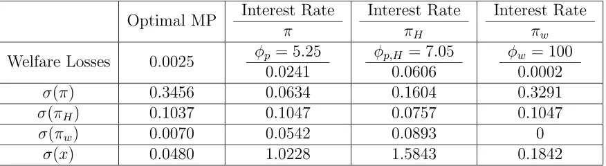
Table 1 reports the welfare losses associated with each interest rate rule12. Under the
baseline calibration the rule performing best is the one targeting wage inflation. But,
what is more important, domestic inflation targeting delivers welfare losses
consider-ably higher then CPI inflation targeting. The ability of a CPI inflation targeting rule
to outperform a domestic inflation targeting rule is particularly interesting given that
the volatility of CPI inflation does not enter into the loss function. The intuition for
this result is simple. As explained previously, because of sticky wages, fluctuations in
CPI inflation translate into undesired movements of the wage mark-up acting as an
endogenous cost push shock in the economy. Reducing the volatility of CPI inflation
reduces such cost push shock and therefore, reduces the trade off faced by the
mone-tary authority. For this reason, it makes it easier to stabilize wage inflation, domestic
inflation and output gap. Indeed, from table 1 it is clear that the rule targeting CPI
12The welfare losses are measured as percentage units of steady state consumption and are
inflation delivers much better results in terms of reducing the volatility of wage
in-flation and output gap than the rule targeting domestic inin-flation and this is why the
associated welfare losses are lower.
Therefore, the presence of wage rigidity rationalizes CPI inflation targeting in
contrast with the previous literature advocating for domestic inflation targeting.
Of course, those results have been derived under a baseline calibration. Even
though the calibration used is pretty standard, it is interesting to study how the
relative performance of the rules is affected by some crucial parameters. In the next
[image:33.612.109.547.394.514.2]section a comparison among the rules under different calibrations is presented.
Table 1.1: Welfare cost of deviation from optimal policy and standard de-viations associated to each policy rule.Welfare losses are in percentage units of steady state consumption. Standard deviations are also expressed in %. The coeffi-cients of the policy rule minimizing the welfare losses are also reported. A coefficient of 100 stands for strict inflation targeting.
Optimal MP Interest Rate
π
Interest Rate
πH
Interest Rate
πw
Welfare Losses 0.0025 φp = 5.25
0.0241
φp,H = 7.05
0.0606
φw = 100
0.0002
σ(π) 0.3456 0.0634 0.1604 0.3291
σ(πH) 0.1037 0.1047 0.0757 0.1047
σ(πw) 0.0070 0.0542 0.0893 0
σ(x) 0.0480 1.0228 1.5843 0.1842
1.6.3
Main robustness checks
The parameters over which a robustness check is performed are: the degree of wage
stickinessξw; the inverse of the labour supply elasticityϕ; the elasticity of substitution
between different types of labour θw; the elasticity of substitution between different
parameters is changed in each experiment while the others are kept at their baseline
calibration.
Wage stickiness The level of wage rigidity in the economy is probably the most
crucial parameter given that, as shown by Gal´ı and Monacelli (2005), when there is
no wage rigidity in the economy, the optimal monetary policy coincides with strict
domestic inflation targeting and a simple rule targeting domestic inflation outperforms
the one targeting CPI inflation. The first check is therefore to see which level of wage
rigidity is needed to invert this result.
0 0.1 0.2 0.3 0.4 0.5 0.6 0.7 0.8
−0.05 0 0.05 0.1 0.15 0.2 0.25 0.3
Comparinson among different MP rules for different degrees of wage rigidity
% welfare losses
Degree of wage rigidity in the economy
[image:34.612.113.536.270.607.2]CPI infl. targeting DI infl. targeting Wage infl. targeting
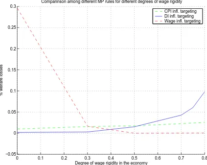
Figure 1.1: Wage Stickiness
From picture 1.1 we can notice that, while the performance of the rules targeting
in the economy, this is not the case for the rule targeting at CPI inflation. Indeed,
the wage inflation targeting rule performs really bad when there is no wage stickiness
and is overall the worst rule for levels of wage rigidity below 0.3 while it becomes the
best rule for levels of wage rigidity above 0.4. The opposite is true for the domestic
inflation targeting rule which coincides with the optimal monetary policy whenξw = 0
and is the best rule for low levels of wage rigidity. The threshold value for the two
price inflation targeting rules isξw = 0.5. Whenever the level of wage rigidity is above
such value, the rule targeting CPI inflation outperforms the one targeting domestic
inflation. Recall that the level of price rigidity under which the experiment is run is
the baseline value ξp = 0.75 i.e, the CPI inflation targeting rule has to be preferred
to the domestic inflation targeting rule even when the level of price rigidity in the
economy is higher then the degree of wage rigidity.
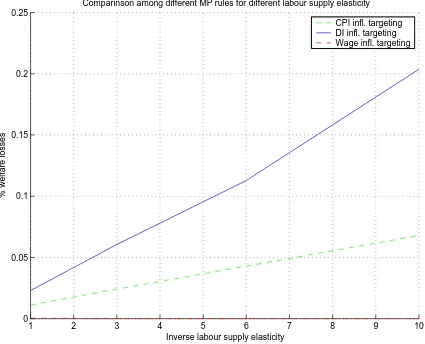
Labour supply elasticity An even more crucial parameter is the inverse of the
labour supply elasticity ϕ. Indeed, while it is very standard to assumeξw = 0.75, in
the literature different values forϕare used. The baseline calibration is 3. In figure 1.2 different welfare losses for values ofϕranging from 1 to 10 are reported. Independently on the level of labour supply elasticity, domestic inflation targeting is always worst
than CPI inflation targeting. Reducing the elasticity amplifies the distance between
the two rules. This is reasonable given that a lower elasticity (i.e a higherϕ) implies a bigger penalization of both output gap and wage inflation variability and we saw
under the baseline calibration that domestic inflation targeting fails to contain the
variability of those two variables.
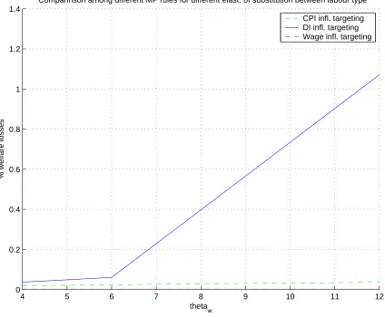
Wage markup Another parameter for which different calibrations can be found in
the literature is the elasticity of substitution between different labour types, θw. In
the baseline calibration it has been set to 6, implying a wage markup of 1.2. In figure
1 2 3 4 5 6 7 8 9 10 0
0.05 0.1 0.15 0.2 0.25
Comparinson among different MP rules for different labour supply elasticity
% welfare losses
Inverse labour supply elasticity
[image:36.612.113.538.77.421.2]CPI infl. targeting DI infl. targeting Wage infl. targeting
Figure 1.2: Inverse labour elasticity
parameter does not alter the ranking of the rules. However, for values of θw above 6
the performance of the domestic inflation targeting rule progressively worsen. This
is again due to the fact that a high elasticity of substitution implies a high weight on
the loss function to wage volatility.
1.6.4
Other checks
We have done other robustness checks for which the pictures are not reported for
brevity.
4 5 6 7 8 9 10 11 12 0
0.2 0.4 0.6 0.8 1 1.2 1.4
Comparinson among different MP rules for different elast. of substitution between labour type
% welfare losses
theta
w
[image:37.612.114.538.80.430.2]CPI infl. targeting DI infl. targeting Wage infl. targeting
Figure 1.3: Wage Mark-up
volatility in the loss function but, given that the rules all deliver very similar volatility
for this variable, changing this parameter does not change the results at all.
Decreasing the degree of price rigidity clearly worsen the performance of domestic
inflation targeting and the same happens if we increase the autocorrelation coefficient
for the technological process ρa.
1.7
Conclusions
The question addressed in the paper is whether the introduction of wage rigidities
many central banks that are targeting CPI inflation. As in the closed economy case,
once both price and wage rigidities are present, it is no longer possible to reach the
flexible price allocation because the central bank cannot simultaneously stabilize price
inflation, wage inflation and the output gap. Given this, an interesting question was
if it were still true that targeting domestic inflation is the best that a central bank can
do. To this purpose, we derived the loss function from a second order approximation of
the utility of the representative consumer. After deriving the optimal monetary policy
under commitment, we then simulated the model under different simple interest rate
rules, in order to make a ranking among them, using the optimal monetary policy as
a benchmark. The main result is that, under the baseline calibration a rule targeting
domestic inflation delivers considerably larger welfare losses than a rule targeting
CPI inflation. Several robustness checks have been provided, confirming all the same
results. Therefore we can conclude that wage stickiness provides a rational for CPI
Labor Market Institutions and
Inflation Volatility in the Euro
Area
1
2.1
Introduction
Inflation differentials are still pronounced among euro area countries despite the
ex-istence, for many years, of a common currency, a single market for products, capital
and labor (though with low labor mobility) and tightly harmonized fiscal policies.
Why is it so? Research to date has concentrated on differentials in inflation levels,
explaining their size and persistence on the basis of convergence mechanisms such as
the ”Balassa Samuelson”, or asymmetric national shocks (in aggregate demand, or
supply, or in the degree of exposure to area-wide external shocks), whose effect are
typically exacerbated by high inflation persistence2. Here we look instead at inflation
1
Joint with Ester Faia.
2
See European Central Bank Inflation report Eur (2003) for a non-technical survey and Hon-ohan and Lane (2003) and Angeloni and Ehrmann (2007), and the references therein, for some interpretations of the evidence.
volatility differentials and study their link with labor market institutions –
specif-ically, the replacement rate which is the ratio between unemployment benefit and
wage.
We think that the properties of euro area inflation we document and the
expla-nation we offer may be deeper and more long-lasting than those studied by other
authors. While convergence phenomena are by nature transient, and inflation
persis-tence in the eurozone can be expected to decline as a result of product market reforms
and enhanced central bank credibility, labor market structures (unemployment
insur-ance in particular) are deeply entrenched in national preferences3 and hence should
be expected to vary little over time. Linking them to inflation volatility differentials
hence means pointing at features of inflation asymmetry in the EMU that will be very
difficult to remove, even at much higher levels of economic and financial integration
than that prevailing at present.
Labor market characteristics influence the dynamics of real wages and of the
marginal cost of firms, which, in the standard New-Keynesian model, are a main
driver of inflation. Hence it seems natural to assess the quantitative relevance of
such institutions in determining differentials in inflation behavior. Specifically, the
intuition behind our reasoning is the following. Consider e.g. a shock that reduces
real wages in a given country in EMU. If the replacement rate is lower, workers face a
worse outside option and therefore are willing to accept a bigger reduction in wage in
order to keep their jobs. Assuming little or no labor mobility, in the country with low
replacement rate we should observe in equilibrium a higher reduction in real wage,
marginal costs as well as inflation, since inflation is linked to marginal costs via the
Phillips curve. In general, the volatility of real wages, marginal costs and inflation is
inversely related to the replacement rate. The shape of the relation depends not only
on labor market characteristics but on the whole shock and propagation mechanisms,
including (since EMU countries are highly integrated in trade and capital markets)
the cross-country spillovers.
Our analysis proceeds as follows. We first document the negative empirical
rela-tion between volatilities of de-trended real wages, marginal costs and inflarela-tion and
replacement rates4 during the EMU period. Secondly, we build a DSGE model with
two countries sharing the same currency, characterized by matching frictions and
wage rigidity in the labor market5, monopolistic competition and adjustment cost
on pricing. The two-country model accounts for the rich structure of propagation
mechanisms and international spillovers existing in a monetary union. We use this
laboratory economy, calibrated on the euro area, to analyze the effect of shocks under
different values of the replacement rates, and find that the model also gives rise to a
negative relation. Finally, we match the model results with the empirical ones, and
find that the model replicates well the relations found in the data.
In section 2.2 we present our empirical stylized facts; in section 2.3 we present
the model and its calibration, in section 2.4 we show the model results and we match
them with the data. Section 2.5 concludes.
2.2
Stylized Facts
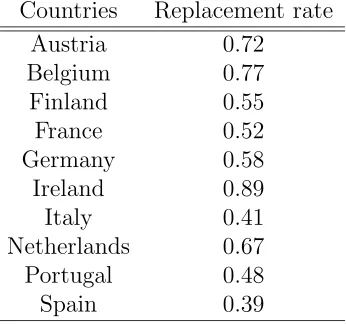
Table (2.1) shows averages over 1998 to 2004 of replacement rates for a series of euro
area countries. Data are taken from Nickell and Nunziata (2007). As a measure
of unemployment insurance coverage they use the benefit replacement rate (BBR,
benefit as a ratio to average earnings before taxes) provided by OECD, which is a
4As calculated by Nickell and Nunziata (2007).
5The tradition of introducing matching frictions in DSGE closed economy model is well
measure of the monetary loss incurred by the worker when moving from the employed
to the unemployed status. To proxy a dynamic concept of unemployment insurance
benefit, Nickell and Nunziata calculate a weighted average of the BRR over the first
5 years of unemployment; for example, the first entry in the table means that an
Austrian worker in the first 5 years of unemployment earns on average 89 percent of
her last wage when employed.
Several features of the data are worth noting. First, there is considerable
cross-country variation, from a minimum of 0.39 to a maximum of 0.89; this seems a large
enough span to have an observable macroeconomic impact. It is worth noticing that
we observe much cross-country variation but little time variation6, suggesting that
indeed the BRR incorporates deeply entrenched features of the national systems. In
the literature this parameter is often use as a catch-all measure of unemployment
insurance, and is assumed to be a key determinant in the worker’s decision to keep
a job. A further advantage of this measure is that it is easily comparable across
countries.
In our analysis we consider the euro area countries during the period
1998Q1-2004Q4. 1998 is included in the sample because during most of that year exchange
rates were virtually constant and EMU was expected with certainty to start at the
beginning of the following year (in fact, the ECB as created in mid-1998, not in
1999 as often assumed). Among the original EMU members, we exclude Luxembourg
because there are no data on replacement rates, hence making a total of 10 countries7.
In figure 2.1 (panels a, b and c) we plot on the vertical axis the volatilities of wage,
of unit labor costs and inflation, all measured relative to the volatility of output in
6Despite the fact that some countries have undertaken reforms in the last decade there is still a
considerable cross-country variation. In comparing replacement rates data across different periods (pre and post EMU) we came across two observations. First, all EMU countries have undertaken reforms that increased the size and duration of the unemployment benefits. Secondly, despite those reforms the relative ranking across countries remained the same as there was still little convergence.
the corresponding countries8, and on the horizontal axis the replacement rates9.
Inflation rates are measured by the GDP deflator. As measure of real wages we
use the hourly earnings divided by the CPI and as a measure of marginal cost the unit
labor cost. Data are taken from OECD. The standard deviations have been computed
on Hodrick-Prescott filtered series. In all three charts we drew two interpolating
lines, a linear and an exponential one. All lines shows a negative relation, and the
exponential is convex relative to the origin. The evidence of a negative and convex
relation seems quite clear and robust across the three measures of volatility. Overall
the relations are statistically significant apart from the one on marginal cost10.
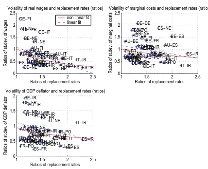
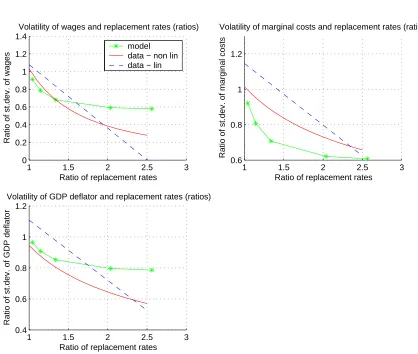
Figure 2.2 (panels a, b and c) shows the same variables, but this time as ratios
between pairs of countries11. Hence each dot shows, for a given pair of countries,
the ratio between the standard deviations (relative to that of output) of real wages,
marginal costs and inflation, respectively, plotted against the corresponding ratios of
the replacement rates. We show these transformations of the original data because
this is the appropriate way to match the model results with the data, as explained
below. The negative relation, linear and non-linear, is again clear and statistically
significant.
8We divided by the volatility of output to have a standardized measure.
9Replacement rates are averages over the period 1998-2004.
10It is a well known problem in the literature that measures of marginal costs are often associated
with low statistical significance. The reason for this is that marginal costs are approximated in the data by measures of average costs. Such an approximation is valid under the assumption of Cobb-Douglas production function. However this assumption might easily fail to hold.
2.3
A Model for A Currency Area with Labor
Mar-ket Frictions
There are two countries of equal size. Each economy is populated by households who
consume different varieties of domestically produced and imported goods, save and
work. Households save in both domestic and internationally traded bonds. Each
agent can be either employed or unemployed. In the first case he receives a wage
that is determined according to a Nash bargaining, in the second case he receives an
unemployment benefit. The labor market is characterized by matching frictions and
endogenous job separation. The production sector acts as a monopolistic competitive
sector which produces a differentiated good using capital and labor as inputs and
faces adjustment costs a’ la Rotemberg (1982).
2.3.1
Households in the Domestic and Foreign Country
Let’s denote12 by c
t ≡[(1−γ)
1
ηc η−1
η
h,t +γ
1 ηc η−1 η f,t ] η
η−1 a composite consumption index of
domestic and imported bundles of goods, where γ is the balanced-trade steady state share of imported goods (i.e., an inverse measure of home bias in consumption
prefer-ences), andη >0 is the elasticity of substitution between domestic and foreign goods. Optimal allocation of expenditure between domestic and foreign bundles yields:
ch,t = (1−γ)
ph,t
pt
−η
ct; cf,t=γ
pf,t
pt
−η
ct (2.1)
Each bundle is then composed of imperfectly substitutable varieties (with elasticity of
substitutionε >1).There is continuum of agents who maximize the expected lifetime utility.
12Let
st = {s
0, ....st} denote the history of events up to date t, where st denotes the event realization at datet. The date 0 probability of observing historystis given byρt. The initial state
s0 is given so that
ρ0 = 1. Henceforth, and for the sake of simplifying the notation, let’s define
the operatorEt{.} ≡Pst+1ρ(s
t+1|